easymodeller

USER MANUAL

EasyModeller 2.0

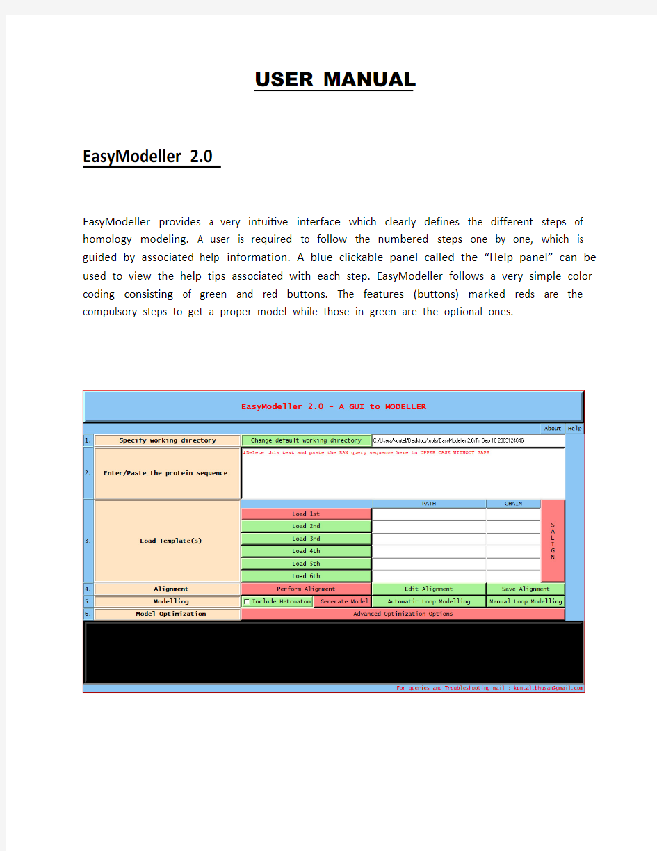
EasyModeller provides a very intuitive interface which clearly defines the different steps of homology modeling. A user is required to follow the numbered steps one by one, which is guided by associated help information. A blue clickable panel called the “Help panel” can be used to view the help tips associated with each step. EasyModeller follows a very simple color coding consisting of green and red buttons. The features (buttons) marked reds are the compulsory steps to get a proper model while those in green are the optional ones.

STEP 1: Specifying working directory

The first step involves specifying the working directory, which is the folder location where the output files will be generated. By default the working directory is created where the application is installed with a name of the current system date and time, and the path is displayed in the text box beside. The working directory location can be changed by editing the path displayed in the text box associated with “change default working directory” in step 1. The working directory if changed should be done at the start of a job and should not be changed in the middle. When starting a new job it is advisable to restart the application or make a new job name by editing the path in the text box otherwise the previous files will be overwritten and the previous job information might be lost.

STEP 2: Entering the query sequence

The second and most basic step is entering the amino acid sequence information as the input parameter. This query protein sequence to be modeled must be pasted or entered in the text window associated with step numbered 2 after deleting the help text displayed there in red font. The query sequence should be the raw sequence of the protein, i.e., should contain only the amino acid sequence in upper case without gaps and not in any other format like FASTA.

STEP 3: Loading template(s)

The third step is providing the template information to the program. The user should load a proper template structure(s) in standard formats like (.pdb, .ent, etc) which are acceptable to MODELLER by Load template(s) feature. For performing single template based homology modeling the “Load 1st” feature should be selected which allows the user to browse through and select the template file from the appropriate location. To do multi template based modeling which requires more than one template, a user should load all the template structure files one by one in order with a maximum of six templates. Immediately after loading a template the template path is displayed in the PATH text box and the first chain in the template is displayed in the CHAIN text box. Along with this the basic template information like the compound name, available chains and heteroatom information in extracted from the template and displayed in the display text box for user convenience. To include a different chain for modeling the user should manually edit and change the default chain id. The chain id should be left blank if no chain is found in the template loaded. After this, the SALIGN feature should be selected which performs a structure alignment of all the template structures using the salign() function of MODELLER. To maintain a consistency, even while performing single template based modeling the SALIGN feature should be selected.

STEP 4: Alignment

The next step of homology modeling is aligning the query sequence with the temple which is achieved in step four. The “Perform Alignment” feature aligns the query sequence with the template(s) using the align2d() function of MODELLER and displays the output alignment in the text display window of the tool. Although align2d() is based on a dynamic programming algorithm, it is different from standard sequence-sequence alignment methods because it takes into account structural information from the template when constructing an alignment. This task is achieved through a variable gap penalty function that tends to place gaps in solvent exposed and curved regions, outside secondary structure segments, and between two positions that are close in space. As a result, the alignment errors are reduced by approximately one third relative to those that occur with standard sequence alignment techniques. This improvement becomes more important as the similarity between the sequences decreases and the number of gaps increases. A very useful feature of the tool is the possibility to view and manually improve the query alignment via the feature ‘Edit Alignment’. The user can modify the default alignment that appears in the display text field or paste a new alignment but necessarily in the same format which appears after selecting the “Edit Alignment” feature and then save it by selecting “Save Alignment”. The default alignment displayed in the display text field after selecting the “Perform Alignment” feature shows the indexed ( _aln.pos ) query template alignment with the conserved residues ( _consrvd ) marked as star symbol (*) along with the secondary structure information in the standard MODELLER convention, i.e. average content of helical residues for structures at each position, 0 for 0% and 9 for 100% ( _helix ) and average content of beta-strand residues for structures at each position, 0 for 0% and 9 for 100%.( _beta ) as shown in Fig. 2. Along with this the standard MODELLER output is also displayed in the accompanied verbose screen which gives advanced information about the alignment. Based on this information the user can keep the alignment or modify it to get a better model. External alignment editing applications like Bioedit can be used to manually edit the “.ali” files in the working directory.

STEP 5: Model generation

The fifth step is generating the homology model by using the information generated so far. The “Generate Model” feature is used to achieve this by using the appropriate MODELLER function as required. Three possible options exist to get a model single template based, multi template based and single template with heteroatom. In all the cases the automodel class of MODELLER is used. To get a model by including the heteroatom the user should select the “Include Heteroatom” checkbox and then select “Generate Model”. On completion of model generation the generated model is displayed in the default PDB viewer installed in the system and a successful completion message is displayed in the display text window as well as in the verbose

output which displays the standard MODELLER model quality parameters (molpdf, DOPE score and GA341 score) along with. To keep the process simple only one model, which is the best as per MODELLER quality parameters is generated.

STEP 6: Loop modeling

Further the generated model can be improved upon by loop modeling. MODELLER has several loop optimization methods, which all rely on scoring functions and optimization protocols adapted for loop modeling. They are used to refine loop regions, either automatically after standard model building, or manually on an existing PDB file. EasyModeller can be used for both. In many cases, a better quality loops can be obtained (at the expense of more computer time) by using the DOPE-based loop modeling protocol. This can be done by automatic loop modeling which is achieved in the tool by selecting the option by the same name. On the other hand the manual loop modeling feature can be used to refine the conformation of the loop between a specified the starting and ending residue. Upon selecting the “Manual loop modeling” option a query window is displayed which allows the user to load a structure, specify the starting and ending residue number and selecting the “Run” option to perform the task. For all loop modeling the loopmodel class of MODELLER is used.

STEP 7: Model optimization

The final step is model optimization which when selected displays a new window titled advanced optimization options. The window allows the query model to be optimized to be loaded into the program.

Following this the “Optimize model” option can be selected to optimize the model which calls the optimizers module in MODELLER. The “optimizers module” provides a number of methods to optimize a model. The molecular pdf is optimized with respect to the selected coordinates, and the optimized coordinates are returned. These optimizers are often used to implement the variable target function method, for example in the automodel and loopmodel classes. Calling the object's optimize method then performs a number of optimizing iterations using a modified version of the Beale restart conjugate gradients method. Further a very basic molecular dynamics can be performed on the loaded model which uses the same module and implements the Verlet algorithm. The various parameters for optimization and dynamics like temperature and number of iterations can be changed by editing the default value in the corresponding text boxes. The minimized models are generated for every 10 steps and are saved in the working directory inside a new folder optimized models. The dynamics output binary trajectory files are also saved in the same folder which can be read in by visualization software such as CHIMERA

or VMD. Further the model profile plot can be generated by selecting the “Plot profile of a model” option which calculates DOPE energy of the loaded model using the assess_dope() function. Since EasyModeller uses the Microsoft Excel plot function to plot the profile graph, it is necessary to have Microsoft Excel installed in the system. It should be remembered that these scores are not absolute, so we cannot make a direct numerical comparison between two models based on the DOPE score. However, we can get an idea of the quality of our input alignment this way by comparing the rough shapes of the two profiles - if one is obviously shifted relative to the other, it is likely that the alignment is also shifted from the correct one.