Multi-frame image restoration for face recognition

MULTI-FRAME IMAGE RESTORATION FOR FACE RECOGNITION Frederick W.Wheeler,Xiaoming Liu,Peter H.Tu and Ralph T.Hoctor

Visualization and Computer Vision Lab

GE Global Research,Niskayuna,NY,USA

{wheeler,liux,tu,hoctor}@https://www.360docs.net/doc/03624513.html,

ABSTRACT

Face recognition at a distance is a challenging and important law-enforcement surveillance problem,with low image reso-lution and blur contributing to the dif?culties.We present a method for combining a sequence of video frames of a sub-ject in order to create a restored image of the face with re-duced blur.A generic Active Appearance Model of face shape and appearance is used for registration.By warping and av-eraging registered video frames,noise is reduced,allowing a Wiener?lter to deblur the face to a greater degree than can be achieved on a single video frame.This process is theoret-ically justi?ed and tested with real-world outdoor video us-ing a PTZ camera and a commercial face recognition engine. Improvement is demonstrated for both face recognition and authentication.

1.INTRODUCTION

Automatic face recognition at a distance is of growing impor-tance to many real-world law enforcement surveillance appli-cations.However,performance of existing face recognition systems is often inadequate due to the low-resolution of sub-ject probe images[1].Our present goal is to improve the accu-racy and extend the range of face recognition through multi-frame facial image restoration from video.

In surveillance systems,a subject is typically captured on video.Current commercial face recognition algorithms work on still images so face recognition applications generally ex-tract a single frame with a suitable view of the face.In a sense,this is throwing away a great deal of information.We expect to improve facial image resolution and face recogni-tion by exploiting the fact that the face is seen in many video frames,and combining those frames to make a single restored facial image.

The?eld of image super-resolution is concerned with us-ing multiple images or video frames of the same object or scene to make one image of superior quality[2,3,4].Quality This project was supported by award#2005-IJ-CX-K060awarded by the National Institute of Justice,Of?ce of Justice Programs,US Department of Justice.The opinions,?ndings,and conclusions or recommendations ex-pressed in this publication are those of the authors and do not necessarily re?ect the views of the Department of Justice.improvement can come from noise reduction through averag-ing,deblurring,and de-aliasing.It is also possible to improve image quality through modeling,or use of a statistical prior, though such methods are equally applicable and bene?cial to single image restoration[5].It is generally accepted that super-resolution is achieved when the restored image contains information above the Nyquist frequency of the individual ob-served images,and this can be achieved with signal process-ing.

In principle the faces can be super-resolved given accu-rate registration and an PSF that passes spatial frequencies above the Nyquist frequency.As an intermediate step in our progress in this area we demonstrate here improved facial res-olution and sharpness gained through registration,noise re-duction and classic Wiener image restoration.Our current baseline multi-frame restoration approach is described in this paper.Given video of an unknown subject we?t an Active Appearance Model(AAM)[6,7]to the face in each frame.A set of about10consecutive frames are then combined to pro-duce the restored image.A base frame of reference at twice the pixel resolution and the same orientation as the central video frame is de?ned.Each video frame is warped using bilinear interpolation to the base frame using the registration de?ned by the AAM.These warped frames are averaged and deblurred using a Wiener?lter[8,9].While this is techni-cally not super-resolution in the sense de?ned above,signi?-cant image deblurring is achieved and this baseline approach shows clear improvement in image quality.

To validate the bene?t of this technique we utilize the commercial face recognition package FaceIt R SDK ver.6.1 (Identix Inc.)with single video frames and restored images. Our goal is to determine the degree to which face recognition and veri?cation is improved by the image restoration process. Tests are performed using video collected in real-world out-door conditions in our surveillance testbed.

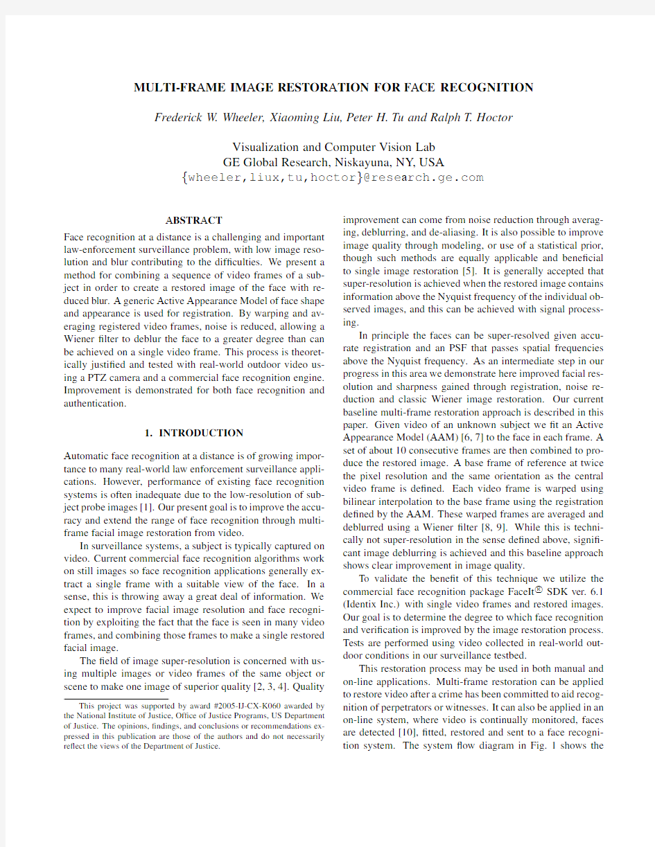
This restoration process may be used in both manual and on-line applications.Multi-frame restoration can be applied to restore video after a crime has been committed to aid recog-nition of perpetrators or witnesses.It can also be applied in an on-line system,where video is continually monitored,faces are detected[10],?tted,restored and sent to a face recogni-tion system.The system?ow diagram in Fig.1shows the

Fig.1.Major components of a complete face recognition system using multi-frame restoration.

major components of an enhanced face recognition system making use of multi-frame restoration.

2.ACTIVE APPEARANCE MODEL

This section provides an overview of the relatively complex process of training and?tting an Active Appearance Model (AAM)for faces.For this image restoration application the AAM provides the frame-to-frame registration of the face area of each video frame.

The?rst step in multi-frame restoration is registration.In order to combine the frames,for a pair of frames we must know the mapping,x2=f(x1),that converts the?rst im-age coordinates,x1=(r1,c1),of a real object or scene point to the second image coordinates,x2=(r2,c2).In most ap-plications,registration is heavily constrained.Typically the registration is parameterized as simple shifts in the X and Y direction,or as an af?ne transform or homography[11]. However,the registration may also be extremely general,such as with optical image?ow[12].In general it is best to se-lect a parameterized registration function that can accurately model the actual frame-to-frame motion,with no additional freedom.With this in mind we use an Active Appearance Model for face registration.

An AAM applied to faces is a two-stage model of both facial shape and appearance designed to?t the faces of dif-ferent persons at different orientations.The model has two parts,a shape model and an appearance model.The shape model describes the distribution of the2D or3D locations of a set of landmark points.Figure2(a)shows the33feature points used here.The shape model is trained using a large set of images from the Notre Dame Biometrics database Col-lection D[13,14]on which the feature point locations were found manually.Instead of allowing the feature points to be distributed arbitrarily,Principle Components Analysis(PCA) and the training data are used to reduce the dimensionality of the face shape space while capturing the major modes of variation across the training set population.

The AAM shape model includes a mean face shape that is the average of all face shapes in the training set and a set of eigenvectors.The mean face shape is the canonical shape and is used as the frame of reference for the AAM appear-ance model.Each training set image is warped to the canon-ical shape frame of reference.Now,all faces are presented as if they had the same shape.With shape variation now re-moved,the variation in appearance of the faces is modeled in this second stage,again using PCA to select a set of appear-ance eigenvectors for dimensionality reduction.

The complete trained AAM can produce face images that continually vary over appearance and shape.For our pur-poses,the AAM is used to lock on to a new face as it ap-pears in a video frame.This is accomplished by solving for the face shape and appearance parameters(eigenvector coef-?cients)such that the model-generated face matches the face in the video frame using the Simultaneous Inverse Composi-tional(SIC)algorithm[7].While both shape parameters and appearance parameters need to be estimated to?t the model to a new face in a frame,only the resulting shape parameters are used for registration.

While this section gives a brief overview of the general application of an AAM to facial images,the AAM used in this work[15]has two signi?cant additional features.It is multi-resolution so the AAM native resolution is more appropriate for the video frame resolution.Also,the model is iteratively re?ned during training,signi?cantly reducing?tting time and making?tting more robust to initialization.Figure3shows an example of AAM?tting results for video frames.

The AAM provides the registration needed to align the face across the video frames.The AAM is?t to the face in each video frame.The shape model portion of the AAM then de?nes33landmark positions in each frame.These landmark positions are the vertices of a set49triangles over the face as seen in Fig.2(a).The registration of the face region be-tween any two frames is a piecewise af?ne transformation, with an af?ne transformation in each triangle de?ned by the corresponding triangle vertices.

3.WIENER FILTERING

In this section we provide a basic overview of Wiener?ltering and how the multi-frame restoration method will increase the level of deblurring achieved by a Wiener?lter.

Our model for video frames is that a perfect continuous image of the scene is convolved with a Point Spread Function

(a)(b)(c)

Fig.2.(a)Face from video with 33AAM landmarks;(b)additional border landmarks;(c)blending

mask.

Fig.3.Faces from 8consecutive video frames and the ?tted AAM shape model.

(PSF),sampled on an image grid,corrupted by additive white Gaussian noise,and quantized.The PSF is responsible for the blur and it is our desire to reduce this blur.The additive noise will be the limiting factor in our ability to do this.As is typically done,we assume that the dominant source of noise is CCD electronic noise,and that the noise is i.i.d.additive Gaussian,and thus has a ?at spectrum.With all image signals represented in the spatial frequency domain,if the transform of the original image is I (ω1,ω2),the Optical Transfer Func-tion (OTF,the Fourier Transform of the PSF)is H (ω1,ω2)

and the additive Gaussian noise signal is ?N

(ω1,ω2),then the observed video frame is,

G (ω1,ω2)=H (ω1,ω2)I (ω1,ω2)+?N

(ω1,ω2)(1)

The Wiener ?lter is a classic method for single image de-blurring [8,9],providing the Minimum Mean Squared Error (MMSE)estimate of I (ω1,ω2),the non-blurred image given a noisy blurred observation,G (ω1,ω2).With no assumption made about the unknown image signal,the Wiener ?lter is,

?I

(ω1,ω2)=H ?(ω1,ω2)

|H (ω1,ω2)|2+K

G (ω1,ω2)

(2)

where H ?(ω1,ω2)is the complex conjugate of H (ω1,ω2).If parameter K is the noise to signal power ratio then we have

the MMSE Wiener ?lter.In practice K is adjusted to balance

noise ampli?cation and sharpening.If K is too large the im-age will not have high spatial frequencies restored to the full extent possible.If K is too small the restored image will be corrupted by ampli?ed high spatial frequency noise.As K goes to zero,and assuming H (ω1,ω2)>0,the Wiener ?lter approaches the ideal inverse ?lter,

?I

(ω1,ω2)=1

H (ω1,ω2)

G (ω1,ω2)

(3)

The inverse ?lter greatly ampli?es high-frequency noise and is generally not a well conditioned operation.

The effect of the Wiener ?lter on a blurred noisy image is to pass spatial frequencies that are not attenuated by the PSF and have a high SNR;to amplify spatial frequencies that are attenuated by the PSF and have a high SNR;and to attenuate spatial frequencies that have a low SNR.This is seen in 1-D in Fig.4for the case of a Gaussian shaped PSF and several val-ues for K .In Fig.4(a)is the spatial domain PSF with σ=2.For a Gaussian shaped PSF,the OTF is Gaussian shaped as well,shown in Fig.4(b)with the frequency variable ωnor-malized so that with spatial domain sampling at the integers,the Nyquist frequency is 0.5.The ideal inverse of the OTF in Fig.4(c)would amplify high-frequency noise an extreme

(a)(b)(c)(d)(e)

Fig.4.(a)spatial domain Gaussian PSF(h(x));(b)corresponding frequency domain OTF(H(ω));(c)unrealizable inverse of OTF(1/H(ω));(d)Wiener?lter for K=0.5,0.2,0.1,0.05(H?(ω)/(|H(ω)|2+K));(e)total response for each Wiener?lter (|H(ω)|2/(|H(ω)|2+K)).

amount.Figure4(d)shows the Wiener?lter for several val-ues of K.Notice how when K is reduced(less image noise) the higher spatial frequencies are more ampli?ed.Figure4(e) shows the product of the OTF and the Wiener?lter.This rep-resents the total system response.As K is reduced higher spatial frequencies are more strongly restored by the Wiener ?lter.For suf?ciently low K,the total response passband in Fig.4(e)is wider than the OTF in Fig.4(b)so the restored im-age will have greater apparent resolution and sharpness than the observed image.

This example shows how reducing image noise allows a Wiener?lter to restore high-spatial frequencies to a greater degree,improving resolution and sharpness.In the following section,the multi-frame method for reducing image noise is described.

4.MULTI-FRAME RESTORATION

Our baseline multi-frame restoration algorithm works by av-eraging the aligned face region of N consecutive video frames and applying a Wiener?lter[8,9]to the result.The frame averaging reduces additive image noise and the Wiener?l-ter deblurs the effect of the PSF.The Wiener?lter applied to the time averaged frame is able to reproduce the image at high spatial frequencies that were attenuated by the PSF more accurately than a Wiener?lter applied to a single video frame.Reproducing the high spatial frequencies more accu-rately means the restored image will have higher effective res-olution and more detail.The reason is that the image noise at these high spatial frequencies was reduced through the av-eraging process.Just as averaging N independent measure-ments of a value,each measurement corrupted by zero-mean additive Gaussian noise with varianceσ2gives an estimate of that value that has a variance ofσ2/N,averaging N regis-tered and warped images reduces the additive noise variance, and the appropriate value of K by a factor of1/N.

The AAM provides registration only for the portion of the face within the triangles.If only this region is used,the regis-tered frame mean will have a border that is at the edge of the face.This sharp discontinuity will result in strong rippling edge effects after deblurring.To mitigate this we extrapolate the registration by adding to the set of face landmarks to de-?ne an extended border region.The30new landmarks are simply positioned some?xed distance out from the estimated face edges,and form45new triangles at the border,seen in Fig.2(b).Registration will not be accurate in this border re-gion,however,we have found it to be suf?cient to eliminate restoration?lter artifacts caused by the discontinuity.

For the set of N video frames,a new base frame of refer-ence is created by selecting the middle video frame and dou-bling its pixel resolution.Each video frame is then warped to the base frame of reference.The registration function is piecewise af?ne,and bilinear interpolation is used.This aligns the face in each video frame.The aligned faces frames are then averaged to make a mean frame.

To deblur,a Wiener?lter is applied to the aligned face mean frame.For most installed surveillance cameras it is dif-?cult to determine the true PSF,so we assume a Gaussian shaped PSF with hand selected width,σ,and image noise to signal power ratio,K.For an on-line or repeatedly used sys-tem this would need to be done only once.Frame averaging allows reduction of parameter K by a factor of1/N and thus further ampli?cation of high spatial frequencies.Wiener?l-tering is performed in the frequency domain using the FFT. All other operations,registration,warping,and averaging,are performed in the spatial domain.

A sample restoration result appears in Fig.5.This?g-ure shows(a)the face from an original video frame,(b)that single frame restored with a Wiener?lter with K=0.1(the best result found by hand),(c)the result of multi-frame en-hancement using N=8consecutive frames using low-noise assumption K=0.01(the best result found by hand)and(d) the same single frame restored using the incorrect low-noise assumption K=0.01.With multi-frame enhancement,we restore higher spatial frequencies because K is lower in(c). When that same low value for K is used to attempt to restore high spatial frequencies in a single frame in(d),the result is poor and shows signi?cant artifacts because the single frame has more noise.The restored image in(c)is sharper and more detailed than the original frame and the Wiener?ltered origi-

(a)(b)(c)(d)

Fig.5.(a)Original video frame;(b)Wiener ?ltered single video frame (K =0.1);(c)Multi-frame restoration result (K =0.01);(d)Wiener ?ltered single video frame incorrectly using the same value of K as was used for the multi-frame restoration result (K =0.01).nal frame.

5.BLENDING

Outside of the face region modeled by the AAM,frame-to-frame registration is not determined.The multi-frame restora-tion technique improves the quality of the face region,but not the other regions of the image.To make a more pleasing ?nal

result,the restored face image,?I

,is blended with a ?ll image,I f .The ?ll image is the single middle unrestored video frame upsampled to match the pixel resolution of the restored image.The ?ll image is the source of the base frame of reference so it lines up perfectly with the restored face image.

A mask M is de?ned in the base frame that has value 1inside the face region and fades to zero outside of that region linearly with distance to the face region.This mask is used to blend the restored image with the ?ll image,I f using,

I (r,c )=M (r,c )?I

(r,c )+(1?M (r,c ))I f (r,c )(4)

Figure 2(c)shows an example of the mask image.The result in Fig.5(c)has been blended using this procedure.

The result after blending is an image with improved fa-cial resolution and a background that is at the original frame resolution,but is not distracting to a viewer and appears more natural to automatic face recognition algorithms.

6.EXPERIMENTAL RESULTS AND CONCLUSIONS To validate the restoration algorithm we have collected out-door video of 3test subjects using a GE CyberDome R

PTZ camera.The PTZ camera was zoomed at intervals to cap-ture video at different face resolutions,measured as eye dis-tance in pixels.A 700person gallery was created with 3good quality images of the test subjects and the “FA”image of the ?rst 697subjects in the FERET database [16].From

FAR (%)

F R R (%)

Fig.7.ROC performance for authentication with a watch-list improved with enhancement.Arrows indicate performance improvement due to multi-frame restoration.

the test video sequences we extracted original frames and cre-ated multi-frame restored facial images from the surrounding set of N =10frames.Figure 6shows the rank 1–5recog-nition counts and rates for the original frames and enhanced images.The results are grouped by face resolution and also combined.We see a noticeable trend of improvement,espe-cially for small original face resolutions.Even this straight-forward multi-frame restoration process bene?ts recognition under these dif?cult conditions.

The original and enhanced face images were also tested in veri?cation mode against the 700person gallery used as a watch-list.Figure 7shows the False Recognition Rate (FRR)vs.False Alarm Rate (FAR)operational performance for eye distances of 37and 29pixels in the original video,where we

Eye Dist.483729241917all Num.Probes243624182115138 Enhanced no yes no yes no yes no yes no yes no yes no yes Rank-116182626161581145147179 Rank-2192027281616101156157886 Rank-3202027301718111266158291 Rank-4202127321819111276258595 Rank-5212128331819121278368999 Rank-167%75%72%72%67%63%44%61%19%24%7%27%51%57% Rank-279%83%75%78%67%67%56%61%24%29%7%33%57%62% Rank-383%83%75%83%71%75%61%67%29%29%7%33%59%66% Rank-483%88%75%89%75%79%61%67%33%29%13%33%62%69% Rank-588%88%78%92%75%79%67%67%33%38%20%40%64%72% Fig.6.Rank recognition counts and rate(%),with and without multi-frame restoration,grouped by eye distance(pixels)in the original video frames.

saw the most signi?cant improvement.

As we develop methods for face recognition from video by combining and preprocessing multiple-frames we present our initial baseline algorithm and encouraging results on dif-?cult real-world face video.

7.REFERENCES

[1]D.M.Blackburn,J.M.Bone,and P.J.Phillips,FRVT

2000Evaluation Report,February2001.

[2]Subhasis Chaudhuri,Ed.,Super-Resolution Imaging,

Kluwer Academic Publishers,3rd edition,2001.

[3]K.J.Ray Liu,Moon Gi Kang,and Subhasis Chaudhuri,

Eds.,IEEE Signal Processing Magazine,Special edi-tion:Super-Resolution Image Reconstruction,vol.20, no.3,IEEE,May2003.

[4]Sean Borman and Robert Stevenson,“Super resolu-

tion enhancement of low-resolution image sequences;

a comprehensive review with directions for future re-

search,”Research report,University of Notre Dame, July1998.

[5]Simon Baker and Takeo Kanade,“Limits on super-

resolution and how to break them,”IEEE Transactions on Pattern Analysis and Machine Intelligence,vol.24, no.9,pp.1167–1183,September2002.

[6]T.Cootes,D.Cooper,C.Tylor,and J.Graham,“A

trainable method of parametric shape description,”in Proc.2nd British Machine Vision Conference.Septem-ber1991,pp.54–61,Springer.

[7]S.Baker and I.Matthews,“Lucas-Kanade20years on:

A unifying framework,”International Journal of Com-

puter Vision,vol.56,no.3,pp.221–255,March2004.

[8]Anil K.Jain,Fundamentals of Digital Image Process-

ing,Prentice Hall,1989.

[9]Rafael C.Gonzalez and Paul Wintz,Digital Image Pro-

cessing,Addison-Wesley Publishing Co.,2nd edition, 1987.

[10]H.Schneiderman,“Learning a restricted bayesian net-

work for object detection,”in Proceedings of the IEEE Conference on Computer Vision and Pattern Recogni-tion,2004.

[11]Richard Hartley and Andrew Zisserman,Multiple View

Geometry in Computer Vision,Cambridge University Press,2000.

[12]Simon Baker and Takeo Kanade,“Super resolution op-

tical?ow,”Tech.Rep.CMU-RI-TR-99-36,Robotics In-stitute,Carnegie Mellon University,Pittsburgh,PA,Oc-tober1999.

[13]K.Chang,K.W.Bowyer,and P.J.Flynn,“Face recogni-

tion using2D and3D facial data,”in ACM Workshop on Multimodal User Authentication,December2003,pp.

25–32.

[14]P.J.Flynn,K.W.Bowyer,and P.J.Phillips,“Assess-

ment of time dependency in face recognition:An initial study,”in Audio and Video-Based Biometric Person Au-thentication,2003,pp.44–51.

[15]Xiaoming Liu,Peter Tu,and Frederick Wheeler,“Face

model?tting on low resolution images,”in submitted to British Machine Vision Conference,2006.

[16]P.J.Phillips,H.Moon,P.J.Rauss,and S.Rizvi,“The

FERET evaluation methodology for face recognition al-gorithms,”IEEE Transactions on Pattern Analysis and Machine Intelligence,vol.22,no.10,October2000.