AMESIM
15th International Congress on Sound and Vibration
6-10 July 2008, Daejeon, Korea
MODELING AND SIMULATION STUDIES OF 1-DOF HYDRAULIC SERVO VIBRATION PLATFORM BASED ON
AMESIM
Zhiqiang Chao, Renwei Diao, Aihong Meng, Shousong Han and Pengcheng Jiang
Department of Mechanical Engineering, the Academy of Armored Force Engineering
Beijing 100072, China
Email: fengfuzhou@https://www.360docs.net/doc/0a6271269.html, or feng_maxj@https://www.360docs.net/doc/0a6271269.html,
Abstract
In this paper, 1-DOF hydraulic servo vibration platform is designed, and its mathematical models are constructed; Based on the control theory, a repetitive control method is proposed to improve the tracking accuracy of the system’s periodic response. Through the interface between Simulink and AMESim, co-simulation is achieved, and the validity of the method is verified.
1. INTRODUCTION
The actual road test which costs more and is not proper for repeating experiment is restricted by geographic and weather conditions. With the development of modern control theory, and computer technology, the bench scale test becomes more and more important in the auto industry. Through this kind of simulation we can get many results such as fatigue life, durability, vibration characteristics of the vehicle’s structure, driver’s comfort and so on. In addition, the vibration platform can provide all necessary vibration conditions, which is more intuitive and effective to observe and analyze the reliability of the body and suspension system, as well as the causation of the fatigue damage. In this paper, 1-DOF hydraulic servo vibration platform is designed, and its mathematical models are constructed. A repetitive control method is proposed to improve the tracking accuracy of the system’s periodic response, and simulation is performed based on “Advanced Modeling Environment for Simulation (AMESim)”and MATLAB.
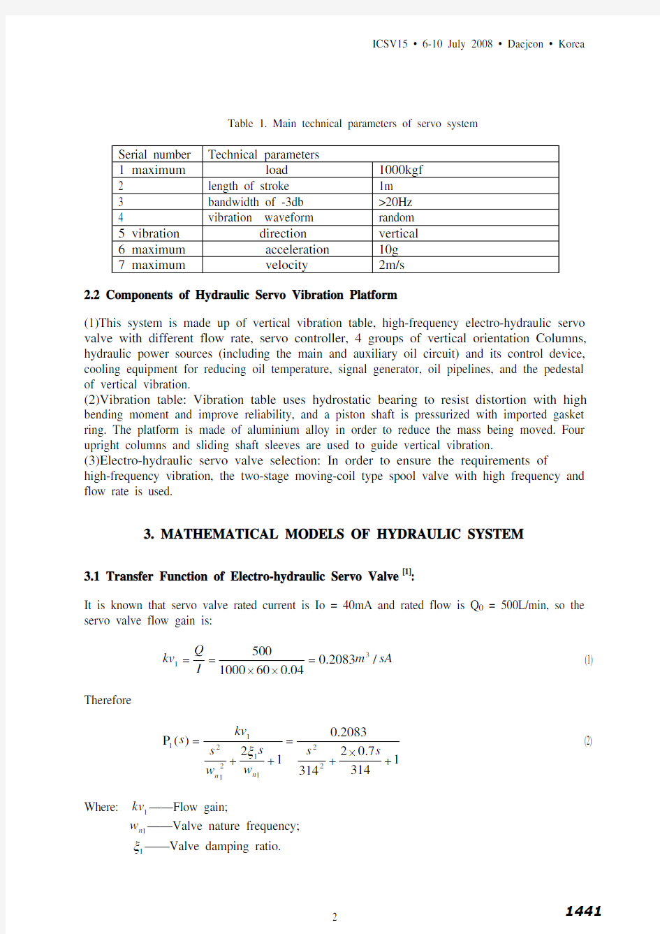
2. PARAMETERS OF VIBRATION PLATFORM AND ITS COMPONENTS 2.1 Main Technical Parameters of Servo System
Table 1. Main technical parameters of servo system
Serial number Technical parameters
1 maximum load 1000kgf
2 length of stroke 1m
3 bandwidth of -3db >20Hz
4 vibration waveform random
5 vibration direction vertical
6 maximum acceleration 10g
7 maximum velocity 2m/s
2.2 Components of Hydraulic Servo Vibration Platform
(1)This system is made up of vertical vibration table, high-frequency electro-hydraulic servo valve with different flow rate, servo controller, 4 groups of vertical orientation Columns, hydraulic power sources (including the main and auxiliary oil circuit) and its control device, cooling equipment for reducing oil temperature, signal generator, oil pipelines, and the pedestal of vertical vibration.
(2)Vibration table: Vibration table uses hydrostatic bearing to resist distortion with high bending moment and improve reliability, and a piston shaft is pressurized with imported gasket ring. The platform is made of aluminium alloy in order to reduce the mass being moved. Four upright columns and sliding shaft sleeves are used to guide vertical vibration.
(3)Electro-hydraulic servo valve selection: In order to ensure the requirements of high-frequency vibration, the two-stage moving-coil type spool valve with high frequency and flow rate is used.
3. MATHEMATICAL MODELS OF HYDRAULIC SYSTEM
3.1 Transfer Function of Electro-hydraulic Servo Valve [1]:
It is known that servo valve rated current is Io = 40mA and rated flow is Q 0 = 500L/min, so the servo valve flow gain is:
sA m I Q kv /2083.004
.060100050031=××== (1)
Therefore
13147.023142083.012)(P 221121
211+×+=++=s s w s w s kv s n n ξ (2)
Where: ——Flow gain;
1kv ——Valve nature frequency;
1n w 1ξ——Valve damping ratio.
3.2 Transfer Function of Actuating Unit [1]:
12782.022789.19812/1)(P 22222
222+×+=++=s s s s A s n n ωξω (3)
Where: A——Area of piston;
2n ω——Nature frequency of the actuating unit;
2ξ——Damping ratio of actuating unit.
3.3 Open-loop Transfer Functions of Hydraulic System [1]:
)12782.02278
)(13147.20314(43.41)(P 2222+×+++=s s s s s s (4)
4. THE AMESIM/MATLAB CO-SIMULATION
4.1 Software Introduction
AMESim has a graphical modeling environment with great amount of engineering packages which are used to design system, such as hydraulic simulation package which contains lots of hydraulic components, hydraulic resources, and hydraulic pipes, etc. The models of these components consider the compressibility of hydraulic oil, and the nonlinear characteristics of components (hysteresis effect, dead band, leaking, static friction, dynamic friction, and damping ratio, etc). This software has a powerful post-processing feature, which provides a good support for engineering analysis. The following are key features: (1) comprising rich model libraries; (2) using C or FORTRAN to program and due to its open code, users can build their individual components; (3) more advanced users can also use Export and AMEPilot to co-simulate with other software such as MATLAB and ADAMS [2].
In this paper, firstly AMESim is used to construct a subsystem model for the parts of the mechanical and hydraulic. Secondly construct the AMESim model as an S-Function in order to achieve the joint with MATLAB/Simulink. Thirdly complete the control system in Simulink. At last, AMESim and Simulink will run simultaneously so that you can use the full facilities of both packages.
4.2 Modeling and Simulation
The AMESim model is shown in Figure 1, and the followings are the parameters of system components [3]:
Servo valve: rated flow 500L/min, natural frequency 50Hz, damping ratio 0.7, dead band 0.1%, zero-leakage 1.2 ×mm/min, valve rated current 40mA.
Cylinder: total mass being moved 1000 kg, piston diameter 80mm, diameter of rod 45mm, length of stroke 1m, viscous friction coefficient 20000N/(m/s).
310?
Hydraulic accumulator: gas pressure 17MPa, gas precharge pressure 25MPa, accumulator volume 32L.
Pump: fixed displacement 100cc/min.
Motor: shaft speed 1450r/min.
Figure 1. The model of AMESim
Figure 2. The model of MATLAB
The control model is shown in Figure 2, and repetitive control is used to reduce deviation. Under the repetitive control, the last deviation is added on the present one to control objects. After the study in the initial periods, the input signal can be tracked accurately [4]. If the period of signal r (t) is L, and the following conditions are met,
①is canonical;
[](s)K (s) P (s) C I + ②is in gradual stability;
-1s)]C(s)P(s)K([I +③1]C(s)P(s)s)]C(s)P(s)K(I [I 2
-1<+?, where “I” stands for identity matrix, the repetitive control system will be in a stable state, and the deviation will be converged. Therefore, when C(s) is equalled to the transfer function of conventional PID, the repetitive control system will be stable; K(s) is to improve system stability and the rapidity. We often choose ; F(s) generally is defined as low-pass filter, and 1 K(s)=1)(≈ωj F c Ω∈?ω, where c c ωωω<=Ω: stands for the tracking range [5].
The control algorithm [6] is as follows:
R(s)Y(s) E(s)=
s)C(s)P(s)U(Y(s)=
W(s)V(s)U(s)+=
)()(1)()(21s E e
s F e s F s V Ls Ls
???= K(s)E(s)W(s)=
If we choose , the deviation of closed-loop system is:
1 K(s)=
[][][]
Ls Ls Ls
e
s F e s F s P s C e s F s R s E ????++?=)()(1)()(1)(1)()(212 (5) Provided 1)(≈ωj F , obviously the deviation is reduced. When the sine signal r=0.5+0.3sin(t) is imported, the simulation results for repetitive control are shown in Figure 3, and deviation response is shown in Figure 4. It is clear that repetitive control can track the imported signal. In the steady state, the largest deviation is e=0.03m which is 10% of the imported signal, but in common PID control the largest deviation is 30%. Comparing Figure 3 and Figure 4 with Figure 5 and Figure 6, the tracking precision of repetitive control has improved a lot.
The curve of flow rate and pressure of cylinder is shown in Figure 7 and 8. We could see from the curves that the pulsation of flow rate and pressure is small. We can conclude that the system runs in a steady state.