多模态论文

A DAM :A M ETHOD FOR S TOCHASTIC O PTIMIZATION

Diederik P.Kingma *

University of Amsterdam,OpenAI

dpkingma@https://www.360docs.net/doc/0a12851463.html,

Jimmy Lei Ba ?University of Toronto

jimmy@psi.utoronto.ca

A BSTRACT

We introduce Adam ,an algorithm for ?rst-order gradient-based optimization of stochastic objective functions,based on adaptive estimates of lower-order mo-ments.The method is straightforward to implement,is computationally ef?cient,has little memory requirements,is invariant to diagonal rescaling of the gradients,and is well suited for problems that are large in terms of data and/or parameters.The method is also appropriate for non-stationary objectives and problems with very noisy and/or sparse gradients.The hyper-parameters have intuitive interpre-tations and typically require little tuning.Some connections to related algorithms,on which Adam was inspired,are discussed.We also analyze the theoretical con-vergence properties of the algorithm and provide a regret bound on the conver-gence rate that is comparable to the best known results under the online convex optimization framework.Empirical results demonstrate that Adam works well in practice and compares favorably to other stochastic optimization methods.Finally,we discuss AdaMax ,a variant of Adam based on the in?nity norm.

1I NTRODUCTION

Stochastic gradient-based optimization is of core practical importance in many ?elds of science and engineering.Many problems in these ?elds can be cast as the optimization of some scalar parameter-ized objective function requiring maximization or minimization with respect to its parameters.If the function is differentiable w.r.t.its parameters,gradient descent is a relatively ef?cient optimization method,since the computation of ?rst-order partial derivatives w.r.t.all the parameters is of the same computational complexity as just evaluating the function.Often,objective functions are stochastic.For example,many objective functions are composed of a sum of subfunctions evaluated at different subsamples of data;in this case optimization can be made more ef?cient by taking gradient steps w.r.t.individual subfunctions,i.e.stochastic gradient descent (SGD)or ascent.SGD proved itself as an ef?cient and effective optimization method that was central in many machine learning success stories,such as recent advances in deep learning (Deng et al.,2013;Krizhevsky et al.,2012;Hinton &Salakhutdinov,2006;Hinton et al.,2012a;Graves et al.,2013).Objectives may also have other sources of noise than data subsampling,such as dropout (Hinton et al.,2012b)regularization.For all such noisy objectives,ef?cient stochastic optimization techniques are required.The focus of this paper is on the optimization of stochastic objectives with high-dimensional parameters spaces.In these cases,higher-order optimization methods are ill-suited,and discussion in this paper will be restricted to ?rst-order methods.

We propose Adam ,a method for ef?cient stochastic optimization that only requires ?rst-order gra-dients with little memory requirement.The method computes individual adaptive learning rates for different parameters from estimates of ?rst and second moments of the gradients;the name Adam is derived from adaptive moment estimation.Our method is designed to combine the advantages of two recently popular methods:AdaGrad (Duchi et al.,2011),which works well with sparse gra-dients,and RMSProp (Tieleman &Hinton,2012),which works well in on-line and non-stationary settings;important connections to these and other stochastic optimization methods are clari?ed in section 5.Some of Adam’s advantages are that the magnitudes of parameter updates are invariant to rescaling of the gradient,its stepsizes are approximately bounded by the stepsize hyperparameter,it does not require a stationary objective,it works with sparse gradients,and it naturally performs a form of step size annealing.

?

Equal contribution.Author ordering determined by coin ?ip over a Google Hangout.

a r X i v :1412.6980v 9 [c s .L G ] 30 J a n 2017

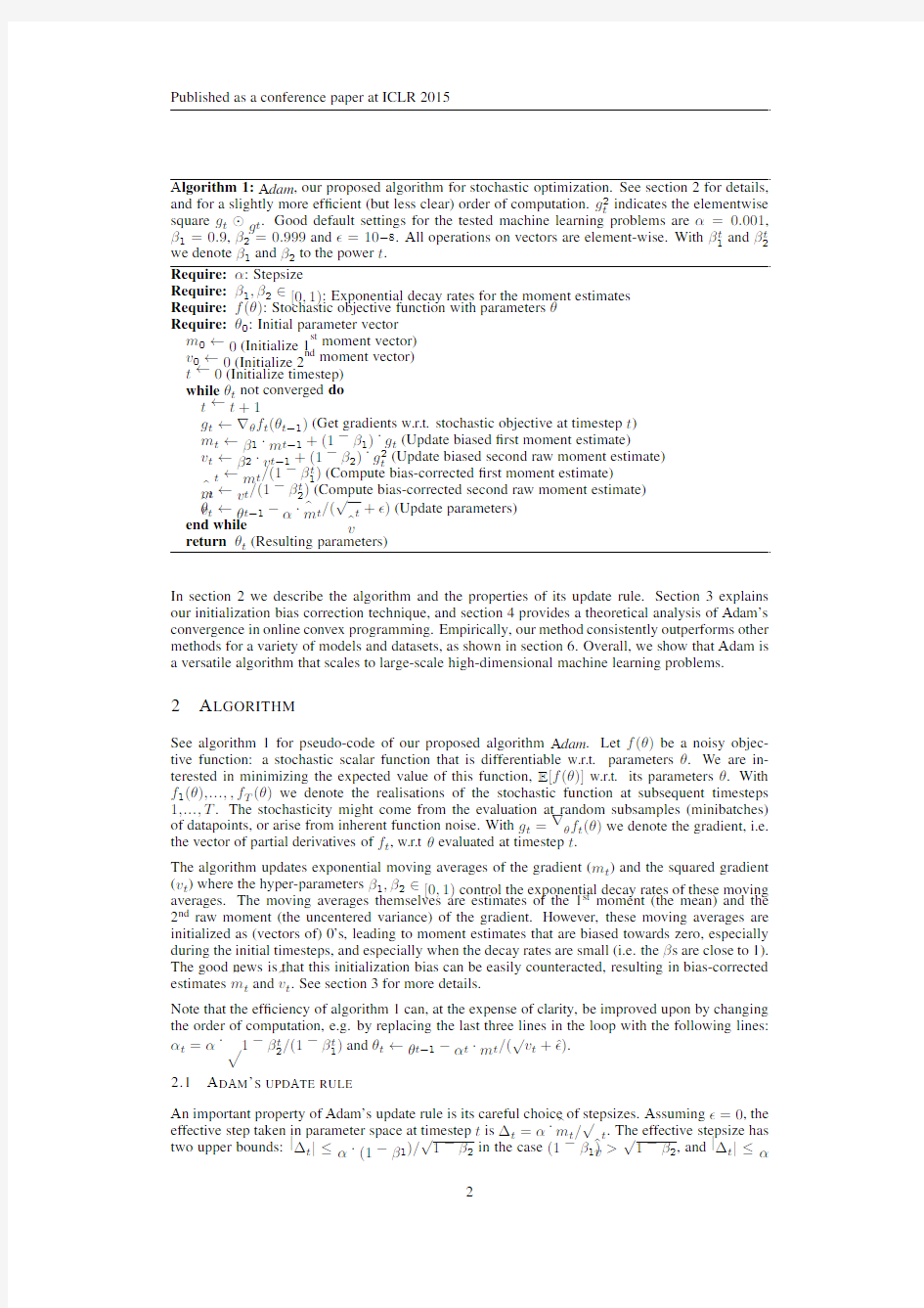
Algorithm 1:Adam ,our proposed algorithm for stochastic optimization.See section 2for details,

and for a slightly more ef?cient (but less clear)order of computation.g 2

t indicates the elementwise square g t g t .Good default settings for the tested machine learning problems are α=0.001,

β1=0.9,β2=0.999and =10?8.All operations on vectors are element-wise.With βt 1and βt

2we denote β1and β2to the power t .Require:α:Stepsize

Require:β1,β2∈[0,1):Exponential decay rates for the moment estimates Require:f (θ):Stochastic objective function with parameters θRequire:θ0:Initial parameter vector m 0←0(Initialize 1st moment vector)v 0←0(Initialize 2nd moment vector)t ←0(Initialize timestep)while θt not converged do t ←t +1

g t ←?θf t (θt ?1)(Get gradients w.r.t.stochastic objective at timestep t )m t ←β1·m t ?1+(1?β1)·g t (Update biased ?rst moment estimate)

v t ←β2·v t ?1+(1?β2)·g 2

t (Update biased second raw moment estimate)

m t ←m t /(1?βt

1)(Compute bias-corrected ?rst moment estimate)

v t ←v t /(1?βt

2)(Compute bias-corrected second raw moment estimate)θt ←θt ?1?α· m t /(√ v t + )(Update parameters)end while

return θt (Resulting parameters)In section 2we describe the algorithm and the properties of its update rule.Section 3explains our initialization bias correction technique,and section 4provides a theoretical analysis of Adam’s convergence in online convex programming.Empirically,our method consistently outperforms other methods for a variety of models and datasets,as shown in section 6.Overall,we show that Adam is a versatile algorithm that scales to large-scale high-dimensional machine learning problems.

2A LGORITHM

See algorithm 1for pseudo-code of our proposed algorithm Adam .Let f (θ)be a noisy objec-tive function:a stochastic scalar function that is differentiable w.r.t.parameters θ.We are in-terested in minimizing the expected value of this function,E [f (θ)]w.r.t.its parameters θ.With f 1(θ),...,,f T (θ)we denote the realisations of the stochastic function at subsequent timesteps 1,...,T .The stochasticity might come from the evaluation at random subsamples (minibatches)of datapoints,or arise from inherent function noise.With g t =?θf t (θ)we denote the gradient,i.e.the vector of partial derivatives of f t ,w.r.t θevaluated at timestep t .

The algorithm updates exponential moving averages of the gradient (m t )and the squared gradient (v t )where the hyper-parameters β1,β2∈[0,1)control the exponential decay rates of these moving averages.The moving averages themselves are estimates of the 1st moment (the mean)and the 2nd raw moment (the uncentered variance)of the gradient.However,these moving averages are initialized as (vectors of)0’s,leading to moment estimates that are biased towards zero,especially during the initial timesteps,and especially when the decay rates are small (i.e.the βs are close to 1).The good news is that this initialization bias can be easily counteracted,resulting in bias-corrected estimates m t and v t .See section 3for more details.Note that the ef?ciency of algorithm 1can,at the expense of clarity,be improved upon by changing the order of computation,e.g.by replacing the last three lines in the loop with the following lines:

αt =α· t 2/(1?βt 1)and θt ←θt ?1?αt ·m t /(√v t +? ).2.1

A DAM ’S UPDATE RULE

An important property of Adam’s update rule is its careful choice of stepsizes.Assuming =0,the

effective step taken in parameter space at timestep t is ?t =α· m t /√ v t .The effective stepsize has two upper bounds:|?t |≤α·(1?β1)/√1?β2in the case (1?β1)>√1?β2,and |?t |≤α

otherwise.The ?rst case only happens in the most severe case of sparsity:when a gradient has been zero at all timesteps except at the current timestep.For less sparse cases,the effective stepsize will be smaller.When (1?β1)=√1?β2we have that | m t /√ v t |<1therefore |?t |<α.In more common scenarios,we will have that m t /√ v t ≈±1since |E [g ]/ E [g 2]|≤1.The effective magnitude of the steps taken in parameter space at each timestep are approximately bounded by the stepsize setting α,i.e.,|?t | α.This can be understood as establishing a trust region around the current parameter value,beyond which the current gradient estimate does not provide suf?cient information.This typically makes it relatively easy to know the right scale of αin advance.For many machine learning models,for instance,we often know in advance that good optima are with high probability within some set region in parameter space;it is not uncommon,for example,to have a prior distribution over the parameters.Since αsets (an upper bound of)the magnitude of steps in parameter space,we can often deduce the right order of magnitude of αsuch that optima can be reached from θ0within some number of iterations.With a slight abuse of terminology,we will call the ratio m t /√ v t the signal-to-noise ratio (SNR ).With a smaller SNR the effective stepsize ?t will be closer to zero.This is a desirable property,since a smaller SNR means that there is greater uncertainty about whether the direction of m t corresponds to the direction of the true gradient.For example,the SNR value typically becomes closer to 0towards an optimum,leading to smaller effective steps in parameter space:a form of automatic annealing.The effective stepsize ?t is also invariant to the scale of the gradients;rescaling the gradients g with factor c will scale m t with a factor c and v t with a factor c 2,which cancel out:(c · m t )/(√c 2· v t )= m t /√ v t .

3I NITIALIZATION BIAS CORRECTION

As explained in section 2,Adam utilizes initialization bias correction terms.We will here derive the term for the second moment estimate;the derivation for the ?rst moment estimate is completely analogous.Let g be the gradient of the stochastic objective f ,and we wish to estimate its second raw moment (uncentered variance)using an exponential moving average of the squared gradient,with decay rate β2.Let g 1,...,g T be the gradients at subsequent timesteps,each a draw from an underlying gradient distribution g t ～p (g t ).Let us initialize the exponential moving average as v 0=0(a vector of zeros).First note that the update at timestep t of the exponential moving average

v t =β2·v t ?1+(1?β2)·g 2t (where g 2

t indicates the elementwise square g t g t )can be written as a function of the gradients at all previous timesteps:

v t =(1?β2)

t i =1

βt ?i 2·g 2i

(1)

We wish to know how E [v t ],the expected value of the exponential moving average at timestep t ,

relates to the true second moment E [g 2

t

],so we can correct for the discrepancy between the two.Taking expectations of the left-hand and right-hand sides of eq.(1):

E [v t ]=E (1?β2)t

i =1

βt ?i 2·g 2

i (2)

=E [g 2

t ]·(1?β2)t i =1

βt ?i

2+ζ

(3)=

E [g 2t ]

·(1?

βt

2)

+ζ

(4)

where ζ=0if the true second moment E [g 2

i ]is stationary;otherwise ζcan be kept small since the exponential decay rate β1can (and should)be chosen such that the exponential moving average

assigns small weights to gradients too far in the past.What is left is the term (1?βt

2)which is caused by initializing the running average with zeros.In algorithm 1we therefore divide by this term to correct the initialization bias.

In case of sparse gradients,for a reliable estimate of the second moment one needs to average over many gradients by chosing a small value of β2;however it is exactly this case of small β2where a lack of initialisation bias correction would lead to initial steps that are much larger.

4C ONVERGENCE ANALYSIS

We analyze the convergence of Adam using the online learning framework proposed in (Zinkevich,2003).Given an arbitrary,unknown sequence of convex cost functions f 1(θ),f 2(θ),...,f T (θ).At each time t ,our goal is to predict the parameter θt and evaluate it on a previously unknown cost function f t .Since the nature of the sequence is unknown in advance,we evaluate our algorithm using the regret,that is the sum of all the previous difference between the online prediction f t (θt )and the best ?xed point parameter f t (θ?)from a feasible set X for all the previous steps.Concretely,the regret is de?ned as:

R (T )=T

t =1

[f t (θt )?f t (θ?)]

(5)

where θ?=arg min θ∈X T

t =1f t (θ).We show Adam has O (√T )regret bound and a proof is given in the appendix.Our result is comparable to the best known bound for this general convex online learning problem.We also use some de?nitions simplify our notation,where g t ?f t (θt )and g t,i as the i th element.We de?ne g 1:t,i ∈R t as a vector that contains the i th dimension of the gradients over all iterations till t ,g 1:t,i =[g 1,i ,g 2,i ,···,g t,i ].Also,we de?ne γ

β21√β2

.Our following

theorem holds when the learning rate αt is decaying at a rate of t ?1

2and ?rst moment running average coef?cient β1,t decay exponentially with λ,that is typically close to 1,e.g.1?10?8.

Theorem 4.1.Assume that the function f t has bounded gradients, ?f t (θ) 2≤G , ?f t (θ) ∞≤G ∞for all θ∈R d and distance between any θt generated by Adam is bounded, θn ?θm 2≤D ,

θm ?θn ∞≤D ∞for any m,n ∈{1,...,T },and β1,β2∈[0,1)satisfy β21√β2

<1.Let αt =α

√

t and β1,t =β1λt ?1

,λ∈(0,1).Adam achieves the following guarantee,for all T ≥1.

R (T )≤D 22α(1?β1)d i =1 T v T,i +α(1+β1)G ∞(1?β1)√1?β2(1?γ)2d i =1

g 1:T,i 2+

d i =1D 2∞

G ∞√1?β22α(1?β1)(1?λ)2Our Theorem 4.1implies when the data features are sparse and bounded gradients,the sum-mation term can be much smaller than its upper bound d i =1 g 1:T,i 2<

T v T,i <

i =1 g 1:T,i 2]also apply to Adam.In particular,the adaptive method,such as Adam and Adagrad,can achieve O (log d √T ),an improvement over O (√

dT )for the non-adaptive method.Decaying β1,t towards zero is impor-tant in our theoretical analysis and also matches previous empirical ?ndings,e.g.(Sutskever et al.,2013)suggests reducing the momentum coef?cient in the end of training can improve convergence.Finally,we can show the average regret of Adam converges,

Corollary 4.2.Assume that the function f t has bounded gradients, ?f t (θ) 2≤G , ?f t (θ) ∞≤G ∞for all θ∈R d and distance between any θt generated by Adam is bounded, θn ?θm 2≤D , θm ?θn ∞≤D ∞for any m,n ∈{1,...,T }.Adam achieves the following guarantee,for all T ≥1.

R (T )

T =O (1√T

)This result can be obtained by using Theorem 4.1and d

i =1

g 1:T,i 2≤dG ∞√T .Thus,lim T →∞R (T )

T =0.

5R ELATED WORK

Optimization methods bearing a direct relation to Adam are RMSProp (Tieleman &Hinton,2012;Graves,2013)and AdaGrad (Duchi et al.,2011);these relationships are discussed below.Other stochastic optimization methods include vSGD (Schaul et al.,2012),AdaDelta (Zeiler,2012)and the natural Newton method from Roux &Fitzgibbon (2010),all setting stepsizes by estimating curvature

from ?rst-order information.The Sum-of-Functions Optimizer (SFO)(Sohl-Dickstein et al.,2014)is a quasi-Newton method based on minibatches,but (unlike Adam)has memory requirements linear in the number of minibatch partitions of a dataset,which is often infeasible on memory-constrained systems such as a GPU.Like natural gradient descent (NGD)(Amari,1998),Adam employs a preconditioner that adapts to the geometry of the data,since v t is an approximation to the diagonal of the Fisher information matrix (Pascanu &Bengio,2013);however,Adam’s preconditioner (like AdaGrad’s)is more conservative in its adaption than vanilla NGD by preconditioning with the square root of the inverse of the diagonal Fisher information matrix approximation.

RMSProp:An optimization method closely related to Adam is RMSProp (Tieleman &Hinton,2012).A version with momentum has sometimes been used (Graves,2013).There are a few impor-tant differences between RMSProp with momentum and Adam:RMSProp with momentum gener-ates its parameter updates using a momentum on the rescaled gradient,whereas Adam updates are directly estimated using a running average of ?rst and second moment of the gradient.RMSProp also lacks a bias-correction term;this matters most in case of a value of β2close to 1(required in case of sparse gradients),since in that case not correcting the bias leads to very large stepsizes and often divergence,as we also empirically demonstrate in section 6.4.

AdaGrad:An algorithm that works well for sparse gradients is AdaGrad (Duchi et al.,2011).Its

basic version updates parameters as θt +1=θt ?α·g t / t i =1g 2t .Note that if we choose β2to be in?nitesimally close to 1from below,then lim β2→1 v t =t ?1· t

i =1g 2

t .AdaGrad corresponds to a version of Adam with β1=0,in?nitesimal (1?β2)and a replacement of αby an annealed version αt =α·t ?1/2,namely θt ?α·t ?1/2· m t / lim β2→1 v t =θt ?α·t ?1/2·g t / t ?1· t

i =1g 2t

=θt ?α·g t /

t i =1g 2t .Note that this direct correspondence between Adam and Adagrad does

not hold when removing the bias-correction terms;without bias correction,like in RMSProp,a β2in?nitesimally close to 1would lead to in?nitely large bias,and in?nitely large parameter updates.

6E XPERIMENTS

To empirically evaluate the proposed method,we investigated different popular machine learning models,including logistic regression,multilayer fully connected neural networks and deep convolu-tional neural https://www.360docs.net/doc/0a12851463.html,ing large models and datasets,we demonstrate Adam can ef?ciently solve practical deep learning problems.

We use the same parameter initialization when comparing different optimization algorithms.The hyper-parameters,such as learning rate and momentum,are searched over a dense grid and the results are reported using the best hyper-parameter setting.6.1

E XPERIMENT :L OGISTIC R EGRESSION

We evaluate our proposed method on L2-regularized multi-class logistic regression using the MNIST dataset.Logistic regression has a well-studied convex objective,making it suitable for comparison of different optimizers without worrying about local minimum issues.The stepsize αin our logistic

regression experiments is adjusted by 1/√t decay,namely αt =α

√

t

that matches with our theorat-ical prediction from section 4.The logistic regression classi?es the class label directly on the 784dimension image vectors.We compare Adam to accelerated SGD with Nesterov momentum and Adagrad using minibatch size of 128.According to Figure 1,we found that the Adam yields similar convergence as SGD with momentum and both converge faster than Adagrad.

As discussed in (Duchi et al.,2011),Adagrad can ef?ciently deal with sparse features and gradi-ents as one of its main theoretical results whereas SGD is low at learning rare features.Adam with 1/√t decay on its stepsize should theoratically match the performance of Adagrad.We examine the sparse feature problem using IMDB movie review dataset from (Maas et al.,2011).We pre-process the IMDB movie reviews into bag-of-words (BoW)feature vectors including the ?rst 10,000most frequent words.The 10,000dimension BoW feature vector for each review is highly sparse.As sug-gested in (Wang &Manning,2013),50%dropout noise can be applied to the BoW features during

Figure1:Logistic regression training negative log likelihood on MNIST images and IMDB movie reviews with10,000bag-of-words(BoW)feature vectors.

training to prevent over-?tting.In?gure1,Adagrad outperforms SGD with Nesterov momentum by a large margin both with and without dropout noise.Adam converges as fast as Adagrad.The empirical performance of Adam is consistent with our theoretical?ndings in sections2and4.Sim-ilar to Adagrad,Adam can take advantage of sparse features and obtain faster convergence rate than normal SGD with momentum.

6.2E XPERIMENT:M ULTI-LAYER N EURAL N ETWORKS

Multi-layer neural network are powerful models with non-convex objective functions.Although our convergence analysis does not apply to non-convex problems,we empirically found that Adam often outperforms other methods in such cases.In our experiments,we made model choices that are consistent with previous publications in the area;a neural network model with two fully connected hidden layers with1000hidden units each and ReLU activation are used for this experiment with minibatch size of128.

First,we study different optimizers using the standard deterministic cross-entropy objective func-tion with L2weight decay on the parameters to prevent over-?tting.The sum-of-functions(SFO) method(Sohl-Dickstein et al.,2014)is a recently proposed quasi-Newton method that works with minibatches of data and has shown good performance on optimization of multi-layer neural net-works.We used their implementation and compared with Adam to train such models.Figure2 shows that Adam makes faster progress in terms of both the number of iterations and wall-clock time.Due to the cost of updating curvature information,SFO is5-10x slower per iteration com-pared to Adam,and has a memory requirement that is linear in the number minibatches. Stochastic regularization methods,such as dropout,are an effective way to prevent over-?tting and often used in practice due to their simplicity.SFO assumes deterministic subfunctions,and indeed failed to converge on cost functions with stochastic regularization.We compare the effectiveness of Adam to other stochastic?rst order methods on multi-layer neural networks trained with dropout noise.Figure2shows our results;Adam shows better convergence than other methods.

6.3E XPERIMENT:C ONVOLUTIONAL N EURAL N ETWORKS

Convolutional neural networks(CNNs)with several layers of convolution,pooling and non-linear units have shown considerable success in computer vision tasks.Unlike most fully connected neural nets,weight sharing in CNNs results in vastly different gradients in different layers.A smaller learning rate for the convolution layers is often used in practice when applying SGD.We show the effectiveness of Adam in deep CNNs.Our CNN architecture has three alternating stages of5x5 convolution?lters and3x3max pooling with stride of2that are followed by a fully connected layer of1000recti?ed linear hidden units(ReLU’s).The input image are pre-processed by whitening,and

6

Figure 2:Training of multilayer neural networks on MNIST images.(a)Neural networks using dropout stochastic regularization.(b)Neural networks with deterministic cost function.We compare with the sum-of-functions (SFO)optimizer (Sohl-Dickstein et al.,2014)

Figure 3:Convolutional neural networks training cost.(left)Training cost for the ?rst three epochs.(right)Training cost over 45epochs.CIFAR-10with c64-c64-c128-1000architecture.

dropout noise is applied to the input layer and fully connected layer.The minibatch size is also set to 128similar to previous experiments.

Interestingly,although both Adam and Adagrad make rapid progress lowering the cost in the initial stage of the training,shown in Figure 3(left),Adam and SGD eventually converge considerably faster than Adagrad for CNNs shown in Figure 3(right).We notice the second moment estimate v t vanishes to zeros after a few epochs and is dominated by the in algorithm 1.The second moment estimate is therefore a poor approximation to the geometry of the cost function in CNNs comparing to fully connected network from Section 6.2.Whereas,reducing the minibatch variance through the ?rst moment is more important in CNNs and contributes to the speed-up.As a result,Adagrad converges much slower than others in this particular experiment.Though Adam shows marginal improvement over SGD with momentum,it adapts learning rate scale for different layers instead of hand picking manually as in SGD.

7

6.4E XPERIMENT :BIAS -CORRECTION TERM

We also empirically evaluate the effect of the bias correction terms explained in sections 2and 3.Discussed in section 5,removal of the bias correction terms results in a version of RMSProp (Tiele-man &Hinton,2012)with momentum.We vary the β1and β2when training a variational auto-encoder (V AE)with the same architecture as in (Kingma &Welling,2013)with a single hidden layer with 500hidden units with softplus nonlinearities and a 50-dimensional spherical Gaussian latent variable.We iterated over a broad range of hyper-parameter choices,i.e.β1∈[0,0.9]and β2∈[0.99,0.999,0.9999],and log 10(α)∈[?5,...,?1].Values of β2close to 1,required for robust-ness to sparse gradients,results in larger initialization bias;therefore we expect the bias correction term is important in such cases of slow decay,preventing an adverse effect on optimization.In Figure 4,values β2close to 1indeed lead to instabilities in training when no bias correction term was present,especially at ?rst few epochs of the training.The best results were achieved with small values of (1?β2)and bias correction;this was more apparent towards the end of optimization when gradients tends to become sparser as hidden units specialize to speci?c patterns.In summary,Adam performed equal or better than RMSProp,regardless of hyper-parameter setting.

7

E XTENSIONS

7.1

A DA M AX

In Adam,the update rule for individual weights is to scale their gradients inversely proportional to a (scaled)L 2norm of their individual current and past gradients.We can generalize the L 2norm based update rule to a L p norm based update rule.Such variants become numerically unstable for large p .However,in the special case where we let p →∞,a surprisingly simple and stable algorithm emerges;see algorithm 2.We’ll now derive the algorithm.Let,in case of the L p norm,the stepsize

at time t be inversely proportional to v 1/p

t ,where:

v t =βp 2v t ?1+(1?βp

2)|g t |p

(6)=(1?

βp

2)

t i =1

βp (t ?i )

2

·|g i |p

(7)

Algorithm 2:AdaMax ,a variant of Adam based on the in?nity norm.See section 7.1for details.Good default settings for the tested machine learning problems are α=0.002,β1=0.9and

β2=0.999.With βt 1we denote β1to the power t .Here,(α/(1?βt

1))is the learning rate with the bias-correction term for the ?rst moment.All operations on vectors are element-wise.Require:α:Stepsize

Require:β1,β2∈[0,1):Exponential decay rates

Require:f (θ):Stochastic objective function with parameters θRequire:θ0:Initial parameter vector m 0←0(Initialize 1st moment vector)

u 0←0(Initialize the exponentially weighted in?nity norm)t ←0(Initialize timestep)while θt not converged do t ←t +1

g t ←?θf t (θt ?1)(Get gradients w.r.t.stochastic objective at timestep t )m t ←β1·m t ?1+(1?β1)·g t (Update biased ?rst moment estimate)

u t ←max(β2·u t ?1,|g t |)(Update the exponentially weighted in?nity norm)

θt ←θt ?1?(α/(1?βt

1))·m t /u t (Update parameters)end while

return θt (Resulting parameters)

Note that the decay term is here equivalently parameterised as βp

2instead of β2.Now let p →∞,

and de?ne u t =lim p →∞(v t )1/p

,then:

u t =lim p →∞

(v t )1/p =lim p →∞

(1?βp

2)t i =1

βp (t ?i )2·|g i |p 1/p

(8)

=lim p →∞

(1?βp 2)1/p

t

i =1

βp (t ?i )

2

·|g i |p

1/p

(9)

=lim

p →∞

t

i =1

β(t ?i )2·|g i |

p

1/p

(10)=max

βt ?12|g 1|,βt ?2

2|g 2|,...,β2|g t ?1|,|g t |

(11)

Which corresponds to the remarkably simple recursive formula:

u t =max(β2·u t ?1,|g t |)

(12)

with initial value u 0=0.Note that,conveniently enough,we don’t need to correct for initialization bias in this case.Also note that the magnitude of parameter updates has a simpler bound with AdaMax than Adam,namely:|?t |≤α.7.2

T EMPORAL AVERAGING

Since the last iterate is noisy due to stochastic approximation,better generalization performance is often achieved by averaging.Previously in Moulines &Bach (2011),Polyak-Ruppert averaging (Polyak &Juditsky,1992;Ruppert,1988)has been shown to improve the convergence of standard

SGD,where ˉθt =1t n k =1θk .Alternatively,an exponential moving average over the parameters can

be used,giving higher weight to more recent parameter values.This can be trivially implemented

by adding one line to the inner loop of algorithms 1and 2:ˉθt ←β2·ˉθt ?1+(1?β2)θt ,with ˉθ0=0.Initalization bias can again be corrected by the estimator θt =ˉθt /(1?βt 2

).8C ONCLUSION

We have introduced a simple and computationally ef?cient algorithm for gradient-based optimiza-tion of stochastic objective functions.Our method is aimed towards machine learning problems with

large datasets and/or high-dimensional parameter spaces.The method combines the advantages of two recently popular optimization methods:the ability of AdaGrad to deal with sparse gradients, and the ability of RMSProp to deal with non-stationary objectives.The method is straightforward to implement and requires little memory.The experiments con?rm the analysis on the rate of con-vergence in convex problems.Overall,we found Adam to be robust and well-suited to a wide range of non-convex optimization problems in the?eld machine learning.

9A CKNOWLEDGMENTS

This paper would probably not have existed without the support of Google Deepmind.We would like to give special thanks to Ivo Danihelka,and Tom Schaul for coining the name Adam.Thanks to Kai Fan from Duke University for spotting an error in the original AdaMax derivation.Experiments in this work were partly carried out on the Dutch national e-infrastructure with the support of SURF Foundation.Diederik Kingma is supported by the Google European Doctorate Fellowship in Deep Learning.

R EFERENCES

Amari,Shun-Ichi.Natural gradient works ef?ciently in learning.Neural computation,10(2):251–276,1998. Deng,Li,Li,Jinyu,Huang,Jui-Ting,Yao,Kaisheng,Yu,Dong,Seide,Frank,Seltzer,Michael,Zweig,Geoff, He,Xiaodong,Williams,Jason,et al.Recent advances in deep learning for speech research at microsoft. ICASSP2013,2013.

Duchi,John,Hazan,Elad,and Singer,Yoram.Adaptive subgradient methods for online learning and stochastic optimization.The Journal of Machine Learning Research,12:2121–2159,2011.

Graves,Alex.Generating sequences with recurrent neural networks.arXiv preprint arXiv:1308.0850,2013. Graves,Alex,Mohamed,Abdel-rahman,and Hinton,Geoffrey.Speech recognition with deep recurrent neural networks.In Acoustics,Speech and Signal Processing(ICASSP),2013IEEE International Conference on, pp.6645–6649.IEEE,2013.

Hinton,G.E.and Salakhutdinov,R.R.Reducing the dimensionality of data with neural networks.Science,313 (5786):504–507,2006.

Hinton,Geoffrey,Deng,Li,Yu,Dong,Dahl,George E,Mohamed,Abdel-rahman,Jaitly,Navdeep,Senior, Andrew,Vanhoucke,Vincent,Nguyen,Patrick,Sainath,Tara N,et al.Deep neural networks for acoustic modeling in speech recognition:The shared views of four research groups.Signal Processing Magazine, IEEE,29(6):82–97,2012a.

Hinton,Geoffrey E,Srivastava,Nitish,Krizhevsky,Alex,Sutskever,Ilya,and Salakhutdinov,Ruslan R.Im-proving neural networks by preventing co-adaptation of feature detectors.arXiv preprint arXiv:1207.0580, 2012b.

Kingma,Diederik P and Welling,Max.Auto-Encoding Variational Bayes.In The2nd International Conference on Learning Representations(ICLR),2013.

Krizhevsky,Alex,Sutskever,Ilya,and Hinton,Geoffrey E.Imagenet classi?cation with deep convolutional neural networks.In Advances in neural information processing systems,pp.1097–1105,2012.

Maas,Andrew L,Daly,Raymond E,Pham,Peter T,Huang,Dan,Ng,Andrew Y,and Potts,Christopher. Learning word vectors for sentiment analysis.In Proceedings of the49th Annual Meeting of the Association for Computational Linguistics:Human Language Technologies-Volume1,pp.142–150.Association for Computational Linguistics,2011.

Moulines,Eric and Bach,Francis R.Non-asymptotic analysis of stochastic approximation algorithms for machine learning.In Advances in Neural Information Processing Systems,pp.451–459,2011. Pascanu,Razvan and Bengio,Yoshua.Revisiting natural gradient for deep networks.arXiv preprint arXiv:1301.3584,2013.

Polyak,Boris T and Juditsky,Anatoli B.Acceleration of stochastic approximation by averaging.SIAM Journal on Control and Optimization,30(4):838–855,1992.

Roux,Nicolas L and Fitzgibbon,Andrew W.A fast natural newton method.In Proceedings of the27th International Conference on Machine Learning(ICML-10),pp.623–630,2010.

Ruppert,David.Ef?cient estimations from a slowly convergent robbins-monro process.Technical report, Cornell University Operations Research and Industrial Engineering,1988.

Schaul,Tom,Zhang,Sixin,and LeCun,Yann.No more pesky learning rates.arXiv preprint arXiv:1206.1106, 2012.

Sohl-Dickstein,Jascha,Poole,Ben,and Ganguli,Surya.Fast large-scale optimization by unifying stochas-tic gradient and quasi-newton methods.In Proceedings of the31st International Conference on Machine Learning(ICML-14),pp.604–612,2014.

Sutskever,Ilya,Martens,James,Dahl,George,and Hinton,Geoffrey.On the importance of initialization and momentum in deep learning.In Proceedings of the30th International Conference on Machine Learning (ICML-13),pp.1139–1147,2013.

Tieleman,T.and Hinton,G.Lecture6.5-RMSProp,COURSERA:Neural Networks for Machine Learning. Technical report,2012.

Wang,Sida and Manning,Christopher.Fast dropout training.In Proceedings of the30th International Confer-ence on Machine Learning(ICML-13),pp.118–126,2013.

Zeiler,Matthew D.Adadelta:An adaptive learning rate method.arXiv preprint arXiv:1212.5701,2012. Zinkevich,Martin.Online convex programming and generalized in?nitesimal gradient ascent.2003.

10

A PPENDIX

10.1

C ONVERGENCE P ROOF

De?nition 10.1.A function f :R d →R is convex if for all x ,y ∈R d ,for all λ∈[0,1],

λf (x )+(1?λ)f (y )≥f (λx +(1?λ)y )

Also,notice that a convex function can be lower bounded by a hyperplane at its tangent.Lemma 10.2.If a function f :R d →R is convex,then for all x ,y ∈R d ,

f (y )≥f (x )+?f (x )T (y ?x )

The above lemma can be used to upper bound the regret and our proof for the main theorem is constructed by substituting the hyperplane with the Adam update rules.

The following two lemmas are used to support our main theorem.We also use some de?nitions sim-plify our notation,where g t ?f t (θt )and g t,i as the i th element.We de?ne g 1:t,i ∈R t as a vector that contains the i th dimension of the gradients over all iterations till t ,g 1:t,i =[g 1,i ,g 2,i ,···,g t,i ]Lemma 10.3.Let g t =?f t (θt )and g 1:t be de?ned as above and bounded, g t 2≤G , g t ∞≤G ∞.Then,T t =1

g 2t,i

t ≤2G ∞ g 1:T,i 2Proof.We will prove the inequality using induction over T.

The base case for T =1,we have

g 21,i

≤2G ∞ g 1,i 2.For the inductive step,

T t =1

g 2t,i

t

=

T ?1 t =1

g 2t,i

t

+

g 2T,i

T

≤2G ∞ g 1:T ?1,i 2+

g 2T,i

T

=2G ∞

g 1:T,i 22?g 2T +

g 2T,i

T

From, g 1:T,i 22?g 2

T,i +g 4T,i

4 g 1:T,i 22

≥ g 1:T,i 22?g 2

T,i ,we can take square root of both side and

have,

g 1:T,i 22?g 2T,i

≤ g 1:T,i 2?

g 2

T,i

2 g 1:T,i 2≤ g 1:T,i 2?g 2T,i

2

T G 2∞

Rearrange the inequality and substitute the

g 1:T,i 22?g 2T,i term,

G ∞ g 1:T,i 22?g 2T +

g 2T,i

T

≤2G ∞ g 1:T,i

2

Lemma 10.4.Let γ β2

1

√β2

.For β1,β2∈[0,1)that satisfy β21√β2

<1and bounded g t , g t 2≤G ,

g t ∞≤G ∞,the following inequality holds

T t =1

m 2t,i t v t,i ≤21?γ1√1?β2 g 1:T,i 2

Proof.Under the assumption,√

1?βt

2(1?βt 1)2≤1

(1?β1)2.We can expand the last term in the summation using the update rules in Algorithm 1,

T t =1 m 2t,i t v t,i =T ?1 t =1

m 2t,i t v t,i

+ 1?βT 2(1?βT 1)2( T k =1(1?β1)βT ?k 1

g k,i )2 T T j =1

(1?β2

)βT ?j 2g 2j,i

≤T ?1

t =1 m 2t,i

t v t,i +

T 2(1?βT 1)2T k =1

T ((1?β1)βT ?k 1g k,i )2 T T j =1(1?β2)βT ?j 2g 2j,i ≤T ?1 t =1 m 2t,i

t v t,i + 1?βT 2(1?β1)T k =1

T ((1?β1)βT ?k 1g k,i )2 T (1?β2

)βT ?k 2g 2k,i

≤T ?1 t =1

m 2t,i t v t,i +

1?βT 2(1?βT 1)2(1?β1)2 T (1?β2)T k =1

T β21√β2 T ?k g k,i 2≤

T ?1 t =1

m 2t,i t v t,i +T T (1?β2)T k =1

γT ?k g k,i 2Similarly,we can upper bound the rest of the terms in the summation.

T t =1 m 2t,i

t v t,i ≤T t =1

g t,i 2 t (1?β2)T ?t j =0tγj ≤

T t =1

g t,i 2

t (1?β2)

T j =0

tγj

For γ<1,using the upper bound on the arithmetic-geometric series,

t

tγt <

1

(1?γ)2:

T t =1

g t,i 2

t (1?β2)T

j =0

tγj

≤

1(1?γ)2√1?β2T t =1 g t,i 2

√t Apply Lemma 10.3,

T t =1

m 2t,i t v t,i ≤2G ∞

(1?γ)2√1?β2 g 1:T,i 2

To simplify the notation,we de?ne γ

β21√β2

.Intuitively,our following theorem holds when the

learning rate αt is decaying at a rate of t ?1

2and ?rst moment running average coef?cient β1,t decay

exponentially with λ,that is typically close to 1,e.g.1?10?8.

Theorem 10.5.Assume that the function f t has bounded gradients, ?f t (θ) 2≤G , ?f t (θ) ∞≤G ∞for all θ∈R d and distance between any θt generated by Adam is bounded, θn ?θm 2≤D ,

θm ?θn ∞≤D ∞for any m,n ∈{1,...,T },and β1,β2∈[0,1)satisfy β2

1

√β2

<1.Let αt =α√t

and β1,t =β1λt ?1,λ∈(0,1).Adam achieves the following guarantee,for all T ≥1.

R (T )≤D 22α(1?β1)d i =1 T v T,i +α(β1+1)G ∞(1?β1)√1?β2(1?γ)2d i =1

g 1:T,i 2+

d i =1D 2∞G ∞√1?β2

2α(1?β1)(1?λ)https://www.360docs.net/doc/0a12851463.html,ing Lemma 10.2,we have,

f t (θt )?f t (θ?

)≤

g T t (θt

?θ?

)=

d i =1

g t,i (θt,i ?θ?

,i )

From the update rules presented in algorithm 1,

θt +1=θt ?αt m t /

v t =θt ?αt

1?βt 1 β1,t √ v t m t ?1+(1?β1,t )√ v t

g t We focus on the i th dimension of the parameter vector θt ∈R d .Subtract the scalar θ?

,i and square both sides of the above update rule,we have,(θt +1,i ?θ?,i )2=(θt,i ?θ?,i )2

?

2αt 1?βt 1(β1,t v t,i m t ?1,i +(1?β1,t ) v t,i g t,i )(θt,i ?θ?,i )+α2t ( m t,i v t,i

)2We can rearrange the above equation and use Young’s inequality,ab ≤a 2/2+b 2/2.Also,it can be

shown that v t,i = t j =1(1?β2)βt ?j 2g 2j,i / 1?βt 2≤ g 1:t,i 2and β1,t ≤β1.Then g t,i (θt,i ?θ?,i )=(1?βt

1) v t,i 2αt (1?β1,t )

(θt,i ?θ?,t )2?(θt +1,i ?θ?,i )

2

+β1,t (1?β1,t ) v 14t ?1,i √

αt ?1(θ?,i ?θt,i )√

αt ?1m t ?1,i v 14t ?1,i

+αt (1?βt 1) v t,i 2(1?β1,t )( m t,i v t,i )2≤12αt (1?β1) (θt,i ?θ?,t )2?(θt +1,i ?θ?,i )2

v t,i +β1,t 2αt ?1(1?β1,t )

(θ?,i ?θt,i )2 v

t ?1,i +β1αt ?12(1?β1)m 2t ?1,i

v t ?1,i +

αt 2(1?β1) m 2t,i v t,i

We apply Lemma 10.4to the above inequality and derive the regret bound by summing across all

the dimensions for i ∈1,...,d in the upper bound of f t (θt )?f t (θ?)and the sequence of convex functions for t ∈1,...,T :R (T )≤

d i =1

1

2α1(1?β1)

(θ1,i ?θ?,i )2

1,i +

d i =1T t =2

12(1?β1)(θt,i ?θ?,i )2

( v t,i αt

?

v t ?1,i

αt ?1

)+β1αG ∞(1?β1)√1?β2(1?γ)2d i =1 g 1:T,i 2+αG ∞

(1?β1)√1?β2(1?γ)2d i =1

g 1:T,i 2

+

d i =1T t =1

β1,t 2αt (1?β1,t )(θ?,i

?θt,i )2

v t,i

From the assumption, θt ?θ? 2≤D , θm ?θn ∞≤D ∞,we have:

R (T )≤D 22α(1?β1)d i =1 T v T,i +α(1+β1)G ∞(1?β1)√1?β2(1?γ)2d i =1

g 1:T,i 2

+D 2∞2αd i =1t t =1β1,t (1?β1,t )

t v t,i ≤

D 2

1d i =1 T v T,i +α(1+β1)G ∞(1?β1)√1?β2(1?γ)2d i =1

g 1:T,i 2+D 2

∞G ∞√1?β22αd i =1t t =1

β1,t (1?β1,t )√We can use arithmetic geometric series upper bound for the last term:

t t =1

β1,t (1?β1,t )√

t ≤

t

t =1

1(1?β1)λt ?1√t ≤t t =1

1

(1?β1)

λt ?1t

≤

1

(1?β1)(1?λ)2

Therefore,we have the following regret bound:

R (T )≤D 21d i =1 T v T,i +

α(1+β1)G ∞

(1?β1)√1?β2(1?γ)2d i =1

g 1:T,i 2+d i =1

D 2∞G ∞√1

?β21