matlab相机定标工具箱程序的算法原理

Camera Calibration Toolbox for Matlab

Description of the calibration parameters

After calibration, the list of parameters may be stored in the matab file Calib_Results by clicking on Save. The list of variables may be separated into two categories: Intrinsic parameters and extrinsic parameters.

Intrinsic parameters (camera model):

The internal camera model is very similar to that used by Heikkil伯a> and Silven at the University of Oulu in Finland. Visit their online calibration page, and their publication page. We specifically recommend their CVPR'97 paper: A Four-step Camera Calibration Procedure with Implicit Image Correction.

The list of internal parameters:

?Focal length: The focal length in pixels is stored in the 2x1 vector fc.

?Principal point: The principal point coordinates are stored in the 2x1 vector cc.

?Skew coefficient: The skew coefficient defining the angle between the x and y pixel axes is stored in the scalar alpha_c.

?Distortions: The image distortion coefficients (radial and tangential distortions) are stored in the 5x1 vector kc.

Definition of the intrinsic parameters:

Let P be a point in space of coordinate vector XX c = [X c;Y c;Z c] in the camera reference frame. Let us project now that point on the image plane according to the intrinsic parameters

(fc,cc,alpha_c,kc).

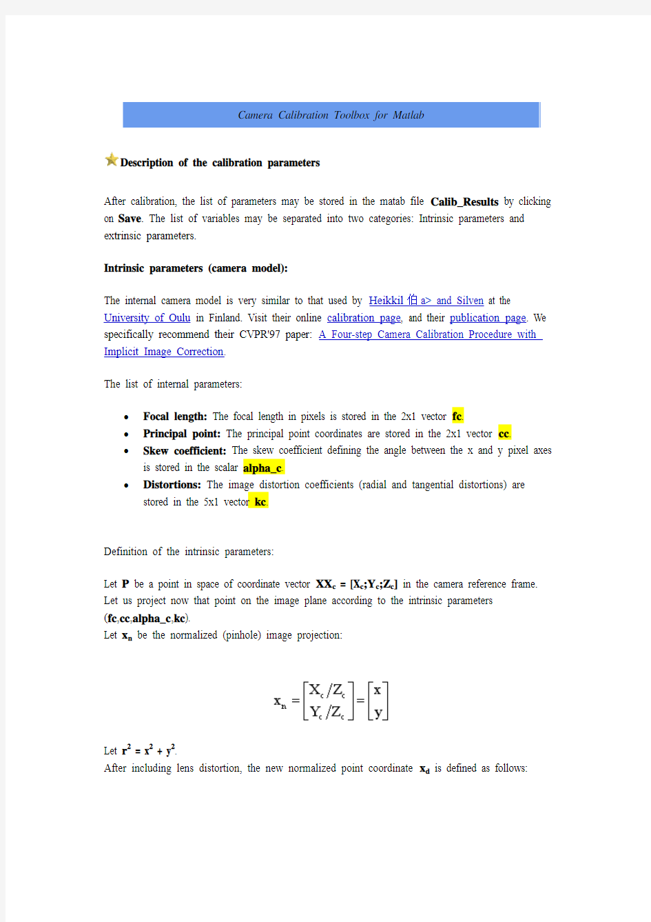
Let x n be the normalized (pinhole) image projection:

Let r2 = x2 + y2.

After including lens distortion, the new normalized point coordinate x d is defined as follows:

where dx is the tangential distortion vector:

Therefore, the 5-vector kc contains both radial and tangential distortion coefficients (observe that the coefficient of 6th order radial distortion term is the fifth entry of the vector kc).

It is worth noticing that this distortion model was first introduced by Brown in 1966 and called "Plumb Bob" model (radial polynomial + "thin prism" ). The tangential distortion is due to "decentering", or imperfect centering of the lens components and other manufacturing defects in a compound lens. For more details, refer to Brown's original publications listed in the reference page.

Once distortion is applied, the final pixel coordinates x_pixel = [x p;y p] of the projection of P on the image plane is:

Therefore, the pixel coordinate vector x_pixel and the normalized (distorted) coordinate vector x d are related to each other through the linear equation:

where KK is known as the camera matrix, and defined as follows:

In matlab, this matrix is stored in the variable KK after calibration. Observe that fc(1) and fc(2) are the focal distance (a unique value in mm) expressed in units of horizontal and vertical pixels.

Both components of the vector fc are usually very similar. The ratio fc(2)/fc(1), often called "aspect ratio", is different from 1 if the pixel in the CCD array are not square. Therefore, the camera model naturally handles non-square pixels. In addition, the coefficient alpha_c encodes the angle between the x and y sensor axes. Consequently, pixels are even allowed to be

non-rectangular. Some authors refer to that type of model as "affine distortion" model.

In addition to computing estimates for the intrinsic parameters fc, cc, kc and alpha_c, the toolbox also returns estimates of the uncertainties on those parameters. The matlab variables containing those uncertainties are fc_error, cc_error, kc_error, alpha_c_error. For information, those vectors are approximately three times the standard deviations of the errors of estimation.

Here is an example of output of the toolbox after optimization:

In this case fc = [657.30254 ; 657.74391] and fc_error = [0.28487 ; 0.28937], cc = [302.71656 ; 242.33386], cc_error = [0.59115 ; 0.55710], ...

Important Convention: Pixel coordinates are defined such that [0;0] is the center of the upper left pixel of the image. As a result, [nx-1;0] is center of the upper right corner pixel, [0;ny-1] is the center of the lower left corner pixel and [nx-1;ny-1] is the center of the lower right corner pixel where nx and ny are the width and height of the image (for the images of the first example,

nx=640 and ny=480). One matlab function provided in the toolbox computes that direct pixel projection map. This function is project_points2.m. This function takes in the 3D coordinates of a set of points in space (in world reference frame or camera reference frame) and the intrinsic camera parameters (fc,cc,kc,alpha_c), and returns the pixel projections of the points on the image plane. See the information given in the function.

The inverse mapping:

The inverse problem of computing the normalized image projection vector x n from the pixel coordinate x_pixel is very useful in most machine vision applications. However, because of the high degree distortion model, there exists no general algebraic expression for this inverse map (also called normalization). In the toolbox however, a numerical implementation of inverse mapping is provided in the form of a function: normalize.m. Here is the way the function should be called: x n = normalize(x_pixel,fc,cc,kc,alpha_c). In that syntax, x_pixel and x n may consist of more than one point coordinates. For an example of call, see the matlab function

compute_extrinsic_init.m.

Reduced camera models:

Currently manufactured cameras do not always justify this very general optical model. For example, it now customary to assume rectangular pixels, and thus assume zero skew (alpha_c=0). It is in fact a default setting of the toolbox (the skew coefficient not being estimated). Furthermore, the very generic (6th order radial + tangential) distortion model is often not considered completely. For standard field of views (non wide-angle cameras), it is often not necessary (and not recommended) to push the radial component of distortion model beyond the 4th order (i.e. keeping kc(5)=0). This is also a default setting of the toolbox. In addition, the tangential component of distortion can often be discarded (justified by the fact that most lenses currently manufactured do not have imperfection in centering). The 4th order symmetric radial distortion with no tangential component (the last three component of kc are set to zero) is actually the distortion model used by Zhang. Another very common distortion model for good optical systems or narrow field of view lenses is the second order symmetric radial distortion model. In that model, only the first component of the vector kc is estimated, while the other four are set to zero. This model is also commonly used when a few images are used for calibration (too little data to estimate a more complex model). Aside from distortions and skew, other model reductions are possible. For example, when only a few images are used for calibration (e.g. one, two or three images) the principal point cc is often very difficult to estimate reliably . It is known to be one of the most difficult part of the native perspective projection model to estimate (ignoring lens distortions). If this is the case, it is sometimes better (and recommended) to set the principal point at the center of the image (cc = [(nx-1)/2;(ny-1)/2]) and not estimate it further. Finally, in few rare instances, it may be necessary to reject the aspect ratio fc(2)/fc(1) from the estimation. Although this final model reduction step is possible with the toolbox, it is generally not recommended as the aspect ratio is often 'easy' to estimate very reliably. For more information on how to perform model selection with the toolbox, visit the page describing the first calibration example.

Correspondence with Heikkil?notation:

In the original Heikkil?paper, the internal parameters appear with slightly different names. The following table gives the correspondence between the two notation schemes:

A few comments on Heikkil?model:

?Skew is not estimated (alpha_c=0). It may not be a problem as most cameras currently manufactured do not have centering imperfections.

?The radial component of the distortion model is only up to the 4th order. This is sufficient for most cases.

?The four variables (f,Du,Dv,su) replacing the 2x1 focal vector fc are in general impossible to estimate separately. It is only possible if two of those variables are known

(for example the metric focal value f and the scale factor su). See Heikkil?paper for

more information.

Correspondence with Reg Willson's notation:

In his original implementation of the Tsai camera calibration algorithm, Reg Willson uses a different notation for the camera parameters. The following table gives the correspondence between the two notation schemes:

Willson uses a first order radial distortion model (with an additional constant kappa1) that does not have an easy closed-form corespondence with our distortion model (encoded with the coefficients kc(1),...,kc(5)). However, we included in the toolbox a function called

willson_convert that converts the entire set of Willson's parameters into our parameters (including distortion). This function is called in another function willson_read that directly loads in a calibration result file generated by Willson's code and computes the set parameters (intrinsic and extrinsic) following our notation (to use that function, first set the matlab variable calib_file to the name of the original willson calibration file).

A few extra comments on Willson's model:

?Similarly to Heikkil?model, the skew is not included in the model (alpha_c=0).

?Similarly to Heikkil?model, the four variables (f,sx,dpx,dpy) replacing the 2x1 focal vector fc are in general impossible to estimate separately. It is only possible if two of

those variables are known (for example the metric focal value f and the scale factor sx).

Extrinsic parameters:

?Rotations: A set of n_ima 3x3 rotation matrices Rc_1, Rc_2,.., Rc_20 (assuming n_ima=20).

?Translations: A set of n_ima 3x1 vectors Tc_1, Tc_2,.., Tc_20 (assuming n_ima=20). Definition of the extrinsic parameters:

Consider the calibration grid #i (attached to the i th calibration image), and concentrate on the camera reference frame attahed to that grid.

Without loss of generality, take i = 1. The following figure shows the reference frame (O,X,Y,Z) attached to that calibration gid.

Let P be a point space of coordinate vector XX = [X;Y;Z] in the grid reference frame (reference frame shown on the previous figure).

Let XX c = [X c;Y c;Z c] be the coordinate vector of P in the camera reference frame.

Then XX and XX c are related to each other through the following rigid motion equation:

XX c = Rc_1 * XX + Tc_1

In particular, the translation vector Tc_1 is the coordinate vector of the origin of the grid pattern (O) in the camera reference frame, and the thrid column of the matrix Rc_1 is the surface normal vector of the plane containing the planar grid in the camera reference frame.

The same relation holds for the remaining extrinsic parameters (Rc_2,Tc_2), (Rc_3,Tc_3), ... , (Rc_20,Tc_20).

Once the coordinates of a point is expressed in the camera reference frame, it may be projected on the image plane using the intrinsic camera parameters.

The vectors omc_1, omc_1, ... , omc_20 are the rotation vectors associated to the rotation matrices Rc_1, Rc_1, ... , Rc_20. The two are related through the rodrigues formula. For example, Rc_1 = rodrigues(omc_1).

Similarly to the intrinsic parameters, the uncertainties attached to the estimates of the extrinsic parameters omc_i, Tc_i (i=1,...,n_ima) are also computed by the toolbox. Those uncertainties are stored in the vectors omc_error_1,..., omc_error_20, Tc_error_1,..., Tc_error_20 (assuming

n_ima = 20) and represent approximately three times the standard deviations of the errors of estimation.

Back to main calibration page