Vol II-Chapter 11 Examples

Example 11.1 Calculation of Weibull Distribution Parameters for an Uncensored Sample Using the Maximum Likelihood Method

Problem Statement

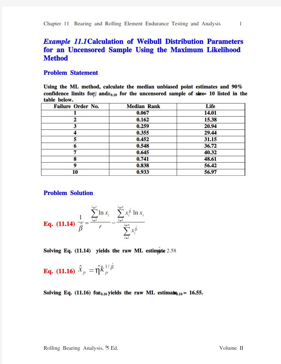
Using the ML method, calculate the median unbiased point estimates and 90%

confidence limits for β and x 0.10 for the uncensored sample of size n = 10 listed in the table below.

Failure Order No. Median Rank Life

1 0.067 14.01

2 0.162 15.38

3 0.259 20.9

4 4 0.35

5 29.44 5 0.452 31.15

6 0.548 36.72

7 0.645 40.32

8 0.741 48.61

9 0.838 56.42 10 0.933 56.97

Problem Solution

Eq. (11.14) ∑∑∑======?

i i i

n i i i

i r

i i i

x x r

x 1

ln ln ?1

βββ

Solving Eq. (11.14) yields the raw ML estimate 58.2?=β

Eq. (11.16)

η?/1??p p k x

Solving Eq. (11.16) for x 0.10 yields the raw ML estimate x 0.10 = 16.55.

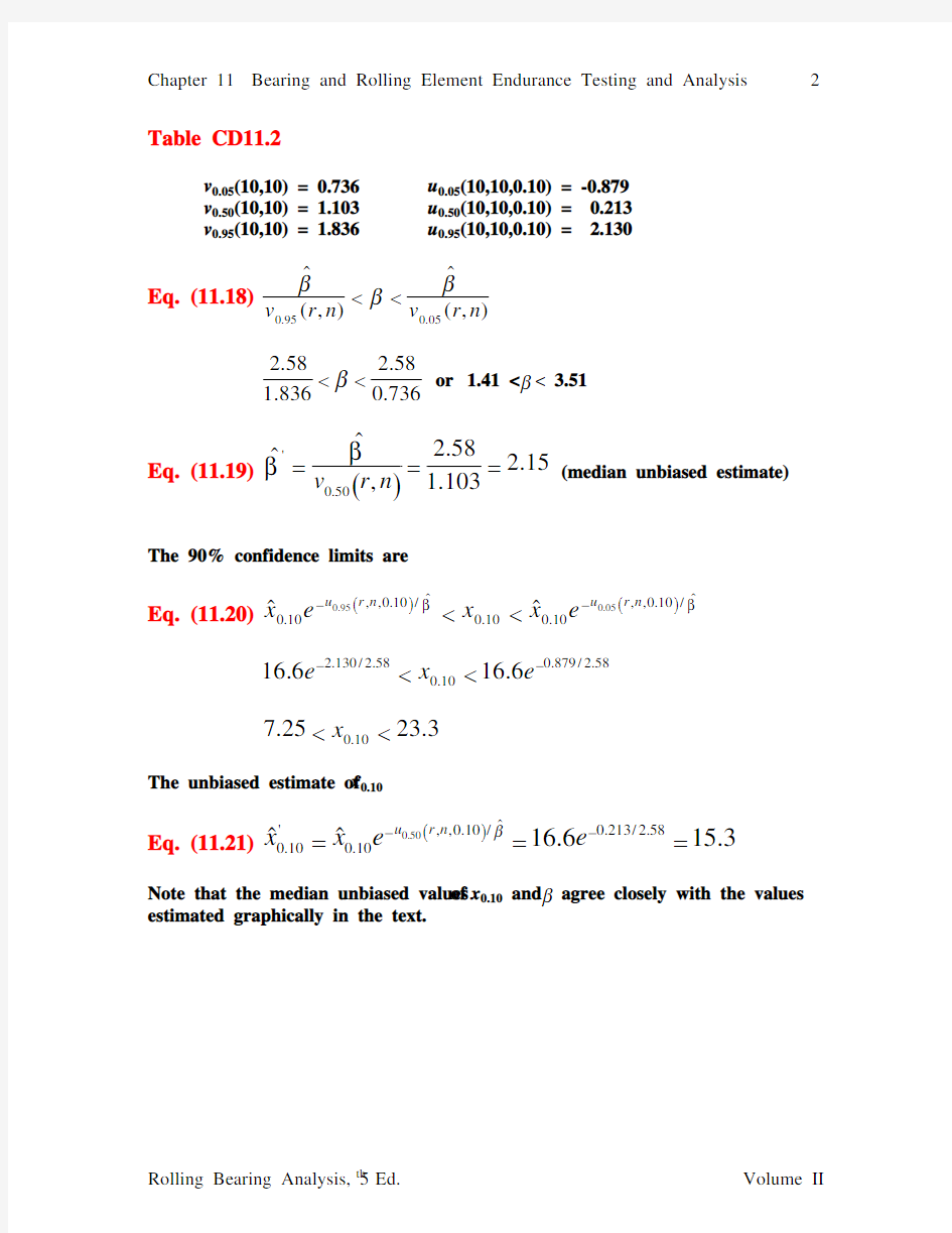
Table CD11.2

v 0.05(10,10) = 0.736 u 0.05(10,10,0.10) = -0.879 v 0.50(10,10) = 1.103 u 0.50(10,10,0.10) = 0.213 v 0.95(10,10) = 1.836

u 0.95(10,10,0.10) = 2.130

Eq. (11.18)

)

,(?)

,(?05.095.0n r v n r v βββ<

736

.058.2836.158.2<<β or 1.41 < β < 3.51

Eq. (11.19) ()15.2103

.158.2,??50.0'

===n r v β

β (median unbiased estimate)

The 90% confidence limits are

Eq. (11.20) ()()ββ

/10.0,,10.010.0?/10.0,,10.005.095.0??n r u n r u e x

x e x

??<<

58.2/879.010.058.2/130.26.166.16??<

3.2325.710.0<

The unbiased estimate of x 0.10

Eq. (11.21) ()3.156.16??58.2/213.0?/10.0,,10.0'10.050.0===??e e x

n r u β

Note that the median unbiased values of x 0.10 and β agree closely with the values estimated graphically in the text.

Example 11.2 Calculation of Weibull Distribution Parameters for the Results of Sudden Death Endurance Testis

Problem Statement

A sudden death test conducted with l = 3 subgroups, each of size m = 10, yielded the following values for the subgroup first failures: 4.72, 6.64, and 14.17. Determine the median unbiased estimates of the Weibull distribution shape parameter, 10% failure life, and 90% confidence limits on each.

Problem Solution

Eq. (11.14) ∑∑∑======?

i i i

n i i i

r i i i

x x

x 1

ln ln ?1

βββ

Solving Eq. (11.14) yields the raw ML estimate 27.2?=β

Eq. (11.16)

η?/1??p p k x

Solving Eq. (11.16) for x 0.10 yields the raw ML estimate x 0.10 = 3.59

Table CD11.3

q 0.05(3,10) = -2.91 v 0.05(3,3) = 0.650 q 0.50(3,10) = -0.133 v 0.50(3,3) = 1.53 q 0.95(3,10) = 1.83

v 0.95(3,3) = 5.71

Eq. (11.19) ()48.153

.127

.2,??50.0'

===l l v β

β (median unbiased estimate)

90% Confidence Limits on β

Eq. (11.18)

)

,(?)

,(?05.095.0l l v l l v βββ<

650

.027.271.527.2<<β or 0.398 < ? < 3.50

The unbiased estimate of x 0.10

Eq. (11.24) 34.99.9??27.2/133.0?/10.0'10.050.0===??e e x

q β

The 90% confidence limits are

Eq. (11.23) ()()β

?/10.0,,10.010.0?/10.0,,10.005.095.0??m l q m l q e x

x e x

??<<

27.2/91.210.027.2/83.19.99.9e x e <

6.3543.410.0<

Example 11.3 Estimation of Weibull Distribution Parameters for Multiple Sets of Data

Problem Statement

Ten bearings are fabricated from each of five different steel alloys. Uncensored life tests are performed on each bearing set. The raw maximum likelihood estimates of β and x 0.10 for each group are given by the table below:

Group No. 1 2 3 4 5

? 2.59 2.32 3.13 1.94 3.65 10.0?x 5.06 2.60 4.72 3.49 8.83 Determine which bearing sets differ significantly from the group.

Problem Solution

To determine whether a common Weibull shape parameter β is plausible, the ratio of the largest to the smallest shape parameter estimates is calculated. 88.194

.165.3??min max

===ββw

Table CD11.5 for n = r = 10 and k = 5, v 0.90 = 2.61

Since 1.88 < 2.61, the data are consistent with the assumption of constant β.

Eq. (11.26) ∑∑∑

∑∑==========?+k i i r j j k

i i n j j j i n j j j i j i j i x k x x

x rk 11

)

(?)()(1

ln ln 1?1βββ

ML estimate

48.2?1

=β

Eq. (11.30) 1

?/1??βηk x

i pi =

Eq. (11.31) 1

05.011

95.01?/)(10.0010?/)(10.0??ββu u e x

x e x

??<<

Eq. (11.32) 1

50.01?/)(10.0'10.0??βu e x

Recalculating i x

10.0?using Eq. (11.30), 90% confidence limits using (11.31), and median unbiased estimates '

10.0?x using (11.32):

Group No.

1 2 3 4

5 Raw ML estimate 10.0?x

4.84 2.81 3.80 4.87 6.34 Median unbiased estimate i x

10.0? 4.55 2.65 3.57 4.58 5.97 Lower confidence limit 3.25 1.89 2.55 3.27 4.25 Upper confidence limit

6.13 3.56 4.82 6.18

8.04

Table CD11.5 90th percentile of t 1(10,10,5) = 1.26

The shortest ratio of raw '10.0?x values that will be significant, denoted SSR (shortest

significant ratio) is defined implicitly by )ln(480.2)ln(?26.11

SSR SSR ==β

66.148

.2/26.1==e SSR

Thus, groups for which the ratio of raw ML estimates of x 0.10 exceeds 1.66 may be declared different. This would include groups 5 and 3, because their because their raw x 0.10 estimates are in the ratio 6.34/3.80 = 1.67 > 1.66. It is noted that the

confidence limits on x 0.10 overlap for these two groups. In general, if the confidence limits do not overlap, the groups differ. However, the groups may differ as in this example, even though the confidence limits do overlap.