jason_invermod
JASON 应用流程
地震数据加载
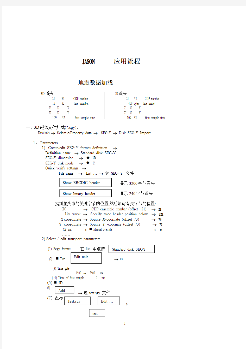
3D 道头 2D 道头
21 32 CDP number 21 32 CDP number
13 32 line number 400 bytes line name
73 32 X 73 32 X
77 32 Y 77 32 Y
109 32 first sample time 109 32 first sample time
一、3D 磁盘文件加载(*.sgy):
Datalinks → Seismic/Property data → SEG-Y → Disk SEG-Y Import …
1、 Parameters …
1) Create/edit SEG-Y format definition …→
Definition name → Standard disk SEG-Y
SEG-Y dimension → 3D
SEG-Y disk mode → C
Quick verify settings →
File name → List … → 选 SEG- Y 文件
显示3200字节卷头
显示240字节道头
找到道头中的关键字节的位置,然后填写有关字节的位置:
CDP → CDP ensemble number (offset 21) → 21
Line number → Specify trace header position below → 221
X coordinate → Source X-coornate (offset 73) → 73
Y coordinate → Source Y -coornate (offset 73) → 77
XY unit → Manual override → m
……
2) Select / edit transport parameters …
(1) Segy format 在 list 中点按 (2) → us
(3) Time gate
1500 --- 3500 ms
( 4) Time of first sample 0 ms
(5) 3D
→ 选 test.sgy 文件
(7)点按→
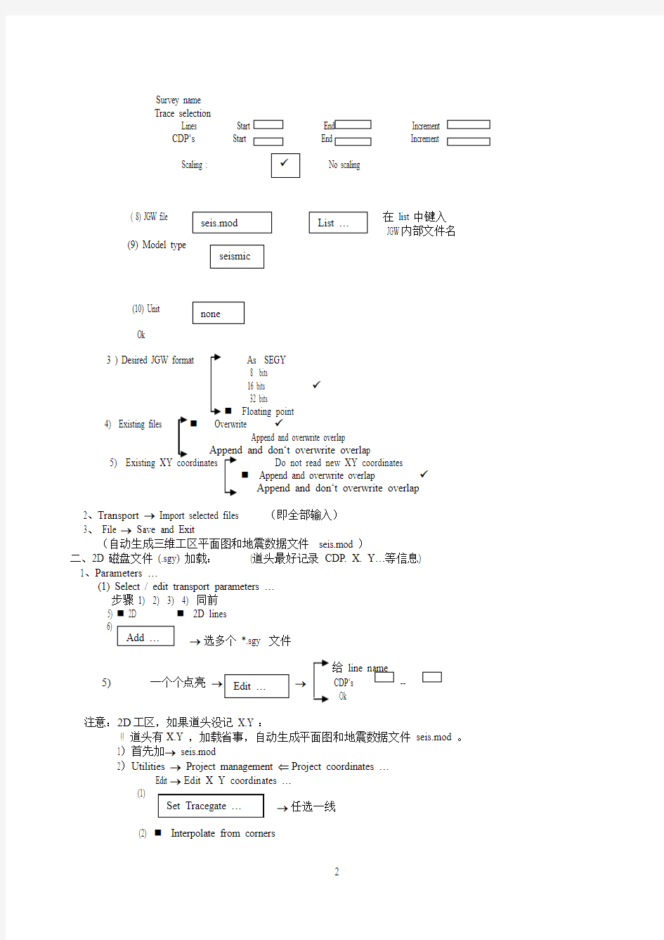
Survey name
Trace selection
CDP‘s
在 list 中键入 内部文件名
(10) Unit
Ok
?
Floating point
Overwrite ?
p
Append and overwrite overlap ?
Append and don‘t overwrite overlap
2、Transport → Import selected files (即全部输入)
3、 File → Save and Exit
(自动生成三维工区平面图和地震数据文件 seis.mod )
二、2D 磁盘文件 (.sgy) 加载: (道头最好记录 CDP. X. Y…等信息)
1、Parameters …
(1) Select / edit transport parameters …
步骤 1) 2) 3) 4) 同前
5) 2D 2D lines
→ 选多个 *.sgy 文件
给5) 一个个点亮 →--
注意:2D 工区,如果道头没记 X.Y :
!! 道头有X.Y ,加载省事,自动生成平面图和地震数据文件 seis.mod 。
1)首先加→ seis.mod
2)Utilities → Project management ? Project coordinates …
Edit → Edit X Y coordinates …
→ 任选一线
(2) Interpolate from corners
→
输入坐标
(3)
(1)(2) (3) 反复做,把所有的测线坐标输入进去。
(4)File → Save and Exit
井数据加载
一、 加载井曲线与井位(逐口井分别输入):
1、LAS 格式或ASCII 文件:
ASCII 文件 w01.asc
2、Datalinks → Wells → Well log import (las,ASCII)…
(1)Input → Set template file …→ 选井曲线数据文 → Ok
(2) Input → Select files…→ 选井曲线数据文件 → Ok
(3)Edit → Edit template …
注意深度单位
注意未定义数值的表示形式) 注意深度单位
Manual
注意深度单位 Manual
可以看文件头的内容
f)逐列编辑
选一个log → Edit header …
Ctrl + 选另一个 Type → 选另一个 log → Edit header…
注意:1) Depth: Ttack mode → Track only
2) 其他曲线 :Track mode → log only
3) 注意单位
(4) Edit → Overwrite
Append and don‘t overwrite overlap
(5) Transport → Import selected wells …
a) 任选一行
b) Edit …→
中键入井名
X coord
(补心海拔高与地震基准面海拔值的高差)
( Datum
给零值,通过时深 tops 确定 Datum )
Ok
d) Ok
(6) File → Save and Exit (一定要先存
,后退出)
3、显示井位:
Analysis → Map view and calculations …
在 Map view 窗口检查井位
Input → Wells → Use Time as Vertical axis? (no) (用深度域显示)
→ 选 *.wll → Ok
二、斜井轨迹加载:(在4.x 版本中,斜井的深度必须用TVD)
1、> vi deviate.dat
σx. σy 为相对井口的坐标位移)
步骤与前相同,至少三行数据。
2、注意:
1) 井曲线要与目的层位相交
2) 井曲线加载后再加井轨迹 (直井就不用加井轨迹)
3) 先在深度域显示井位.井轨迹和井曲线(检查)
深度域剖面显示:
Applications → Display & Editors
→ section visualization and interpretation …
Input → Vertical gate …→ Depth …→ 选深度范围
Input → Wells …→ no → 选深度域井文件→ 选井曲线
Display track Display tops
三 、井分层数据与时深关系的加载:
1、 > vi well.top (多井自由格式)
注意:1) 注意单位: depth : m time : s
2) Top name 与层名 (horizon name)要一致
2、Datalinks → Wells → Well tops import (ASCII) …
(1) Input → ASCII well tops file …→ 选 tops 文件
(2) Input →Parameters …→
空白
― ‖
― ―
? ?
给 top name
所在列数
给 well name 所在列数
给 time 所在列数
时间单位
给
depth 所在列数
深度单位
→
*.tpl
6) Ok
(3) Input → 中修改井名.wll
键入X .Y 坐标
给零值
(4) Existing files →?
(5) Transport → Import
3、在平面和剖面图窗口上显示深度域的 tops (检查)
4、File → Save and Exit
四、 增加井曲线类型及其单位:
Utilities → Project management → Project parameters …
1、Edit → Type and units …
Unit :
或者 Data ytpe :
Unit :
ν Lithologic data type :
→
Litho-type :
Integer representation :
……(例如 : sand 1, oil-sand 2, …)
逐个键入,Ok
2、File → Save and Exit
增加的内容存在文件 usertypelist.txt 中
Horizon data Export & Import
一、Export (Geoquest) horizons … (3D )
Datalinks → Geoquest IES(x) → Horizons export …
1、> geohorsexp . input.hor (input.hor 为JGW 的层位文件名)
2、Enter Geoquest card image format :
1:
…
5: P7 (Multi horizon 3D)
6: P7 (Multi horizon 2D)
Enter your choice :5 ( p7(Multi horizon 3D) (选输出格式) )
3、Enter name Geoquest file ( without extension ) : (给输出文件名)
geo
(显示Trace gate)
4、Use this tracegate (YN) y
5、 Enter element to store JGW trace number in :
1) trace numbers
2)CDP numbers
3)shotpoints
4)x position
5)y position
Enter your choice : 1
6、层位文件列表: (选层号)
Enter number to (De) select horizon ( 0:ready) : 1
Enter the geoquest unit (s) : ms (注意用 ms)
Enter the geoquest column in which to output ( 1=Time, 2=Amplitude) (1) : 1
(反复选层)
7) Enter number to (De) select horizon ( 0=ready) : 0
( 生成 geo.p701 )
二、 Import horizons ( 3D ) 注意单位( ms )
Datalinks → Geoquest IES(x) → Horizons import …
1、Input :
(1) Geoquest files …→ gqs.p701 (2) Horizons …→ 选输入的层名 →(3)
→→ Ok (注意用 ms)
(4) Line / traces …→ none ( ) → Ok (注意 trace gate skip ?, and survey name)
(不用编辑 attribute unit: )
2、Options …→
(1) File type
X Y unit : m
观察数据)
(2)→
Append and don‘t overwrite overlap
3、→ Import selected horizons …
→ 键入 input.hor (给JGW 文件名)
→ Ok
VelMod
一、迭加速度文件:
1、二维速度谱数据:HANDVEL-- 2D 格式(每八列一个数,数据右对齐)
时间ms 速度m/s
2、三维速度谱数据:HANDVEL —3D 格式(每八列一个数,数据右对齐)
二、迭加速度输入 :
DataLinks → Velocity data …(Import ascii Velocity files )
1、 Parameters …
(1) Select / edit transport parameters …
Time
Velocity unit of input files : ms
2D
2D lines
→ 选迭加速度文件 ( vel836.dat )
照亮文件名→→ 改测线名
JGW velocity file :
Model type :
Sample interval : 2 ms
Ok
(2)Desired JGW format
(3)Existing file :
(4) Existing XY coordinates :
2、 Transport → Import selected file …
3、File → Save & Exit
4、剖面检查迭加速度 :如果个别速度谱不好,可在原始文件中去掉 个别速度谱,再重新输入。
三、转换层速度 :
VelMod → Velocity conversion …
1、Input:
(1) Stacking velocity data …→ stack_velocity.mod
(2) Trace gate …
2、Edit → Datum
Use constant time datum
Constant time datum (0) : 0
3、Output → Generate …
Instanteous velocity
4、File →
Save & Exit
5、剖面检查层速度 :可对层速度进行平滑,中值滤波,或带通滤波处理,
以改善层速度的质量。
四、建地层构架表;
VelMod → Model builder ( without TDC )
1、Input :
(1) Time / Depth mode …→ Time
(2) Horizons …→ 选层文件
(3) Tramework …( 第一次作,不用选此项)
(4) Trace gate … (注意:线和道 skip=0,或与工区定义的要一样)
2、Edit …
(1) Edit framework …
(2) Edit data for EarthModel → Areal weight interpolation :
( Locally weighted or locally weighted & trianglation )
3、Output → Generate …(主要是产生内插的层)
Run now
选输出内容: *.h*
4、file → Save & Exit
五、层速度编辑:
VelMod → Property conditioning …
1、Input :
(1) Time / Depth mode …→ Time
(2) solid model …→ vel
(3) Seismic / Property data …→ vi_time.mod
(4) Trace gate …
(5) Datum parameters …→
Use constant time datum
Constant time datum (s) : 0
2、Edit … (分层编辑层速度):
(1) Scatter correction …
Select layers …
Left … jump
Right … jump
Apply
…… ( 逐层编辑层速度范围,去掉奇异值)
Done
(2)
Inline
Crossline
3、Output :
(1) QC panel → (检查层速度的编辑是否合理)
(2) Generate …
Seismic / Property file 4、File → Save & Exit
六、速度谱内插:
VelMod → Model interpolator …
1、Input:
(1) Time/Depth mode → Time
(2) Solid model → Vel
(3) Layers … → 选
(4) Data for seismic modeling → Tpropcond.mod ( 编辑后的层速度体)
(5) Trace gate → Input trace gate → 选,(注意原始速度谱点的 skil 数)
例如: line CMP
20 140
35 179
skip 14 38
Output trsce gate → 选,(注意要和工区定义的skip 数一样)
例如:line CMP
20 140
35 179
skip 0 0
2、Edit :
(1) Interpolation/extrapolation method → local …
(2) Interpolation parameters :
Max interpolation distance : 1000 (速度谱点之间的距离)
Lteral interpolation : horion fitting
Time sample interval : 4 ms
Vertical interpolation property data : blocking
3、Output → Generate
Run now
→ interpolation_Tvelocity.mod
Timpedance _from_velocity.mod
Timpedance_from_gardner.mod
Tsonic_from_velocity.mod
……
七、建立伪井,并从数据体中提取多种曲线 :
Analysis → Well log editing and seismic tie …
1、Output → Create pseudo.wll
Well file :
键入坐标)
→ *Timpedance_from_velocity.mod
Tsonic.mod
Tvelocity.mod (提取伪井的曲线logs)
……
Horizon file :
tops
)
2、平面图显示伪井井位
3.、剖面图显示提取的曲线
** 应用方法:
1.、编辑原始叠加速度。
2、分层编辑层速度,可作平滑处理。
3、可对 Tvelocity ,Timpedance …作低通滤波,(层速度低通 (0,3)HZ )。
4、可对 Tvelocity ,Timpedance …作中值滤波。
Well Edit 、TDC & Synthetics
一、深度域井曲线编辑:
Analysis → Well log editing and seismic tie …
(1) Input → Well… ? *.wll (选深度域井文件)
(2) 选曲线显示 (p_sonic,density,…)
(3)编辑井曲线:(按右键,选择编辑功能)
a) 消除奇异值,
b)延长曲线。
具体方法:
右键 → Draw log
用右键选被编辑的曲线,用左键画曲线,
点按
(4) 若没有密度曲线: 点按 (5)计算深度域阻抗曲线,点按
(6)→ p_Impedance
(6) (7)
二、直接将深度域曲线转为时间域:
在
点按
→ 给一对合理的时深数据
→ Display → Well vertical type → Time
(窗口显示时间域曲线)→ 选层
Save as … → *_T1.wll
三、 作初始雷克子波: 初步 调整Tops 与Horizons 的关系:
Modeling → Wavelets
1、输入有关参数:
Input → Seismic mode …→ Zero offset
AVA
Input → seismic → seismic data … → 选地震数据
Input → Wells/User locations → Select well …→ *T1.wll
(选经过深时转换的井文件)
Input → Time gate …→ … (选子波估算的时窗)
Input → Select traces… (选井旁道,最好选走向方向的井旁道)
投影距离
2、Edit →
Wavelet
L ength (s) :
显示子波波形、振幅谱与相位谱
不断调整子波主频、与地震频谱对比
OK
3、 然后在Well log editing and seismic tie 中:
Input → Seismic data …→ seismic.mod
Input → Wavelet → 选子波,(选 Create_wavelet.mtr )
用此子波调整分层(tops)与地震解释(horizons)的关系
Edit mode : Bulk shift all
Stretch / squeeze all
Edit → Scale wavelet …
(注意:雷克子波的振幅与井旁地震道振幅不匹配,
必须计算子波的比例因子。)
反复调,…
Save as …→ *T2.wll
四、从地震数据中估算子波------ 制作合成记录:
Input → Seismic data …→ seismic.mod
Input → Wells/User locations → Select well …→ *T2.wll
(选经过再一次时间调整的井文件)
Estimate → Estimate wavelet amplitude and phase spectra …
振幅谱斜坡的衰减类型)
Output wavelet
Length(s):
Wavelet maximum frequency (HZ):
OK
然后在 Well log editing and seismic tie …中:
Input → Wavelet → amp+phase_wavelet.mtr
反复调整合成记录,在调整过程中,要显示以下曲线:
Select logs … → p_sonic
Time (慢度曲线,用于调整合成记录的质量控制)
P_impedance(置为当前曲线)
→ *T3.wll
!!不断重复以上过程,直到子波形状规则、旁瓣小、tops 与horizons 对齐、
合成记录的主要目的层与地震记录一致为止。
五、子波提取中要注意的问题:
1、子波长度:
太长不好,视地震的频带宽度而定,一般为100ms 左右为宜,保证一个主瓣和两个旁瓣。
2、制作子波的时窗(time gate):
1)时窗不能太小,至少是子波长度的三倍以上,注意时间不要卡在强轴上,要定在地震 波的过度带上。
2)当目的层较深、地震资料的信噪比较低时,提取子波的时窗最好用浅层部分为好,
因为浅层资料频率损失较少;而深层资料频率损失严重, 主频太低,影响地震反演效果。
3)提取子波的时窗,也可以以目的层为中心,
其上取 0.05ms
其下取 0.05ms
Input → Ti me gate …
Use horizons
→ *Tinterface.hor
Offset from top horizon(s):
Offset from bottom horizon(s) :
注意不要卡在强轴上!
4) 井旁道数扫描,至少为三道,道数太少,估算的子波不稳定。最好为走向方向.
5)第一次的合成记录用雷克子波,
主要目的是把地震解释的层位与井分层对齐 。
后边的合成记录用从地震数据中提取的子波,不断调整合成记录的波形、振幅 与时间。
6)子波的比例因子 至关重要:
因为在所有的反演算法中,均以合成记录代替地震数据进行计算,因此必须保证合成 记录与地震数据的最大匹配,使剩余值更少些。
子波比例的调整方法:
(1) Edit → Scale wavelet …
(2_ InverTrace → CSSI → Edit → Wavelet scaling …
Input wavelet
Output wavelet
选择,如果比例因子接近1,则应用的子波是 amp+phase_wavelet.mtr
如果子波比例因子变化大,应在 Input 中重新选比例后的
子波 amp+phase_wavelet _scale.mtr
六、修正调整后的深度域 p_sonic 曲线:
井的时深关系、合成记录与子波均调整好后 ,如果时间域声波曲线修改较大,
则:
Analysis → Well lig editing and seismic tie → (进入时深显示状态)
→ *_calibri.wll
EarthModel builder with TDC 模块。
七、显示各次作的子波:
Analysis → Graph view …
Input → Single trace …
→选子波(对比多次提取的子波, 不用 *last.mtr )
→选 0 (最长的子波)
Earth Model (EM )
必备条件:
1、深度域的 tops、 logs 和时间域的 Horizons
2、top name & horizon name 要一样
3、顶层和底层必须解释,各层都有解释结果
4.、逆断层两侧的层名(horizon name)要不同,而地层介质名(layer name)要相同
5、Time-Depth的关系正确
首先作时间域的 EarthModel:
(一)EarthModel → Model builder ( without TDC ) Without TDC
1、Input :
(1)Horizons …→选层文件 input.hor(包括断层)
(2)Horizons / tops to tie …→ (选感兴趣的层,该层必须是井上分层和层文件都有的
相对应的层)
(3)Framework … →第一次做,可不选;如果已有 *.frm 文件,可选一个参考(*.frw)
(4) Wells …→选已经编辑调整好的深时转换的井文件(*T*.wll), ctrl +左键(选多井)
(5)Logs …→选多种井曲线
(只选三种: p_sonic,
density,
p_impedance)
(6)Trace gate …→选道范围
2、Edit:
(1) Edit framework … -------关键 ( *.frw )
注意:
a) 制表应注意的事项:
从底层开始向上逐层编辑
先建断层下盘的地层,后建断层上盘的地层
被断层切割的层不能作为 datum
有断层时最好加顶、底层
b)QC trace gate …(建立QC道范围)
Generate QC (计算)
QC panel ? (看地层构架表是否合理,便于再修改)
c)Save as …(*.frw)
d)Ok
(2)Edit data for EarthModel
选内插算法)
(井少时用此法)
→给每口井分配权,一般用1
Vertical detail : 4ms (要与地震数据的采样率一样)
(对每种曲线 定义时间域的垂向采样率 )
3、Output → Generate …
(1) λ Run now
(2) 选输出内容: (选* T interface.hor ) (选井、深度层、时间层)
(3) Output solid model :
Output directory:
产生文件: ../solid_notdc/Tinterface.h*
4、File → Save & Exit
5、剖面显示,检查时间域的 井曲线和分层数据
(二)EarthModel → Model generator … Without TDC
1、Input :
(1) Solid model …→ notdc (选 Model builder without TDC 的结果 )
(2) Trace gate …
2、Edit :
(1) Model parameters …
Time sample interval : 0.004 s
( 采样间隔:用于 InverTrace 时,采样间隔与地震一样。
310
0.25
(2) Edit data for seismic modeling :
Wavelet interpolation …→ 选内插算法
Time gate …→ Use horizons
Set horizons file … ? *Tinterface.hor
Top horizon
Bottom horizon
3、Output → Generate … (选 Timpedance.mod )----用于后边的Trace merging
然后作时间与深度转换的 EarthModel:
(一)EarthModel → Model builder ( with TDC ) TDC
1、Input :
(4) Horizons …→ 选层文件 input.hor (包括断层)
(5) Horizons / tops to tie …→ (选感兴趣的层,该层必须是井上分层和层文件都有的
相对应的层)
(6) Framework … → 第一次做,可不选;如果已有 *.frm 文件,可选一个参考(*.frw)
(4) Wells …→ 选已经编辑调整好的深时转换的井文件(*calibre.wll ), ctrl +左键(选多井)
(7) L ogs …→ 选多种井曲线
(8) Trace gate …→ 选道范围
2、Edit :
(1) Edit framework … -------关键 ( *.frw )
注意:
a) 制表应注意的事项:
从底层开始向上逐层编辑
先建断层下盘的地层,后建断层上盘的地层
被断层切割的层不能作为 datum
有断层时最好加顶、底层
c) QC trace gate … (建立QC 道范围)
Generate QC (计算)
QC panel → (看地层构架表是否合理,便于再修改)
c) Define datum … → *Time horizon
Depth from
e) Save as …(*.frw)
f)
Ok
(2)
Conversion parameters …
Standard deviation depth datum : 0
Standard deviation depth thickness : 6 (2)
Standard deviation sonic scale factor : 0.1
(3)Edit data for EarthModel and / or InverMod
选内插算法)
(井少时用此法)
→ 给每口井分配权,一般用1
Vertical detail : 2 m 1ms
(对每种曲线 定义垂向分辨能力 )
3、Output → Generate …
(3) Run now
(4) 选输出内容: (选* calibre.wll 、Tinterface.hor , Zinterface.hor )
(选井、深度层、时间层)
(3) Output solid model :
Output directory : solid_tdc
产生文件: *calibre.wll
Tinterface.h*
Zinterface.h*
4、File → Save & Exit
5、剖面显示,检查时间域的 井曲线和分层数据
(二)EarthModel → Model generator … TDC
1、Input :
(1) Solid model …→ tdc (选 Model builder with TDC 的结果 )
(2) Trace gate …
2、Edit :
(3) Model parameters …
Time sample interval : 0.001 s ( 0.0005)
( 采样间隔: 用于 InverMod 和 StatMod 时,采样间隔可小些。) Depth sample interval : 2 m 1ms
310
0.25
(4) Edit data for seismic modeling :
Wavelet interpolation …→ 选内插算法
Time gate …→ Use horizons
Set horizons file … *Tinterface.hor
Top horizon
Bottom horizon
3、Output →Generate …(选 *.mod)
Run now
任选输出内容: Timpedance_from_sonic.mod
Timpedance_from_sonic_and_density.mod
Timpedance_from_sonic_gardner.mod
Tporosity.mod
Tsonic.mod
Tdensity.mod
……
Zimpedance_from_sonic.mod
Zimpedance_from_sonic_and_density.mod
Zimpedance_from_sonic_gardner.mod
Zporosity.mod
Zsonic.mod
Zdensity.mod
……
*Ok
产生文件: ../solid_tdc/*.m*
4、File → Save & Exit
5 、在剖面和平面图窗口中查看结果:
检查 horions .tops .logs 三者合适,该结果的质量至关重要!!
内插的井曲线数据体的空间分布要合理,符合地质沉积规律。
三、EarthModel →Model interpolator … (常规流程不用作)
1、Input :
(1)Time / Depth mode …→ Time
(2)Solid model … → tdc1
(3)Layers …→选多层,给采样间隔
(4)Seismic /Property data …→ velocity.mod
(5)Trace gate … Input trace gate … (稀)
Output trace gate …(密)
2、Edit :
(1)Inter / extrapolation method …→选内插算法
(2)Interpolation parameters …
Time sample interval : 0.004 s 0.002 s
Maximum lateral interpolation distance : 25 m
?
?
3、Output →Generate …→ interpolate.mod
4、File → Save & Exit
Wavelets →Wavelet estimation … WE 一、有井,无井------估算雷克子波:
(一) Input :
1、Seismic data …→ seis.mod
2、Wells / User locations
有井: Use wells
Select wells → *.wll (选深时转换的井文件)
无井: User other location
Select location … (在平面图上选一点)
3、Solid model …→
Use solid model
Select solid model …→ tdc1
4、Time gate …
Use horizons
Set horizons file …→ *Tinterface.hor
Top horizon
Bottom horizon
5、Select traces …→ 选井旁地震道数
(二) Output → Create synthetic wavelet …
Wavelet type :
( Ricker
Ricker wavelet central frequency : 35 )
Double cosine ?
Low Opper Lower Upper
0 25 37.5 62.5
0 10 80 100
Start time : -0.03 Phase rotation : 0
Length : 0.06 Sample interval : 0.002
看QC
Ok
二、有井或无井时------从井旁道的地震数据中估算子波:
(一) Input :
Wells /User location …
有井: Use wells
Select wells → tdc1_tdc_*.wll (选深时转换的井文件) 无井: Use other location
Select location …
( 其他步骤同前 )
(二) Output → Estimate wavelet amplitude & phase spectra …
?(缓慢衰减)
Output wavelet
Wavelet start time : -0.064 -0.03
Wavelet length : 0.128 0.06
Wavelet maximum freq. : 100
( Wells correlation range (s) : 0.01
Use prior wavelet to stabiliz Yes No
Prior wavelet : wavelet-1.mtr
Prior wavelet weight : 0.1 )
QC
Ok
三、 File → Save & Exit
四、观察子波:
Applications → display & Editors →Graph visualization …
→ Input → Single trace …
→ 0
InverTrace
一、 InverTrace →Constrained sparse spike … CSSI---(约束稀疏脉冲反演)
1、Input :
(1)Seismic data and wavelets …→
Seismic → list …→ seis.mod
Select Wavelet …→ list …?选一个子波
(2)Trace gate …
(3)Time gate …→
Use horizons
Set horizons file …→ *Tinterface.hor
Top horizon
Bottom horizon
(4)Wells / User locations
Use wells
Select wells …→ (选多个时深转换的井文件)
(5)Select QC traces … (3-5道)
2、Edit :
(1)Edit trend :
Trend is : constrant
Horizonfile …→ *Tinterface.hor
Horizons …→选层
From log …→ (用多井阻抗曲线自动计算趋势)
编辑趋势(曲线中心)
Select well … (逐口井检查趋势,反复做)
Save as …→ *.atm ? Ok
(2)Edit constraints … (用井的阻抗曲线,约束地震反演的数据范围)
逐口井编辑约束带,把所有的井数据包括进去。
Save as …→ *.atm → Ok
(3)Wavelet scaling …
Output wavelet
Scale factor : 1
Save as …
注意:当经过子波比例因子的估算后,存了一个新的子波,这时需要回到 input 中重新选择经过子波比例后的新子波。
(4)Edit and QC parameters …
Lambda 5 50 35