Dispersion of tracer particles in a compressible flow

Dispersion of tracer particles in a compressible ?ow
John R. Cressman,1 Walter I. Goldburg,1 and J¨rg Schumacher2 o
1
Department of Physics and Astronomy, University of Pittsburgh, Pittsburgh, PA 15260, USA 2 Fachbereich Physik, Philipps-Universit¨t, D-35032 Marburg, Germany a (Dated: February 5, 2008)
arXiv:nlin/0402031v1 [nlin.CD] 19 Feb 2004
The turbulent di?usion of Lagrangian tracer particles has been studied in a ?ow on the surface of a large tank of water and in computer simulations. The e?ect of ?ow compressibility is captured in images of particle ?elds. The velocity ?eld of ?oating particles has a divergence, whose probability density function shows exponential tails. Also studied is the motion of pairs and triplets of particles. The mean square separation ?(t)2 is ?tted to the scaling form ?(t)2 ∝ tα , and in contrast with the Richardson-Kolmogorov prediction, an extended range with a reduced scaling exponent of α = 1.65 ± 0.1 is found. Clustering is also manifest in strongly deformed triangles spanned within triplets of tracers.
PACS numbers:
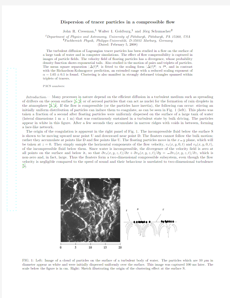
Introduction.— Many processes in nature depend on the e?cient di?usion in a turbulent medium such as spreading of drifters on the ocean surface [1, 2] or of aerosol particles that can act as nuclei for the formation of rain droplets in the atmosphere [3, 4]. If the ?ow is compressible (or the particles have inertia), the following can occur: stirring an initially uniform distribution of particles can induce them to coagulate, as can be seen in Fig. 1 (left). This photo was taken a fraction of a second after ?oating particles were uniformly dispersed on the surface of a large tank of water (lateral dimensions 1 m × 1 m) that was continuously sustained in a turbulent state by bulk driving. The particles appear in white in this ?gure. After a few seconds they accumulate in narrow ridges with voids in between, forming a lace-like network. The origin of the coagulation is apparent in the right panel of Fig. 1. The incompressible ?uid below the surface S is shown to be moving upward near point U and downward near point D. The ?oaters cannot follow the bulk motion; rather they accumulate at points like D and ?ee points like U. The ?oating particles move in the x?y plane, which will be taken at z = 0. They simply sample the horizontal components of the ?ow velocity, vx (x, y, 0, t) and vy (x, y, 0, t), of the incompressible ?uid below them. Since water is incompressible, the divergence of the velocity ?eld is zero at all points on the surface and below it, so that ?vx (x, y, z, t)/?x + ?vy (x, y, z, t)/?y = ??vz (x, y, z, t)/?z, which is non-zero and, in fact, large. Thus the ?oaters form a two-dimensional compressible subsystem, even though the ?ow velocity is negligible compared to the speed of sound and their behaviour is unrelated to two-dimensional turbulence [5].
FIG. 1: Left: Image of a cloud of particles on the surface of a turbulent body of water. The particles which are 10 μm in diameter appear as white and were initially dispersed uniformly over the surface. This image was captured 100 ms later. The scale below the ?gure is in cm. Right: Sketch illustrating the origin of the clustering e?ect at the surface S.

2 Recently, compressible turbulence has come under theoretical scrutiny (see [6] for a review). Modelling the ?ow as Gaussian and delta-correlated in time, one can show for both spatially smooth [7] and spatially rough ?ows [8], that a transition from a regime of weak to strong compressibility occurs at some threshold value of the dimensionless ratio, de?ned as C ≡ (?vi /?xi )2 / (?vi /?xj )2 , (1)
with i, j = 1, 2. Clearly, for any C = 0 tracers will cluster, but the eventual particle distribution will depend on whether C is above or below the threshold. Assumptions contained in those models make it inapplicable to the present experimental situation, where the ?ow is non-Gaussian and has a ?nite time correlation. Because the idealizations in those models are not realized in the experiment, we do not know if such a transition from weak to strong compressibility exists in our experiment. On the other hand, a computer simulation (DNS) that roughly matches the ?ow conditions of this experiment (incompressibility of the three-dimensional velocity ?eld at all z ≤ 0, ?nite correlation time, and a free-slip boundary condition at the ?at surface) are in remarkably good agreement with the ?rst experiments [9, 10]. Herein, we summarize and extend recent experiments using freshly cleaned water surfaces [11]. Our study focuses on two points. The ?rst one is the relative motion of the ?oaters, with special emphasis on so-called Richardson di?usion [12], which refers to the time dependence of the mean square particle separation ?(t)2 ～ tα with α = 3. Scaling close to the Richardson prediction was found in experiments [13] as well as in high-resolution numerical simulations [14] in the inverse cascade of two-dimensional incompressible turbulence. Intermittency e?ects if present seem to modify this exponent only slightly [15]. Dimensional arguments would seem to be inapplicable for the ?oaters, since they can exchange kinetic energy and mean square vorticity with the ?uid below them. Since a theory for their motion has yet to be developed, one must again turn to computer simulations, which have been recently carried out [16]. Secondly, ?rst studies the competing e?ects of coherent shear and random motion in the surface ?ow are presented by analyzing the evolution of shapes formed by three particles tracked simultaneously [17, 18]. By neglecting the center of mass,√ the relative position of three points can be conveniently expressed by the following two vectors, √ 2 a1 = (x2 ? x1 )/ 2 and a2 = (2x3 ? x1 ? x2 )/ 6 [18]. The distortion of a triangle is measured by the ratio I2 = g2 /R2 2 + a2 , to the smaller half-axis, g , of the smallest ellipse that covers the which relates its radius of gyration, R = a1 2 2 tracer triangle. From [18] we get for two dimensions I2 = 1 1? 2 1? 4 (a1 × a2 )2 R4 . (2)
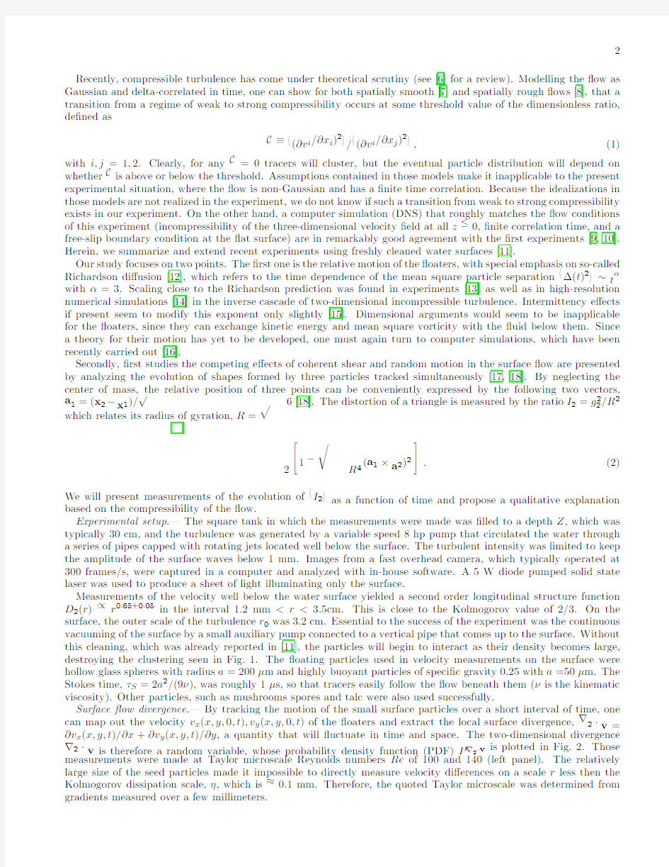
We will present measurements of the evolution of I2 as a function of time and propose a qualitative explanation based on the compressibility of the ?ow. Experimental setup.— The square tank in which the measurements were made was ?lled to a depth Z, which was typically 30 cm, and the turbulence was generated by a variable speed 8 hp pump that circulated the water through a series of pipes capped with rotating jets located well below the surface. The turbulent intensity was limited to keep the amplitude of the surface waves below 1 mm. Images from a fast overhead camera, which typically operated at 300 frames/s, were captured in a computer and analyzed with in-house software. A 5 W diode pumped solid state laser was used to produce a sheet of light illuminating only the surface. Measurements of the velocity well below the water surface yielded a second order longitudinal structure function D2 (r) ∝ r0.65±0.05 in the interval 1.2 mm < r < 3.5cm. This is close to the Kolmogorov value of 2/3. On the surface, the outer scale of the turbulence r0 was 3.2 cm. Essential to the success of the experiment was the continuous vacuuming of the surface by a small auxiliary pump connected to a vertical pipe that comes up to the surface. Without this cleaning, which was already reported in [11], the particles will begin to interact as their density becomes large, destroying the clustering seen in Fig. 1. The ?oating particles used in velocity measurements on the surface were hollow glass spheres with radius a = 200 μm and highly buoyant particles of speci?c gravity 0.25 with a =50 μm. The Stokes time, τS = 2a2 /(9ν), was roughly 1 μs, so that tracers easily follow the ?ow beneath them (ν is the kinematic viscosity). Other particles, such as mushrooms spores and talc were also used successfully. Surface ?ow divergence.— By tracking the motion of the small surface particles over a short interval of time, one can map out the velocity vx (x, y, 0, t), vy (x, y, 0, t) of the ?oaters and extract the local surface divergence, ?2 · v = ?vx (x, y, t)/?x + ?vy (x, y, t)/?y, a quantity that will ?uctuate in time and space. The two-dimensional divergence ?2 · v is therefore a random variable, whose probability density function (PDF) P?2 ·v is plotted in Fig. 2. Those measurements were made at Taylor microscale Reynolds numbers Re of 100 and 140 (left panel). The relatively large size of the seed particles made it impossible to directly measure velocity di?erences on a scale r less then the Kolmogorov dissipation scale, η, which is ≈ 0.1 mm. Therefore, the quoted Taylor microscale was determined from gradients measured over a few millimeters.

3
0
Experiment
0 Re=100 Re=140 ?1
DNS
Re=106 Re=157 Ref. [16]
?1
log10[Pdf(div)]
?2
log10[Pdf(div)] ?5 0 div/σ 5 10
?2
?3
?3
?4
?4
?5 ?10
?5 ?10
?5
0 div/σ
5
10
FIG. 2: Probability density function (PDF) of the surface ?ow divergence ?eld with σ = (? · v)2 1/2 . Left panel shows the experimental ?ndings for two Taylor microscale Reynolds numbers of Re = 100 and 140, respectively. Right panel shows the simulation results for three di?erent values. Runs at Re = 106 and 157 are for driving by a large-scale shear. Data from [16] were obtained with isotropic volume forcing at a Taylor Reynolds number of Re = 145.
New experimental data were extracted from an ensemble of measurements made at many instants of time and many points (x, y) in the surface. Note that the mean value of ?2 ·v is close to zero and that this function has exponential tails out to almost four decades in its standard deviation, σ?2 ·v . Computer simulations of P?2 ·v for isotropic forcing [16] as well as large-scale shear likewise show this exponential behaviour (see the right panel of Fig. 2). Exponential behaviour for the PDF can be expected, because the divergence is composed of velocity derivatives which are known to yield exponential tails in two- and three-dimensions. Note that the slope of the decay of the tails is e?ected by the details of volume forcing and seems thus to be non-universal. In both the computer simulations and the laboratory experiments, it was found that C ≈ 0.5 regardless of the intensity or geometry of the forcing. Pair dispersion.— An important characteristic of turbulence is the ability of velocity ?uctuations to disperse particles. Figure 3 displays relative di?usion ?2 (t) for both laboratory experiments (circles) and computer simulations (triangles). One expects that α =3 for an incompressible turbulent ?ow and times larger than the Lagrangian decorrelation time which is ～ 10 Kolmogorov times, τη . Instead, both the simulations and the experiments on the present ?ow show a crossover from α ? 2 to an exponent in the range 1.65 to 1.8. Although the simulations display a small range where the slope is approximately 3.2, the most striking feature of the pair dispersion measurements is a reduced value of the scaling exponent α in the inertial-range for both measurements and the simulations. The reduced α re?ects a correlated motion of particles within a pair: (i) pair particles remain close together while moving in a big cluster or pair trajectories merge again after longer transient phases of some separation, i.e. their contribution to the growth of ?2 (t) with time is small. (ii) on the other hand, decorrelation due to breaking of clusters by newly upwelling ?uid or simply large scale separation does appear. This break-up introduces a randomizing element and causes a di?usive Brownian scaling. While the latter mechanism can be found in an incompressible system as well, the ?rst scenario, (i), might be related to the compressibility of the advecting ?ow. Note that one has to be careful with the interpretation of our results. For large compressibilities, trapping of trajectories can be predicted for the Kraichnan ?ow analytically [8]. Recently, Sokolov performed numerical particle dispersion experiments in a synthetic incompressible ?ow where the exponent β of the spatial scaling of the distance dependent correlation time of the quasi-Lagrangian pair velocity di?erence could be varied, τ (?) ～ ?β [19]. For β increasing from 0 to 2/3 the exponent α of the pair dispersion increased from 3/2 to 3. It is still unclear how the compressibility a?ects this correlation time scaling although ?rst attempts have been made [20]. The present resolution of the data prohibits a detailed analysis of this issue for a Navier-Stokes ?ow. Experimentally, τη is determined from τη ?1 = ?vx /?x measured at η. The value of τη was extrapolated from measurements at larger scales and was found to have a maximum value of 1/80 sec. The measurements of the surface velocity ?eld, vx (x, y, 0, t), vy (x, y, 0, t), enable determination of the mean square pair separation ?2 (?0 , t), where ?0 is the pair separation at t = 0. It was not possible to accurately track the motion of true ?oaters over large distances because of the slight vertical motion of the surface and the time-varying illumination it produces.

4
10 10 10 10 10 10 10 10
2
6
5
Experiment DNS ～t
1.8
4
3
?? (t)?/η
2
～ t1.65
2
1
～ t2
0
?1
10
0
10
1
t/τ
10
2
η
FIG. 3: Pair dispersion ?2 (t) /η 2 vs. t/τη for the surface ?ow experiment (open circles). For a better comparison we added the result of the numerical experiment (open triangles) [16].
Instead, the measured velocity ?elds were used to propagate the motion of simulated particles where we checked the robustness of the pair di?usion measurements with respect to variations of the interpolation parameters. Snapshots of the simulated particle ?elds verify that the structures produced are qualitatively the same as for the real particles seen in Fig. 1. The limited resolution of the data prevented an analysis of higher order moments of the particle density which is another appropriate measure to characterize the clustering (for more details see [16]). Shape distortion of tracer triplets.— In order to further probe the e?ects of compressibility on ?ow structure, we investigated the distortion of triangular con?gurations of ?oaters . The experimental data for I2 are in the left upper box of Fig. 4 and the simulations are shown in the box to the right. In both cases the particles were initially placed to form equilateral triangles, for which I2 = 1/2 (i.e. a1 ⊥ a2 and |a1 | = |a2 |). The three curves are for triangles of di?erent initial side length. Pumir et al. [17] argue that coherent shear is responsible for ?attening initially equilateral triangles, causing a decrease in I2 . After a su?ciently long time, random small-scale ?uctuations tend to drive I2 towards the Gaussian equilibrium value of I2G = (1 ? π/4)/2. In the two-dimensional incompressible case, the experiments show that the Gaussian limit is achieved in roughly 20 t/τη [18]. It was asserted in Ref. [17] that coherent shear should dominate in the viscous subrange and give way to the randomizing e?ects of turbulent mixing at larger scales. The measurements and the simulations in Fig. 4 show a strong dip below the asymptotic value of I2G and an extended minimum that exists for triangles initially having a radius of gyration signi?cantly larger than the dissipative scale. This behaviour can be accounted for by strong clustering that is apparent in Fig. 1. The triplets are quickly compressed into quasi-colinear con?gurations, making a1 almost parallel to a2 which forces I2 , shown in Fig. 4, towards zero (see Eq. (2)). In incompressible turbulence, this e?ect is absent, and I2 very soon attains its random Gaussian value I2G . The laboratory data attain a value of I2 that is slightly larger than the Gaussian value. The triangles in the computer simulations show an even stronger tendency to remain ?at and appear to approach an equilibrium value smaller than I2G . Self avoidance of the ?nite-size particles and possibly the particle tracking resolution used in the laboratory experiments force a limit on the minimum attainable value of I2 and presumably cause its later growth. In the numerical study (point) particles can become arbitrarily close and thus I2 can remain at a small value well below Gaussian. The above results from the computer simulations suggest that the compressibility is acting to ?atten triangles, even when R is much greater than η, contrary to incompressible ?ows [17]. A dominant number of triangles remain distorted for very long times. This is illustrated in the two lower panels of Fig. 4, which are plots of the joint PDF of the normalized vector magnitudes |a1 |/R and |a2 |/R. After a short time (lower left panel), the triangles are only slightly distorted, which is re?ected by weak scattering about the equilateral value, |a1 |/R = |a2 |/R. The right panel shows that the triangles have become strongly distorted at a su?ciently later time. Here we observe two peaks (a1 ? a2 and vice versa). It is notable that the distribution function is con?ned within two sharply de?ned peaks rather than spread widely through the |a1 |/R- |a2 |/R plane. Laboratory data pertaining to these distributions is not reported here. However the analogous PDF’s have also been measured. The ?nite size of the particles blocks

5
0.5 0.4
?I2?
0.5 13η 26η 53η Experiment 0.4 No.1 0.3 0.2 0.1 50 100 150 0 0 50 DNS No.2 100 150 13η 26η 53η
0.3 0.2 0.1 0 0
t/τ
η
t/τ
η
50
PDF(No.1) PDF(No.2)
50
0 1
a2/R
0 1 0 0
a1/R
1
a2/R
1 0 0
a1/R
FIG. 4: Upper row: Temporal evolution of I2 . Left panel is for experiment at a Taylor Reynolds number of Re = 100. Right panel is for numerical simulation at Re = 145. The initial side lengths of triangles are given in the legend. The Gaussian asymptotic value of the two-dimensional incompressible case of I2G = (1 ? π/4)/2 is indicated as a dotted line. Lower row: Probability density function p(a1 /R, a2 /R) from the simulations for two points in time and the initial triangle side length of 13η. Both times are indicated by ?lled squares in the upper right panel. The support of the PDF is the unit circle. The initial equilateral case would correspond to a delta-peak at 45 degrees. This distribution spreads toward the cases where a1 ? a2 and vice versa.
observation of the peak at |a1 |/R = 0 and |a2 |/R=1, apparent in the simulations, in the lower right panel of Fig. 4. In summary, the relative motion of passive tracer particles in our compressible ?ow is very di?erent from tracer motion in incompressible ?uid turbulence. The turbulence creates locally convergent and divergent regions of particle density and inhibits Kolmogorov-Richardson pair dispersion. Likewise, the evolution of geometrical structures, revealed in the motion of particle triplets, strongly di?ers from incompressible ?uids. Acknowledgments.— Comments by B. Eckhardt and J. Davoudi are acknowledged. This work is supported by the National Science Foundation under Grant No. 0201805 and the Deutsche Forschungsgemeinschaft. Computations were carried out on a Cray SV1ex at the John von Neumann-Institute for Computing at the Forschungszentrum J¨ lich. u
[1] [2] [3] [4] [5] [6] [7] [8] [9] [10] [11] [12] [13] [14] [15] [16] [17]
R. E. Davis, Annu. Rev. Fluid Mech. 23 (1991) 43. J. H. La Casce and C. Ohlmann, J. Marine Res. 61 (2003) 285. M. C. Facchini, M. Mircea, S. Fuzzi and R. J. Charlson, Nature (London) 401 (1999) 257. R. A. Shaw, Annu. Rev. Fluid Mech. 35 (2003) 183. H. Kellay and W. I. Goldburg, Rep. Prog. Phys. 65 (2002) 845; P. Tabeling, Phys. Rep. 362 (2002) 1. G. Falkovich, K. Gaw?dzki and M. Vergassola, Rev. Mod. Phys. 73 (2001) 913. e M. Chertkov, I. Kolokolov and M. Vergassola, Phys. Rev. Lett. 80 (1998) 512. K. Gaw?dzki and M. Vergassola, Physica D 183 (2000) 63. e W. I. Goldburg, J. R. Cressman, Z. V¨r¨s, B. Eckhardt and J. Schumacher, Phys. Rev. E 63 (2001) 065303(R). oo B. Eckhardt and J. Schumacher, Phys. Rev. E 64 (2001) 016314. J. R. Cressman and W. I. Goldburg, J. Stat. Phys. 113 (2003) 875. L. F. Richardson, Proc. R. Soc. London A 110 (1926) 709. M.-C. Jullien, J. Paret and P. Tabeling, Phys. Rev. Lett. 82 (1999) 2872. G. Bo?etta and A. Celani, Physica A 280 (2000) 1. G. Bo?etta and I. M. Sokolov, Phys. Rev. Lett. 88 (2002) 094501. J. Schumacher and B. Eckhardt, Phys. Rev. E 66 (2002) 017303. A. Pumir, B. I. Shraiman and M. Chertkov, Phys. Rev. Lett. 85 (2000) 5324.

6
[18] P. Castiglione and A. Pumir, Phys. Rev. E 64 (2001) 056303. [19] I. M. Sokolov, Eur. Phys. J. B 22 (2001) 369. [20] M. Chaves, K. Gaw?dzki, P. Horvai, A. Kupiainen and M. Vergassola, J. Stat. Phys. 113 (2003) 643. e