Sparse Autoencoder

Sparse AutoEncoder简介：

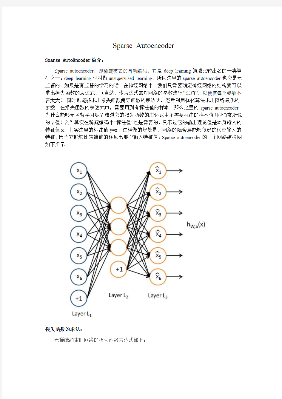
S parse autoencoder，即稀疏模式的自动编码。它是deep learning领域比较出名的一类算法之一。deep learning也叫做unsupervised learning，所以这里的sparse autoencoder也应是无监督的。如果是有监督的学习的话，在神经网络中，我们只需要确定神经网络的结构就可以求出损失函数的表达式了（当然，该表达式需对网络的参数进行”惩罚”，以便使每个参数不要太大）,同时也能够求出损失函数偏导函数的表达式，然后利用优化算法求出网络最优的参数。在损失函数的表达式中，需要用到有标注值的样本。那么这里的sparse autoencoder 为什么能够无监督学习呢？难道它的损失函数的表达式中不需要标注的样本值（即通常所说的y值）么？其实在稀疏编码中”标注值”也是需要的，只不过它的输出理论值是本身输入的特征值x，其实这里的标注值y=x。这样做的好处是，网络的隐含层能够很好的代替输入的特征，因为它能够比较准确的还原出那些输入特征值。Sparse autoencoder的一个网络结构图如下所示：

损失函数的求法：

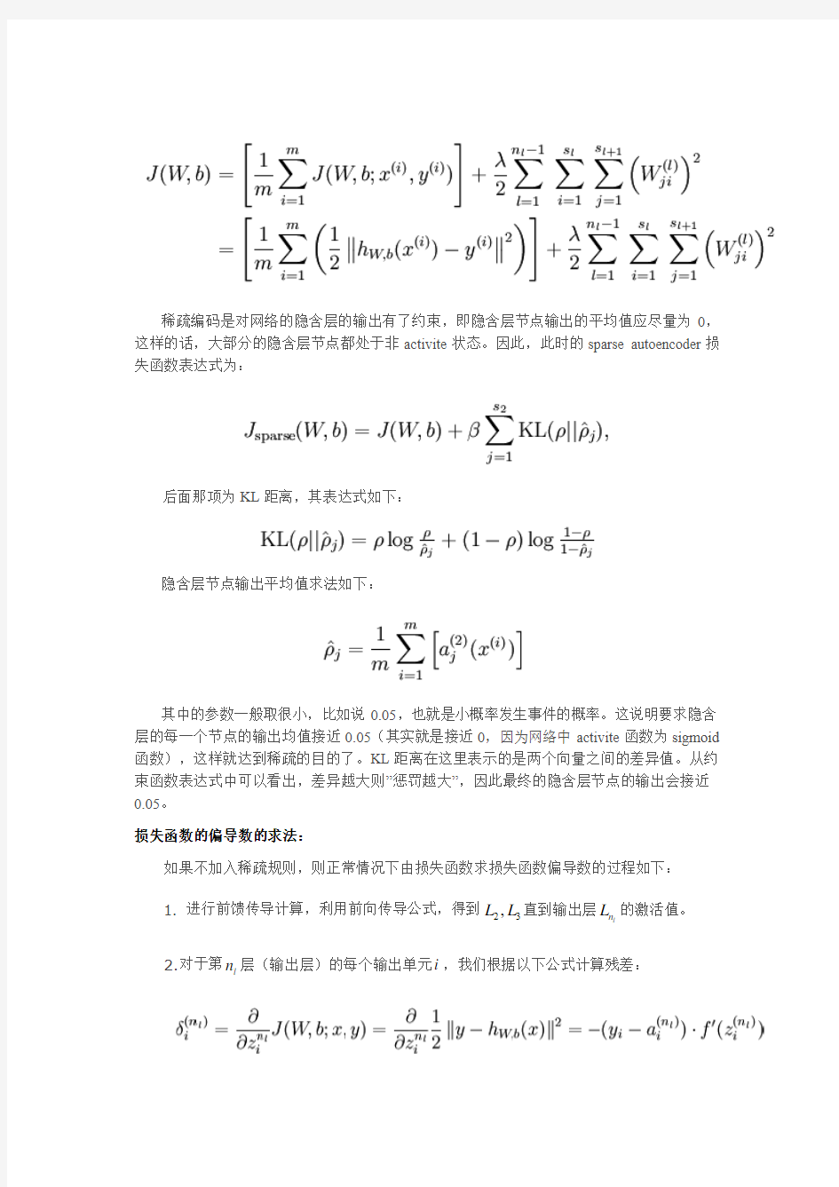
无稀疏约束时网络的损失函数表达式如下：

稀疏编码是对网络的隐含层的输出有了约束，即隐含层节点输出的平均值应尽量为0，这样的话，大部分的隐含层节点都处于非activite 状态。因此，此时的sparse autoencoder 损失函数表达式为：

后面那项为KL 距离，其表达式如下：

隐含层节点输出平均值求法如下：

其中的参数一般取很小，比如说0.05，也就是小概率发生事件的概率。这说明要求隐含层的每一个节点的输出均值接近0.05（其实就是接近0，因为网络中activite 函数为sigmoid 函数），这样就达到稀疏的目的了。KL 距离在这里表示的是两个向量之间的差异值。从约束函数表达式中可以看出，差异越大则”惩罚越大”，因此最终的隐含层节点的输出会接近0.05。

损失函数的偏导数的求法：

如果不加入稀疏规则，则正常情况下由损失函数求损失函数偏导数的过程如下：

1. 进行前馈传导计算，利用前向传导公式，得到23,L L 直到输出层l n L 的激活值。

2.对于第l n 层（输出层）的每个输出单元i ，我们根据以下公式计算残差：

3.对1,2,...,2l l l n n =--的各个层，第l 层的第i 个节点的残差计算方法如下：

4.计算我们需要的偏导数，计算方法如下：

而加入了稀疏性后，神经元节点的误差表达式由公式：

变成公式：

梯度下降法求解：

有了损失函数及其偏导数后就可以采用梯度下降法来求网络最优化的参数了，整个流程如下所示：

1.对于所有l ，令:0l

W ?= , （设置为全零矩阵或全零向量）

2. 对于到，

a. 使用反向传播算法计算和。

b. 计算。

c. 计算。

3. 更新权重参数：

从上面的公式可以看出，损失函数的偏导其实是个累加过程，每来一个样本数据就累加一次。这是因为损失函数本身就是由每个训练样本的损失叠加而成的，而按照加法的求导法则，损失函数的偏导也应该是由各个训练样本所损失的偏导叠加而成。从这里可以看出，训练样本输入网络的顺序并不重要，因为每个训练样本所进行的操作是等价的，后面样本的输入所产生的结果并不依靠前一次输入结果（只是简单的累加而已，而这里的累加是顺序无关的）。

2019年托福高频词汇表：sparse什么意思(附翻译及例句).doc

2019 年托福高频词汇表： sparse什么意思(附翻译及例句 ) sparse 英[sp ɑ：s]美[spɑ：rs] adj. 稀疏的 ; 稀少的稀疏的 ; 稀疏 ; 稀少的 ; 成员稀少疏落词形变化：比较级： sparser比较级：sparsest 派生词： sparsely sparseness sparsity 双语例句 1 . He was a tubby little man in his fifties, with sparse hair. 他 50 来岁，头发稀疏，身材矮胖。来自柯林斯例句 2 . Many slopes are rock fields with sparse vegetation. 很多山坡都是石头地，植被稀疏。来自柯林斯例句 3 . The sparse line of spectators noticed nothing unusual. 那一排稀稀落落的观众没留意到任何不寻常之处。来自柯林斯例句 4 . Traffic was sparse on the highway. 公路上车流稀少。

来自柯林斯例句 5 . the sparse population of the islands 那些岛上零星的人口来自《词典》网络释义 -sparse 1.稀疏的 rebuff 断然拒绝 sparseadj.稀少的;稀疏的spar水疗 2.稀疏 ...索引4.3获取相关矩阵的信息 4.4 改变矩阵的大小和形状 4.5 矩阵元素的移位和排序 4.6 对角矩阵 4.7 空矩阵，标量和向量 4.8 完全矩阵和稀疏 (sparse) 矩阵 4.9 多维数组第 5 章 M文件程序设计第 6 章程序调试和优化第7 章错误处理第8 章数据输入和输出第9 章使用数据工具箱函数第 10 章. 3.稀少的 rebuff 断然拒绝 sparseadj.稀少的;稀疏的spar水疗 4 .成员稀少疏落名字释义—耿希炯...假借为“稀”。稀少〖rare;scarce〗稀疏,成员稀少疏落。同“稀”〖声〖 silent〗. ; 罕见 sparse 〗寂静无相关词条 -sparse rearing 1.薄饲

Sparse Feature Learning for Deep Belief Networks

Sparse Feature Learning for Deep Belief Networks Marc’Aurelio Ranzato1Y-Lan Boureau2,1Yann LeCun1 1Courant Institute of Mathematical Sciences,New York University 2INRIA Rocquencourt {ranzato,ylan,yann@https://www.360docs.net/doc/5d17583440.html,} Abstract Unsupervised learning algorithms aim to discover the structure hidden in the data, and to learn representations that are more suitable as input to a supervised machine than the raw input.Many unsupervised methods are based on reconstructing the input from the representation,while constraining the representation to have cer- tain desirable properties(e.g.low dimension,sparsity,etc).Others are based on approximating density by stochastically reconstructing the input from the repre- sentation.We describe a novel and ef?cient algorithm to learn sparse represen- tations,and compare it theoretically and experimentally with a similar machine trained probabilistically,namely a Restricted Boltzmann Machine.We propose a simple criterion to compare and select different unsupervised machines based on the trade-off between the reconstruction error and the information content of the representation.We demonstrate this method by extracting features from a dataset of handwritten numerals,and from a dataset of natural image patches.We show that by stacking multiple levels of such machines and by training sequentially, high-order dependencies between the input observed variables can be captured. 1Introduction One of the main purposes of unsupervised learning is to produce good representations for data,that can be used for detection,recognition,prediction,or visualization.Good representations eliminate irrelevant variabilities of the input data,while preserving the information that is useful for the ul-timate task.One cause for the recent resurgence of interest in unsupervised learning is the ability to produce deep feature hierarchies by stacking unsupervised modules on top of each other,as pro-posed by Hinton et al.[1],Bengio et al.[2]and our group[3,4].The unsupervised module at one level in the hierarchy is fed with the representation vectors produced by the level below.Higher-level representations capture high-level dependencies between input variables,thereby improving the ability of the system to capture underlying regularities in the data.The output of the last layer in the hierarchy can be fed to a conventional supervised classi?er. A natural way to design stackable unsupervised learning systems is the encoder-decoder paradigm[5].An encoder transforms the input into the representation(also known as the code or the feature vector),and a decoder reconstructs the input(perhaps stochastically)from the repre-sentation.PCA,Auto-encoder neural nets,Restricted Boltzmann Machines(RBMs),our previous sparse energy-based model[3],and the model proposed in[6]for noisy overcomplete channels are just examples of this kind of architecture.The encoder/decoder architecture is attractive for two rea-sons:1.after training,computing the code is a very fast process that merely consists in running the input through the encoder;2.reconstructing the input with the decoder provides a way to check that the code has captured the relevant information in the data.Some learning algorithms[7]do not have a decoder and must resort to computationally expensive Markov Chain Monte Carlo(MCMC)sam-pling methods in order to provide reconstructions.Other learning algorithms[8,9]lack an encoder, which makes it necessary to run an expensive optimization algorithm to?nd the code associated with each new input sample.In this paper we will focus only on encoder-decoder architectures.

SPARSE(稀松矩阵求解器)

●SPARSE（稀松矩阵求解器）适合与求解实数对称或非对称矩阵、复数对称与非对称矩阵。仅适用于静力分析、完全法谐响应分析、完全法瞬态分析、子结构分析、PSD谱分析，对线性与非线性计算均有效。特别的，对于常遇到的正定矩阵的非线性中，SPARSE求解器优先推荐。而在网格拓扑结构常发生变化的接触分析中，SUBSTR求解器具有独特的优势。其他典型的应用有：由SHELL单元或者BEAM单元构建的计算模型；由SHELL单元或者BEAM单元或者SOLID单元构建的计算模型。还有多分支的结构，如汽车尾气排放和涡轮叶片由于将计算速度和效用结合较为完美，因此这是一种进行迭代计算很有效的求解器。一般而言，SAPRSE求解器相对于FRONT求解器而言，需要的内存较小，但是跟PCG求解器使用的计算机内存却大致相当。如果内存有限，该求解器在不增加CPU时间和益处内存的情况下，并不能充分工作。稀疏求解法是使用消元为基础的直接求解法，在ANSYS10.0中其为默认求解选项。其可以支持实矩阵与复矩阵、对称与非对称矩阵、拉格朗日乘子。其支持各类分析，病态矩阵也不会造成求解的困难。稀疏矩阵求解器由于需要存储分解后的矩阵因此对于内存要求较高。其具有一定的并行性，可以利用到4-8cpu. 该求解器具有3种求解方式：核内求解，最优核外求解，最小核外求解。强烈推荐使用核内求解，此时基本不需要磁盘的输入与输出，能大幅度提高求解速度；而核外求解会受到磁盘输入/输出速度的影响。对于复矩阵或非对称矩阵一般需要通常求解2倍的内存与计算时间。相关命令： bcsoption,,incoere 运行核内计算 bcsoption,,optimal 最优核外求解 bcsoption,,minimal 最小核外求解（非正式选项） bcsoption,,force,memrory_size 指定ANSYS使用内存大小 /config,nproce,CPU_number 指定使用cpu的数目 ●FRONT（波前求解器）程序通过三角化消去所有可以由其他自由度表达的自由度，知道最终形成三角矩阵，求解器在三角化过程中保留的节点自由度数目称为波前，在所有自由度被处理后波前为0，整个过程中波前的最大值称为最大波前，最大波前越大所需内存越大。整个过程

《Kernel Sparse Representation》中文翻译

Kernel Sparse Representation-Based Classifier 一、问题： 1、针对不同类别的样本相互融合的分布情况，或者不能用线性的方法将它们有效分开的一般分类问题，SRC 失去了分类能力，如何选择一个有效的方法实现有效分类； 2、KSR 虽然是SRC 的非线性扩展，但是它不能使用用于稀疏信号重构的方法，并且在实验中，测试时间较长，如何缩短测试时间； 3、在KSRC 中，我们需要选择一个参数内核，例如一个RBF 内核，则必须选择有效的方法来确定相应的参数，使得效果优于SRC 的分类效果。二、解决方法：为了解决以上的问题，在SRC 的基础上，文章引入了核函数。核函数定义为： 1212(,)()()T k x x x x φφ=。最常用的核函数分别有：高斯核径向基函数212122(,)()k x x exp x x γ=--，其中0γ>，还有线性核函数：1212(,)T k x x x x =等。文章定义一个训练数据集：()(){}{},|,1,2,...,,1,2,...,m i i i i x y x X R y c i n ∈?∈=，其中，c 是类别的数目，m 是数据输入空间X 的维数，i y 是和i x 相对应的类标。给定一个测试数据集x X ∈，我们的目标是从给定的c 类训练样本中预测出它的实际类标y 。现在定义第j 类训练样本作为矩阵,1,[,...,],1,...,j j m n j j j n X x x R j c ?=∈=的各个列，其中，,j i x 被定义为第j 类样本，j n 是第j 类训练样本的数目。下面定义新的训练样本矩阵来表示所有的样本数据： 12c [,,...,]m n X X X X R ?=∈ 其中，1c j j n n ==∑. 根据映射，将输入空间X （低维空间）的数据映射到核特征空间F （高维空间）中，有：12:()[(),(),...,()]T D x X x x x x F φφφφφ∈→=∈，其中，D m 是核特征空间F 的维度。在SRC 中，测试样本能被在低维输入空间X 中的训练数据线性的表示，同样，我们也能得出在核空间的测试样本有： ()1()n i i i x x φαφφα===∑

Sparse and Low-Rank Matrix Decompositions

Sparse and Low-Rank Matrix Decompositions 摘要：我们考虑如下的基本问题：给定一个由未知稀疏矩阵和未知的低秩矩阵的和的矩阵，能够精确的恢复他们吗？这种恢复的能力有很大的用处在许多领域，一般情况下，这个目标是病态的和NP难的。本文提出了如下的研究：（a）一个新的矩阵不确定性原则；（b）一个简单的基于凸优化的精确分解方法。我们的不确定规则是一个量化的概念，即矩阵不可能稀疏当有漫行列空间时。他决定了什么时候分解问题是病态的，并形成了我们的分解方法和分析基础。我们提出决定条件—在稀疏和低秩元素上—在这种条件下我们的方法可以精确的恢复。 1、引言给定一个由未知稀疏矩阵和未知低秩矩阵加和的矩阵，我们研究如何把矩阵分开为稀疏成分和低秩成分。这样的问题在很多领域得到应用，比如：统计模型选择，机器学习，系统鉴别，计算复杂度理论，及光学等。本文我们提出在何种条件下这个分解问题是适定的，例如，稀疏和低秩成分在根本上是可识别的，目前的凸松弛精确的恢复稀疏和低秩成分。主要结果：令，是一个稀疏矩阵，是一个低秩矩阵。给定矩阵C后，目标是在不知道的稀疏模式和的秩或奇异值的情况下恢复和。在没

有额外条件下这个问题是完全不适定的。在很多条件下，一个特定的解是不存在的；比如说低秩矩阵本身就稀疏，这就使得很难从另一个稀疏矩阵中唯一的区别出来。为了知道何时精确解所示可能的，我们定义了新的秩-稀疏不相关概念，他通过一个不确定原则将矩阵的稀疏模式和矩阵的行或列空间联系到一起。我们的分析是几何形式的，并且从切空间到稀疏和低秩矩阵代数簇扮演了重要的角色。解决这样的分解问题是NP难的。一个合理的首要方法是最小化，满足约束条件A+B=C，式中，作为稀疏和秩的折中。这个问题在解决上是复杂且顽固的；我们提出一个较好的凸优化问题，目标是的凸松弛。我们松弛通过用L1范数来代替他，他表示矩阵A中所有元素绝对值的和。我们松弛通过用核范数来代替他，核范数是矩阵B的奇异值的和。注意到核范数可以被看作是‘L1范数’施加到奇异值上（即矩阵的秩是非零奇异值的个数）。L1范数和核范数是非常好的替代品，并且一些结果给出在一些条件下这些松弛可以恢复稀疏和低秩对象。因此，我们得目的是把C分解为，用如下的凸松弛：

Sparse cooperative Q-learning

Sparse Cooperative Q-learning Jelle R.Kok Nikos Vlassis Informatics Institute,Faculty of Science University of Amsterdam,The Netherlands The full version of this paper appeared in the Proceedings of the21st Interna-tional Conference on Machine Learning in Ban?,Canada,July2004. 1Introduction A multiagent system(MAS)consists of a group of agents that can potentially interact with each other[2].We are interested in fully cooperative multiagent systems,in which the agents have to learn to select individual decisions that result in jointly optimal decisions for the group. In principle,a multiagent system can be regarded as one large single agent,in which each joint action is represented as a single action.The optimal Q-values for the joint actions can then be learned using standard single-agent Q-learning. We will refer to this method as MDP learners.At the other extreme,we have the independent learners(IL)approach in which the agents ignore the actions and rewards of the other agents,and learn their strategies independently.However, the standard convergence proof for Q-learning does not hold in this case,since the transition model depends on the unknown policy of the other learning agents. On the other hand,in many problems agents only have to coordinate with a subset of the agents when in a certain state(e.g.,two cleaning robots cleaning the same room).In this paper we describe a multiagent Q-learning technique,Sparse Cooperative Q-learning,that allows a group of agents to learn how to jointly solve a task given the global coordination requirements of the system. 2Sparse Cooperative Q-Learning In our paper,we?rst examine a compact representation of the state-action space in which the agents learn Q-values based on full joint actions in a prede?ned set of states.In all other(uncoordinated)states,the agents learn based on their individual action.Then we generalize this approach using a context-speci?c coor-dination graph(CG)[1].In a CG each node represents an agent,while an edge de?nes a dependency between two agents.The global coordination problem is now decomposed into a number of local problems that involve fewer agents. In a CG,value rules can be used to specify the dependencies between the agents. These rules de?ne a(local)payo?for a subset of all state and action variables. In our method,the global Q-value for a state equals the sum of the payo?s of all applicable value rules.After every state transition,the payo?of every applicable

Sparse MRI 代码学习笔记

Sparse MRI 代码学习笔记在上周跟老师讨论了关于代码的学习，我又深入的研究了屈小波教授的代码，最近一周我也一直在学习其中的关于Sparse MRI的代码。比较下Michael Lustig 在论文Sparse MRI中提到的每个试验和结果，概括起来，主要分为取样和重建两部分。一．取样取样的方式（即样本的来源）分为仿真模拟取样和标准数据库取样。仿真模拟取样： a.论文中提到的angio image的仿真测试图像是利用random coordinates and orientations 的方式从两个3*3矩阵x=[1,3,6;1,3,6;1,3,6]和y=[1,1,1;,3,3,3;,6,6,6]通过一系列的随机性变换得到的，这种随机性保证了生成图像的普遍性和适用性。 b. noisy_phantom数据库，用于仿真降噪效果图。 c.matlab中使用phantom函数自动产生的大脑仿真图像。 b．标准数据库取样：论文中用到的标准数据库样本包括：calf_data_cs(小腿血管造影图)，brain512(大脑图像)，angio(腿部血管造影图)，brain(大脑图)。取样的方法分为：Full（全取样），LR（欠取样），zf-w/dc（零填充的变密度取样）。 Full取样：使用全1的采样模板与源图像的k-space（原图的fourier变换图）数据作乘。 LR取样：使用部分1的采样模板与源图像的k-space数据作乘。 zf-w/dc取样：根据k-space数据能量主要集中在中心的原理，采用变密度的方式，从中心到边缘采样密度递减，直到采集的样本数足够，这里的变密度取样也包含LR取样，也就是只采样一部分。上图中最后一种采样模式与第三个一样都是变密度采样。

deeplearning论文笔记之(二)sparsefiltering稀疏滤波

Deep Learning论文笔记之（二）Sparse Filtering稀疏滤波 Deep Learning论文笔记之（二）Sparse Filtering稀疏滤波zouxy09@https://www.360docs.net/doc/5d17583440.html,https://www.360docs.net/doc/5d17583440.html,/zouxy09 自己平时看了一些论文，但老感觉看完过后就会慢慢的淡忘，某一天重新拾起来的时候又好像没有看过一样。所以想习惯地把一些感觉有用的论文中的知识点总结整理一下，一方面在整理过程中，自己的理解也会更深，另一方面也方便未来自己的勘察。更好的还可以放到博客上面与大家交流。因为基础有限，所以对论文的一些理解可能不太正确，还望大家不吝指正交流，谢谢。本文的论文来自：Sparse filtering , J. Ngiam, P. Koh, Z. Chen, S. Bhaskar, A.Y. Ng. NIPS2011。在其论文的支撑材料中有相应的Matlab代码，代码很简介。不过我还没读。下面是自己对其中的一些知识点的理解：《Sparse Filtering》本文还是聚焦在非监督学习Unsupervised feature learning算法。因为一般的非监督算法需要调整很多额外的参数hyperparameter。本文提出一个简单的算法：sparse filtering。它只有一个hyperparameter（需要学习的特征数目）需要调整。但它很有效。与其他的特征学习方法不同，sparse filtering并没有明确的构建输入数据的分布的模型。它只优化一个简单的代价函数（L2范数稀疏约束的特征），优化过程可以通过几行简单

的Matlab代码就可以实现。而且，sparse filtering可以轻松有效的处理高维的输入，并能拓展为多层堆叠。 sparse filtering方法的核心思想就是避免对数据分布的显式建模，而是优化特征分布的稀疏性从而得到好的特征表达。一、非监督特征学习一般来说，大部分的特征学习方法都是试图去建模给定训练数据的真实分布。换句话说，特征学习就是学习一个模型，这个模型描述的就是数据真实分布的一种近似。这些方法包括denoising autoencoders，restricted Boltzmann machines (RBMs)，independent component analysis (ICA) 和sparse coding等等。这些方法效果都不错，但烦人的一点就是，他们都需要调节很多参数。比如说学习速率learning rates、动量momentum（好像rbm中需要用到）、稀疏度惩罚系数sparsity penalties和权值衰减系数weight decay等。而这些参数最终的确定需要通过交叉验证获得，本身这样的结构训练起来所用时间就长，这么多参数要用交叉验证来获取时间就更多了。我们花了大力气去调节得到一组好的参数，但是换一个任务，我们又得调节换另一组好的参数，这样就会花了俺们太多的时间了。虽然ICA只需要调节一个参数，但它对于高维输入或者很大的特征集来说，拓展能力较弱。本文中，我们的目标是研究一种简单并且有效的特征学习算法，它只需要最少的参数调节。虽然学习数据分布的模型是可取的，而且效

k-Sparse Autoencoders

a r X i v :1312.5663v 2 [c s .L G ] 22 M a r 2014 Alireza Makhzani makhzani@psi.utoronto.ca Brendan Frey frey@psi.utoronto.ca University of Toronto,10King’s College Rd.Toronto,Ontario M5S 3G4,Canada Abstract Recently,it has been observed that when rep-resentations are learnt in a way that encour-ages sparsity,improved performance is ob-tained on classi?cation tasks.These meth-ods involve combinations of activation func-tions,sampling steps and di?erent kinds of penalties.To investigate the e?ectiveness of sparsity by itself,we propose the “k -sparse autoencoder”,which is an autoen-coder with linear activation function,where in hidden layers only the k highest activities are kept.When applied to the MNIST and NORB datasets,we ?nd that this method achieves better classi?cation results than de-noising autoencoders,networks trained with dropout,and RBMs.k -sparse autoencoders are simple to train and the encoding stage is very fast,making them well-suited to large problem sizes,where conventional sparse cod-ing algorithms cannot be applied. 1.Introduction Sparse feature learning algorithms range from sparse coding approaches (Olshausen &Field ,1997)to training neural networks with sparsity penalties (Nair &Hinton ,2009;Lee et al.,2007).These meth-ods typically comprise two steps:a learning algorithm that produces a dictionary W that sparsely represents the data {x i }N i =1,and an encoding algorithm that,given the dictionary,de?nes a mapping from a new input vector x to a feature vector. A practical problem with sparse coding is that both the dictionary learning and the sparse encoding steps are computationally expensive.Dictionaries are usu-ally learnt o?ine by iteratively recovering sparse codes

matlab中sparse函数

Matlab中Sparse函数函数功能：生成稀疏矩阵。使用方法： (1)S = sparse(A) 将矩阵A转化为稀疏矩阵形式，即矩阵A中任何0元素被去除，非零元素及其下标组成矩阵S。如果A本身是稀疏的，sparse(S)返回S。例如： A = 0 0 0 0 0 0 1 0 0 0 0 0 0 1 0 2 sparse(A) ans = (4,2) 1 (2,3) 1 (4,4) 2 (,)中为元素在矩阵中的位置，后面的数字为其对应的非零值。 (2)S = sparse(i,j,s,m,n,nzmax) 由向量i,j,s生成一个m*n，且最多含有nzmax个元素的稀疏矩阵。例如： sparse([1,2,3,4],[1,2,3,4],[0,0,1,1],5,5,6) ans = (3,3) 1 (4,4) 1 其中i=[1,2,3,4]，对应要形成矩阵的行位置；J=[1,2,3,4]，对应要形成矩阵的列位置； S=[0,0,1,1]，对应要形成矩阵对应位置的值。(注：i和j的位置为一一对应，即(1,1)(2,2)(3,3)(4,4),将s中的值赋给这四个坐标的位置。若i=[2,1,3,4],j=[3,2,4,1]，则形成的坐标为(2,3)(1,2)(3,4),(4,1)，如下例所示。) m=5(>=max(i)),n=5(>=max(j)) (注：m和n的值可以在满足条件的范围内任意选取)，用于限定要形成矩阵的大小； nzmax=6(>=max(i or j))，最多可以有nzmax 各元素，好像没有什么用处。又如： sparse([2,1,3,4],[3,2,4,1],[0,0,1,1],5,5,6) ans = (4,1) 1 (3,4) 1 **一些简写的情况： S = sparse(i,j,s,m,n) 用nzmax = length(s) ； S = sparse(i,j,s) 使m = max(i) 和n = max(j)，在s中零元素被移除前计算最大值，[i j s]中其中一行可能为[m n 0]； S = sparse(m,n) sparse([],[],[],m,n,0)的缩写，生成一个m*n 的所有元素都是0的稀疏矩阵。

Sparse, Sequential Bayesian Geostatistics

Sparse, Sequential Bayesian Geostatistics Dan Cornford, Lehel Csato, Manfred Opper Neural Computing Research Group, School of Engineering and Applied Science, Aston University, Birmingham B4 7ET. Tel. +44 (0)121 359 3611 x4667; Fax. +44 (0)121 333 4586; Email d.cornford@https://www.360docs.net/doc/5d17583440.html, Biography Dr. Dan Cornford is a lecture in Computer Science and works in the Neural Computing Research Group at Aston University. Research interests are in the field of spatial statistics, space-time modelling and data assimilation. Lehel Csato is a post-doc in the same group working on an EPSRC grant (GR/R61857/01) looking at applying sparse sequential Gaussian processes to data assimilation. Manfred Opper is a Reader in the same group, with research interests in statistical physics, sequential learning and Bayesian learning. Introduction A limiting factor to the applicability of geostatistics (random field models / Gaussian processes) is the size of data set that can be analysed. This limit is imposed by computer memory constraints on the storage of the covariance matrix and the computational burden of inverting this matrix. While there are matrix inversion lemmas and computational tricks which can help here, the O(n3) scaling remains. In this paper we propose an alternative approach to geostatistical prediction based on Bayesian learning, that allows a Kalman Filter like sequential algorithm that can also use a sparsity heuristic and learn maximum likelihood estimates of the covariance parameters. This algorithm allows us to apply geostatistics to very large problems, particularly when the resulting process can be represented sparsely. The framework also provides a framework for dealing with non-Gaussian noise models and non-linear observation processes. The Gaussian Process (GP), or random field model defines a probability distribution over the variables of interest, which we call the state variables. For most applications the key advantage of using a GP model is that it allows the user to estimate not just the mean value, but also the uncertainty in the state variables. In the Sparse, Sequential Bayesian (SSB) framework a GP prior distribution is placed over the state variables. The exact form of this prior distribution (that is the choice of the covariance function and the parameters of these) are set by the user, however we have developed an algorithm which allows the computation of the maximum likelihood covariance function parameters as part of the learning process. Theoretical Framework If we denote the state variable as z(x), where x is the spatial index which we drop from now on, the GP prior distribution as p0(z), then learning in GP's (for a single data point) can be viewed as corresponding to the following Bayesian update: P1(z|d) = 1/norm * p(d|z)p0(z) . Thus the updated posterior distribution is equal to a product of an unknown normalising constant, the likelihood, p(d|z), and the prior p0(z). This definition of

SuiteSparse安装笔记

SuiteSparse安装笔记 2016年8月2日 15:23 1、需要支持的数值运算包：BLAS，OpenBLAS（升级编译环境后仍然编译不过，麒麟下能够通过编译），lapack 2、凝思操作系统需要升级或安装的编译环境：cmake，gcc4.9（升级需要gmp、mpc、mpfr、cloog、isl），CUDA，binutils-2.26（OpenBLAS需要） 3、SuiteSparse-4.3.1编译测试（凝思操作系统下，更高版本的需要升级编译环境。）步骤一：安装BLAS包 a、修改make.inc BLASLIB = libblas.a #BLASLIB = blas$(PLAT).a …… #头文件和静态库路径 PROCDIR ?= $(shell pwd | awk -F'/PSA' '{print $$1}') PSAPROCDIR ?= $(PROCDIR)/PSA INSTALL_LIB = $(PSAPROCDIR)/lib INSTALL_INCLUDE = $(PSAPROCDIR)/include b、修改Makefile文件，并执行make或make all all: clean $(BLASLIB) cplib #all: $(BLASLIB) …… cplib: cp $(BLASLIB) $(INSTALL_LIB)/. 步骤二：安装LAPACK包 a、cp make.inc.example make.inc b、修改vi make.inc #OPTS = -O2 -frecursive OPTS = -O3 -funroll-all-loops …… # NOOPT = -O0 -frecursive NOOPT = -O3 -funroll-all-loops …… #头文件和静态库路径 PROCDIR ?= $(shell pwd | awk -F'/PSA' '{print $$1}') PSAPROCDIR ?= $(PROCDIR)/PSA INSTALL_LIB = $(PSAPROCDIR)/lib INSTALL_INCLUDE = $(PSAPROCDIR)/include c、cd /BLAS/SRC修改Makefile，并执行make或make all all: clean $(BLASLIB) #all: $(BLASLIB) d、cd CBLAS，修改Makefile，并执行make或make all #all: all: clean e、回到lapack主目录，修改Makefile #all: lapack_install lib blas_testing lapack_testing all: lapack_install lib blas_testing lapack_testing cplib …… cplib: cp *.a $(INSTALL_LIB)/. 注意：注意编译是否成功，PAS/lib下是否有liblapack.a和libblas.a静态库