Shot-noise statistics in diffusive conductors

a r X i v :c o n d -m a t /0202149v 1 [c o n d -m a t .m e s -h a l l ] 11 F e

b 2002

EPJ manuscript No.

(will be inserted by the editor)

Shot-noise statistics in di?usive conductors

P.-E.Roche 1and B.Dou?c ot 1,2

1Laboratoire de Physique de la Mati`e re Condens′e e,Ecole Normale Sup′e rieure,24rue Lhomond,75231Paris Cedex 05,France 2

Laboratoire de Physique Th′e orique et Hautes Energies,CNRS UMR 7589,Universit Paris VII -Denis Diderot,4place Jussieu,75252Paris Cedex 05,France

Received:date /Revised version:date

Abstract.We study the full probability distribution of the charge transmitted through a mesoscopic di?u-sive conductor during a measurement time ?.We have considered a semi-classical model,with an exclusion principle in a discretized single-particle phase-space.In the large ?limit,numerical simulations show a universal probability distribution which agrees very well with the quantum mechanical prediction of Lee,Levitov and Yakovets [PRB 514079(1995)]for the charge counting statistics.Special attention is given to its third cumulant,including an analysis of ?nite size e?ects and of some experimental constraints for its accurate measurement.

PACS.72.70.+m Electronic transport in condensed matter:Noise processes and phenomena:Electronic transport in mesoscopic or nanoscale materials and structures –73.50.Td Electronic structure and electrical properties of surfaces,interfaces,thin ?lms,and low-dimensional structures:Noise processes and phenomena –71.10.Fd Electronic structure of bulk materials:Lattice fermion models

1Introduction

The electrical current across a conductor results from a ?ow of charge carriers.Their discreetness is responsible for current ?uctuations δi -called shot noise-character-ized by a noise power S I =2

2P.-E.Roche,B.Dou?c ot:Shot-noise statistics in di?usive conductors

2The model

A minimal modeling of out-of-equilibrium semi-classical mesoscopic conductor consists in a1D open system with a?ow and a back-?ow of charges of opposite velocities. This degenerate model can be easily adapted to a one dimensional chain:each site being associated with a back-scattering probability and a Pauli exclusion rule.Such de-generate systems are often considered in the theoretical physics literature as”simple exclusion process”or tra?c models.Indeed some of the analytical results on shot noise power

mentioned previously have been derived with such models[8,22].In order to strictly overlap with these pre-vious studies,we stick with the exact sequence of dynamic rules considered by Liu,Eastman and Yamamoto[22].

The model consists in a chain of N sites.Each site is ei-ther empty,occupied by a right or a left-moving charge or by two charges propagating in opposite directions.During each time step,all charges are shifted to the next site,ac-cording to their direction.After this,each charge is likely to back-scatter with a probability r,provided that the resulting state is empty.The system is maintained out of equilibrium by dissymmetrical boundary conditions:charges are injected at each time step at one end of the chain while both ends act as perfect absorber for charges incoming from the chain.

For the model parameters considered in this paper, over108samples are sometimes required for the statistics to converge up to the desired accuracy.In practice,the nu-merical simulation could still be performed on a desktop computer thanks to a code which core is restricted to low level-processor-instructions.Basically,each con?guration of the chain occupation can be coded by the binary rep-resentation of two integers,one for each charge direction. Each time step is a combination of a register shift(right or left),a bit increment to account for the charge injec-tion at the boundary,and a bit-to-bit comparison of the two integers to check for the scattering which are compat-ible with the Pauli exclusion principle.The e?ectiveness of scattering is set by precomputed series of random bits, refreshed when necessary.A special attention was dedi-cated to the validation of the random numbers algorithm. In addition to this direct simulation,two semi-analytical methods provided a cross validation of the results up to N=6sites.For longer chains,those methods were either too CPU-time or memory consuming.

3Results

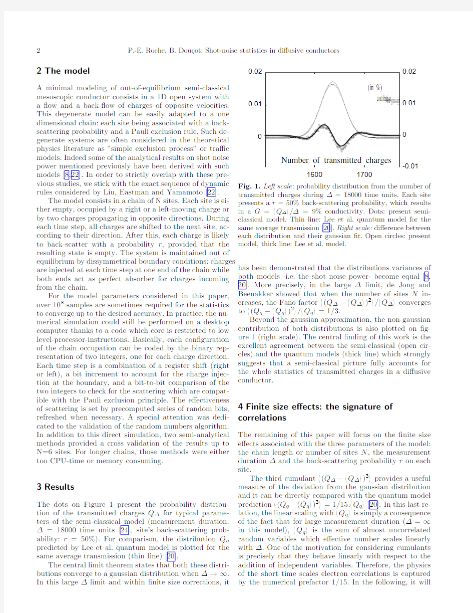
The dots on Figure1present the probability distribu-tion of the transmitted charges Q?for typical parame-ters of the semi-classical model(measurement duration:?=18000time units[24],site’s back-scattering prob-ability:r=50%).For comparison,the distribution Q q predicted by Lee et al.quantum model is plotted for the same average transmission(thin line)[20].

The central limit theorem states that both these distri-butions converge to a gaussian distribution when?→∞. In this large?limit and within?nite size corrections,it

0.01

0.02

-0.01

0.01

0.02

16001700

Fig.1.Left scale:probability distribution from the number of transmitted charges during?=18000time units.Each site presents a r=50%back-scattering probability,which results in a G= Q? /?=9%conductivity.Dots:present semi-classical model.Thin line:Lee et al.quantum model for the same average transmission[20].Right scale:di?erence between each distribution and their gaussian?t.Open circles:present model,thick line:Lee et al.model.

has been demonstrated that the distributions variances of both models-i.e.the shot noise power-become equal[8, 20].More precisely,in the large?limit,de Jong and Beenakker showed that when the number of sites N in-creases,the Fano factor (Q?? Q? )2 / Q? converges to (Q q? Q q )2 / Q q =1/3.

Beyond the gaussian approximation,the non-gaussian contribution of both distributions is also plotted on?g-ure1(right scale).The central?nding of this work is the excellent agreement between the semi-classical(open cir-cles)and the quantum models(thick line)which strongly suggests that a semi-classical picture fully accounts for the whole statistics of transmitted charges in a di?usive conductor.

4Finite size e?ects:the signature of correlations

The remaining of this paper will focus on the?nite size e?ects associated with the three parameters of the model: the chain length or number of sites N,the measurement duration?and the back-scattering probability r on each site.

The third cumulant (Q?? Q? )3 provides a useful measure of the deviation from the gaussian distribution and it can be directly compared with the quantum model prediction (Q q? Q q )3 =1/15. Q q [20].In this last re-lation,the linear scaling with Q q is simply a consequence of the fact that for large measurement duration(?=∞in this model), Q q is the sum of almost uncorrelated random variables which e?ective number scales linearly with?.One of the motivation for considering cumulants is precisely that they behave linearly with respect to the addition of independent variables.Therefore,the physics of the short time scales electron correlations is captured by the numerical prefactor1/15.In the following,it will

P.-E.Roche,B.Dou?c ot:Shot-noise statistics in di?usive conductors

Fig.2.Dependence of the third Fano factor F3= (Q?? Q? )3 / Q? with the measurement duration?for the present model(solid lines)and for the same model without exclusion principle(dashed line).For all curves the back-scattering probability is r=85%.The number of sites per chain is?:2,triangles:4,circles:7.The transient regime evi-dences an anti-correlation time between the charge arrivals.

be useful to call the ratio of the third cumulant by the av-erage transmission the third Fano factor F3,in reference to the usual Fano factor F.

Figure2presents the semiclassical third Fano factor F3= (Q?? Q? )3 / Q? versus the measurement dura-tion?for di?erent combinations of N and r(solid lines). After a transient regime,the signal settles to a constant level.The transient regime duration de?nes a correlation timeτ.Beyond this regime,for?>>τ,the random vari-able Q?scales like?/τas expected and the third Fano factor tends towards a constant value.Note that the mea-surement duration?=18000used in?gure1-to compare Q?and Q q-is validated by a plot similar to?gure2for r=50%.

The simulations show thatτincreases when the chain length is increased as one would expect for a similar model without exclusion principle.In this latter case,we shall show thatτis of the order of the scattering time through the chain.Let us compare further the model with and without exclusion principle.On?gure2,F3versus?is plotted for this second model for the same back-scattering probability and chain lengths(dashed lines).The transient regimes are signi?cantly larger in this second model.In the ?=0limit,F3=1as expected from a Poisson distribu-tion while for large?,F3converges to(1?G).(1?2G) where G= Q? /?is the conductivity.More extensive calculations con?rmed this large?limit,which corre-spond to a binomial distribution.

This result can be understood with the basic sketch of ?gure3.To begin with,the main feature of the model in the absence of exclusion principle is that electrons emitted at di?erent times are completely uncorrelated.The prob-ability distribution of the transmitted charge is therefore completely determined by the probability distribution for a single particle to leave the system on the right,as a function of the time spent inside it.Let us denote byτthe width of this distribution.The left picture on?gure 3illustrates what happens as??τ.Most detected par-ticles have been emitted in region2.For them,the mea-surement window covers the whole span of likely values for their lifetime in the system,before leaving on the right. Region1corresponds to particles emitted early,so they have to spend more time than on average in the system in order to contribute to the signal.Symmetrically,region 3corresponds to particles spending a shorter time than on average in the system.Region1and3have a width of orderτ,whereas region2lasts for a time equivalent to?as??τ.All the particles emitted in region2contribute independently to the signal with the same probability P∞, so the measured charge follows a binomial distribution: P(Q?)?

4P.-E.Roche,B.Dou?c ot:Shot-noise statistics in di?usive conductors

Fig. 3.A simple way to analyze the model in the absence of exclusion principle.Electrons emitted at di?erent times are uncorrelated.They have a ?nite probability to contribute to the signal if their typical arrival time (lying in the tilted band of slope unity and width τ)lies in the measurement window (the horizontal band of width ?).Left large ?limit (??τ).Right:small ?limit (??τ).The picture shows two di?erent measurement windows separated by an interval shorter than τ,which leads to strong anticorrelations between the two

signals.

0.0

0.20

0.40

00.20.40.60.81

F 3 a n d F

Fig.4.Dependence of the Fano F and third Fano factors F 3versus the conductivity G = Q ? /?.The symbols are the data for N=1,2,3,6,10,28sites ;the dotted lines through those symbols are guideline.The thin lines are the dependences for a lumped scatterer predicted by the coherent scattering formalism:(1?G )and (1?G ).(1?2G ).The two plateaux at F =1/3and F 3=1/15are predicted by Lee et al.’s quantum derivation for a di?usive conductor.

Another point of view on these data supports the con-jecture of an asymptotic plateau at 1/15.Figure 5presents the third Fano F 3factor versus the number of sites N for various back-scattering probabilities r .The residual dis-crepancy between the 1/15limit and the N =10data appears as a ?nite size e?ect on N .The inset shows the di?erence between the third Fano factor and 1/15as a function of the number of sites N for r =80%.It is in-teresting to note that the convergence is compatible with a power law with a (?1)exponent,which may be related to long range correlations between charge carriers induced by the exclusion principle.

0.0

F 3

Fig. 5.Dependence of the third Fano F 3factors with the number of sites N .The plateau at F 3=1/15is predicted by Lee et al.Inset :F 3?1/15versus N for r =80%up to N =28.

5Perspective for experiments

To the knowledge of the authors,experiments on the statis-tics of the transmitted charge have never been extended beyond the shot noise power.This may not be surpris-ing since such experiments are di?cult for a fundamental reason:the physical phenomena revealed by higher cu-mulants are related to the correlation time scale τwhile the experimental probes (amperemetre,...)always have a time constant ?such that ??τ.As we recalled ear-lier,in this limit the statistics of transmitted charges are very close to a gaussian and a large number n of statistical samples are required to discern the non-gaussian contri-butions,such as the third Fano factor F 3.In the following,we show that under speci?c experimental conditions,these contributions remain measurable.

We shall ?rst consider the experimental analog of the cumulants (Q ?? Q ? )2 and (Q ?? Q ? )3 from which F and F 3are derived.A central point is the relation be-tween the number of transmitted charges Q ?and the cur-rents i measured by the amperemetre ;our analysis di?ers from a previous one on this point [25].The dynamical re-sponse of the amperemetre is characterized by a cut-o?frequency f B or the corresponding time scale ?=1/f B which can be seen as the duration of the charge counting from which each current output is inferred.Consequently,the relation between Q ?and each current output i should then be:

Q ?～?.i ～i/f B

At this point,two comments are necessary.Firstly,f B should be understood as the e?ective frequency at the amperemetre output,which is set by the whole set-up,including ?lters,cables,...Secondly,in practice,the mea-surement chain is rarely a low pass but rather a bandpass,in order to ?lter out the low frequency noise or as a conse-quence of the typical speci?cations of RF elements.In the following,f B should be understood as the measurement bandwidth rather than the cut-o?frequency.Note that we are implicitly assuming that the shot noise is white,

P.-E.Roche,B.Dou?c ot:Shot-noise statistics in di?usive conductors5 which is reasonable for the experimental conditions con-

sidered below.

Using the previous equation,the Fano factors F and

F3can be written as:

i)3=F3.

(i?

(i?var((i+i N)3)

=i)3/ (i?i2N)3/n

where we used the relation between the variance var of

the statistical estimate of the third cumulant of a gaussian

and its second cumulant.To a reasonable approximation

for our purpose,i)2is the sum of the shot noise2F.e.

(i?i+4k.T/R).f B/2

If S N is the noise power density of i N,we also have:

If the amperemetre output is sampled at a rate f s(over-

sampling being excluded)and if we set S/N=10,the

duration T of the experiment will be:

T=n i+4k.T/R+S N)3

i2.e4.F23

For f B=f s=1GHz,S N=10?24A2/Hz,T=4K, R=50?and

6P.-E.Roche,B.Dou?c ot:Shot-noise statistics in di?usive conductors

point,we may object that a full quantum-mechanical deriva-tion is already available[20].however,this derivation is involving a quenched averaging over the possible impurity con?gurations.For a given mesoscopic sample,this may be justi?ed by an ergodic hypothesis,so that averaging the transmission matrix over a?nite energy window e.V becomes equivalent to impurity averaging.But this may break down for very small systems.Furthermore,semi-classical models are very?exible,since they have been ex-tended to treat interaction e?ects and inelastic processes [16,17,32,33].Again,we believe a detailed analysis of the stationary distribution in con?guration space is required to make further progress.

We want to thank O.Verzelen,T.Jolicoeur,G.Bastard and R.Ferreira for sharing their computing resources.We are also grateful to N.Regnault for some programmer tricks, to H.Willaime and P.Tabeling for technical support with the preliminary experiment mention in[26]and to H. Bouchiat,S.Gu′e ron and B.Reulet for their feed-back. References

1.Blanter Ya.M.and B¨u ttiker M.,Shot noise in mesoscopic conductors,Phys.Rep.336,1(2000).

2.Beenakker C.W.J.and B¨u ttiker M.,Suppression of shot noise in metallic di?usive conductors Phys.Rev.B46,1889 (1992).

3.de Jong M.J.M.and Beenakker C.W.J.,Mesoscopic?uc-tuations in the shot-noise power of metals,Phys.Rev.B46 (20),13400-6(1992).

4.Nazarov Yu.V.,Limits of universality in disordered conduc-tors,Phys.Rev.Lett73(1),134-7(1994).

5.Al’tshuler B.L.,Levitov L.S.and Yakovets A.Yu., Nonequilibrium noise in a mesoscopic conductor:A micro-scopic analysis,Pis’ma Zh.Eksp.Teor.Fiz.59,821(1994). (alternate journal:JETP Lett.59(1994)857)

6.Blanter Ya.M.and B¨u ttiker M.,Shot-noise current-current correlations in multiterminal di?usive conductors,Phys.Rev. B56,2127(1997).

7.Nagaev K.E.,On shot noise in dirty metal contacts,Phys. Lett.A169,103-7(1992).

8.de Jong M.J.M.and Beenakker C.W.J.,Semiclassical theory of shot-noise suppression,Phys.Rev.B51(23),16867-70(1995).

9.Sukhorukov,E.V.and Loss D.,Universality of shot-noise in multiterminal di?usive conductors,Phys.Rev.Lett.80 (22),4959-62(1998).see also Noise in multiterminal di?usive conductors:Universality,nonlocality,and exchange e?ects, Phys.Rev.B59(20),13054-66(1999).

10.Liefrink F.,Dijkhuis J.I.,de Jong M.J.M.,Molenkamp L.W.and van Houten H.,Experimental study of reduced shot noise in a di?usive mesoscopic conductor,Phys.Rev.B49 (19),14066-9(1994).

11.Steinbach A.H.,Martinis J.M.and Devoret M.H.,Obser-vation of hot-electron shot noise in a metallic resistor,Phys. Rev.Lett76,3806(1996).

12.Schoelkopf R.J.,Burke P.J.,Kozhevnikov A.A.,Prober

D.E.and Rooks M.J.,Frequency dependence of shot noise in a di?usive mesoscopic conductor,Phys.Rev.Lett.78(17), 3370-3(1997).13.Henny M.,Oberholzer S.,Strunk C.and Sch¨o nenberger

C.,1/3-shot noise suppression in di?usive nanowires,Phys. Rev.B59(4),2871-80(1999).

https://www.360docs.net/doc/6211011594.html,ndauer,R.,Physica B227,156(1996).

15.de Jong M.J.M.and Beenakker C.W.J.,Semiclassi-cal theory of shot-noise in mesoscopic conductors,Physica A 230,219(1996).

16.Gonz`a lez T.,Gonz`a lez C.,Mateos J.,Pardo D.,Reggiani L.,Bulashenko O.M.and Rubi J.M.,Universality of the 1/3shot-noise suppression factor in nondegenerate di?usive conductors,Phys.Rev.Lett.80(13),2901-4(1998).See also Comment and Reply by Nagaev K.E.,PRL83,1267,(1999), PRL83,1268(1999)

17.Beenakker C.W.J.,Sub-poissonian shot noise in nonde-generate di?usive conductors,Phys.Rev.Lett82(13),2761-3 (1999).

18.Schomerus H.,Mishchenko E.G.,Kinetic theory of shot noise in nondegenerate di?usive conductors,Phys.Rev.B 60(8),5839-50(1999).

19.Levitov L.S.and Lesovik G.B.,Charge distribution in quantum shot noise,JETP Lett.58,230-5(1993).

20.Lee H.,Levitov L.S.and Yakovets A.Yu.,Universal statis-tics of transport in disordered conductors,Phys.Rev.B51 (7),4079-83(1995).

21.Dorokhov O.N.,JETP Lett.36,318(1982).

22.Liu R.C.,Eastman P.,Yamamoto Y.,Inhibition of Elas-tic and inelastic scattering by the Pauli exclusion principle: suppression mechanism for mesoscopic partition noise Solid. State Comm.102,785-9(1997).

23.de Jong M.J.M.,Distribution of transmitted charge trough

a double-barrier junction,Phys.Rev.B54(11),8144-9 (1996).

24.On a64bit processor,if the chain is represented by N=28 bits allocated in the middle of the64bits word,that leaves18 unused bits on each side.Those bits can be used as bu?ers,to di?er and speed up the counting of transmitted and re?ected charges,every18time steps.This very18number explains the somehow odd measurement durations?that are chosen in our computation.

25.Levitov L.S.and Reznikov M.,Electron shot noise beyond the second moment cond-mat/0111057(2001).

26.In this paper,Amperemetre should be understood as a generic name for a detector.For example,we veri?ed ex-perimentally that using of3detectors(voltmeters)con-nected across the conductor under study,we could de-crease the uncertainty on F3below the level expected if we had used one single detector.This performance was possible because the third cumulant R.i)3has been calculated from the output of the3detectors according to R.i1).(R.i2?R.i3),which allows to signi?cantly decrease the e?ect of the voltmeters’voltage noise.For high resistance conductor,a similar trick could decrease the nuisance from the current noise of the detec-tors.Note also that this multi-detectors technique can be generalized for higher moments.

27.In this case f s is the cut-o?frequency of the set-up.

28.Dorfman J.R.,An introduction to chaos in Nonequilibrium statistical mechanics,Cambridge lecture notes in physics14 (1999)chapter13.

29.Kogan Sh.and Shul’man A.Ya.,Zh.Eksp.Teor.Phys.56, 862(1969)[Sov.Phys.JETP29,467(1969)].

P.-E.Roche,B.Dou?c ot:Shot-noise statistics in di?usive conductors7 30.Eyink G.,Lebowitz J.L.and Spchn H.,Hydrodynamics of

Stationary Non-Equilibrium States for Some Stochastic Lat-

tice Gas Models,Communications in Math.Phys.,132,253-

83(1990);Lattice Gas Models in Contact with Stochastic

Reservoirs:Local Equilibrium and Relaxation to the Steady

State,140,119-31(1991).

31.Derrida B.,Lebowitz J.L.and Speer E.R.,Free Energy

Functional for Nonequilibrium Systems:An Exactly Solvable

Case,Phys.Rev.Lett.87,150601(2001).See also Large devi-

ation of the density pro?le in the symmetric simple exclusion

process in cond-mat/0109346

32.Nagaev K.E.,In?uence of electron-electron scattering on

shot noise in di?usive contacts,Phys.Rev.B52(7),4740-3

(1995)

33.Kozub V.I.and Rudin A.M.,Shot noise in mesoscopic

di?usive conductors in the limit of strong electron-electron

scattering,Phys.Rev.B52(11),7853-6(1995).