Insect herbivores drive real time ecological and evolutionary change in plant populaitons

19.B.Wilm,A.Ipenberg,N.D.Hastie,J.B.E.Burch,

D.M.Bader,Development 132,5317(2005).20.B.Zhou et al .,Nature 454,109(2008).

21.B.Lustig et al .,Mol.Cell.Biol.22,1184(2002).

22.S.Hayashi,A.P.McMahon,Dev.Biol.244,305(2002).23.Y.Ruzankina et al .,Cell Stem Cell 1,113(2007).24.N.Barker et al .,Nature 449,1003(2007).25.L.Topol et al .,J.Cell Biol.162,899(2003).26.A.J.Mikels,R.Nusse,PLoS Biol.4,e115(2006).

27.A.Sato,H.Yamamoto,H.Sakane,H.Koyama,A.Kikuchi,

EMBO J.29,41(2010).

28.T.Ishitani et al .,Mol.Cell.Biol.23,131(2003).29.G.J.Hannon,D.Beach,Nature 371,257(1994).

30.H.L.Moses,E.Y.Yang,J.A.Pietenpol,Cell 63,245(1990).31.S.Dennler et al .,EMBO J.17,3091(1998).

32.L.Grumolato et al .,Genes Dev.24,2517(2010).33.M.Yamada et al .,Dev.Dyn.239,941(2010).

34.A.Iavarone,J.Massagué,Nature 387,417(1997).35.N.R.Gough,Sci.Signal.1,eg8(2008).

36.T.P.Yamaguchi,A.Bradley,A.P.McMahon,S.Jones,

Development 126,1211(1999).

37.M.Ito et al .,Nature 447,316(2007).

Acknowledgments:We thank R.Kopan for comments on the manuscript,W.Pu for reagents,and R.Head and

C.Storer for the microarray analysis.This work was funded by the NIH (grant DK90251);the Pew Scholars Program in the Biomedical Sciences;grant 5T35DK074375(Trans-National Institute of Diabetes and Digestive and Kidney Diseases Short-Term Training for Medical Students);the Washington Univ.Digestive Disease Research Core (NIH grant P30-DK52574);and the Intramural Research Program of the NIH,National Cancer Institute,Center for Cancer Research.Microarray data are available on Array Express (accession no.E-MTAB-1175).

Materials transfer agreements will be required for the acquisition of the Wnt5a f/f mice from the National Cancer Institute and the L-WRN cell line from the Washington Univ.Medical School.The data presented in this manuscript are tabulated in the main paper and in the supplementary materials.

Supplementary Materials

https://www.360docs.net/doc/826732560.html,/cgi/content/full/science.1223821/DC1Materials and Methods Figs.S1to S14Tables S1to S3References (38–53)

25April 2012;accepted 21June 2012Published online 6September 2012;10.1126/science.1223821

Insect Herbivores Drive Real-Time Ecological and Evolutionary Change in Plant Populations

Anurag A.Agrawal,1,2*Amy P.Hastings,1Marc T.J.Johnson,3John L.Maron,4Juha-Pekka Salminen 5Insect herbivores are hypothesized to be major factors affecting the ecology and evolution of plants.We tested this prediction by suppressing insects in replicated field populations of a

native plant,Oenothera biennis ,which reduced seed predation,altered interspecific competitive dynamics,and resulted in rapid evolutionary https://www.360docs.net/doc/826732560.html,parative genotyping and phenotyping of nearly 12,000O.biennis individuals revealed that in plots protected from insects,resistance to herbivores declined through time owing to changes in flowering time and lower defensive ellagitannins in fruits,whereas plant competitive ability increased.This independent real-time evolution of plant resistance and competitive ability in the field resulted from the relaxation of direct selective effects of insects on plant defense and through indirect effects due to reduced herbivory on plant competitors.

T

he ubiquitous consumption of plants by insect herbivores represents one of the dominant species interactions on Earth and has been hypothesized to play a strong role in the diversification of plant species and their traits (1–3).The evolution of plant defense has been studied primarily with either a prospective or retrospective approach.Single-generation pro-spective approaches measure contemporary natural selection on resistance traits and make predictions about how those traits should evolve given esti-mates of their heritability (4–6).By contrast,ret-rospective studies compare populations or species that have diverged over time (7–9)and make in-ferences about the processes driving evolutionary change.More generally,temporal studies of natu-ral species interactions that influence evolutionary dynamics remain rare,and few have been exper-imental (9–12).Thus,we lack experimental field studies that quantify how species interactions in-fluence selection on traits and the evolutionary response to this selection.As such,it is not well

established how rapidly plants adapt to selection by herbivores,which traits are most important in the evolution of defense,and whether herbivory drives predictable parallel changes due to selec-tion across populations.

The ecology and evolution of plant-herbivore relationships is,in part,governed by the recipro-cal nature of their interaction and the complex-ity of communities.For example,plant traits and plant community structure are critical for determining insect occurrence and attack rates (1–3).Conversely,insects can directly reduce focal plant abundance (13)or indirectly affect plant abundance through changes in the density of co-occurring competitors (14).Thus,the evolution-ary dynamics of a focal plant species might be influenced through direct selection on resist-ance traits and/or by indirect selection on traits influencing competitive ability (15,16).Despite this likely scenario,our understanding of how species interactions influence the evolution of constituent community members is surprisingly limited (17).

We conducted a field study of the selective impact of insects and the evolutionary response

1

Department of Ecology and Evolutionary Biology,Cornell Uni-versity,Ithaca,NY 14853,USA.2Department of Entomol-ogy,Cornell University,Ithaca,NY 14853,USA.3Department of Biology,University of Toronto at Mississauga,Mississauga,ON L5L 1C6,Canada.4Division of Biological Sciences,University of Montana,Missoula,MT 59812,USA.5Laboratory of Organic Chemistry and Chemical Biology,Department of Chemistry,University of Turku,FI-20014Turku,Finland.

*To whom correspondence should be addressed.E-mail:

agrawal@https://www.360docs.net/doc/826732560.html,

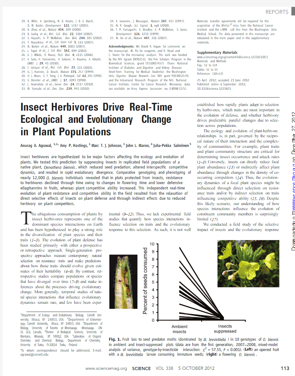
Fig.1.Fruit loss to seed predator moths (dominated by M.brevivittella )in 18genotypes of O.biennis in ambient and insect-suppressed plots (data are from the first generation,2007–2008,mixed-model analysis of variance,genotype-by-insecticide interaction:c 2=57.55,P <0.001).(Left )an opened fruit with a M.brevivittella larvae consuming immature seeds;(right )a flowering O.biennis .

o n D e c e m b e r 27, 2012

w w w .s c i e n c e m a g .o r g D o w n l o a d e d f r o m

to this selection in the native forb common evening primrose,Oenothera biennis(Onagraceae)(18). We established16replicate plots planted with 60individual seedlings of O.biennis,containing equivalent frequencies of18uniquely identi-fied genotypes(19).Half of the plots were treated biweekly during each growing season with esfenvalerate,a nonsystemic insecticide(insect suppression treatment,supplementary text2a); the remaining plots received an equivalent amount of water as a control(ambient insect treat-ment).Because O.biennis is annual or biennial, primarily selfing,and has a genetic system that suppresses recombination and segregation of al-leles,we could track changes in frequencies of each planted genotype within each replicate population over multiple generations(19).Plots were not fur-ther weeded or otherwise manipulated,allowing the natural assembly and early succession of plant species with and without insects(supplementary text2b).We previously summarized our sam-pling methods,the effects of flowering phenology on insect attack,and plant life-history evolution in the ambient insect plots(19).Here,we address the effects of experimental insect suppression on ecological and evolutionary change in O.biennis, including changes in genotypic composition,de-fensive chemistry,competitive ability,and flow-ering time.

Although there were three native species of specialist seed predator moths at our site,fruit loss in O.biennis was dominated by Mompha

brevivittella,which was>5times as abundant as

M.stellella and Schinia florida combined,the

other two common specialists.The18O.biennis

genotypes varied substantially in their resistance

to these seed predators(Fig.1),and insect sup-

pression created an environment with potential-

ly large differences in natural selection.Despite

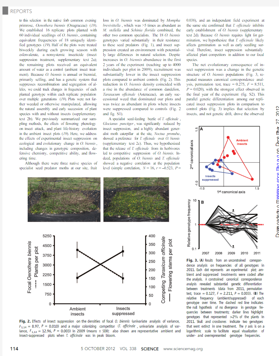
increases in O.biennis abundance in the first

2years of the experiment(reaching up to4000

individuals per plot in2009),recruitment was

substantially lower in the insect suppression

plots compared to ambient controls(Fig.2).This

reduction in O.biennis density coincided with

a rise in the abundance of common dandelion,

Taraxacum officinale(Asteraceae),an early suc-

cessional weed that dominated our plots and

was twice as abundant in plots where insects

were suppressed compared to controls(Fig.2

and fig.S1).

A specialist seed-feeding beetle of T.officinale,

Glocianus punctiger,was significantly reduced by

insect suppression,and a highly abundant gener-

alist moth caterpillar at the site,Noctua pronuba,

showed a preference for T.officinale over O.biennis

(supplementary text2c).Thus,we hypothesized

that the release of T.officinale from its herbivores

led to competitive suppression of O.biennis.In-

deed,populations of O.biennis and T.officinale

showed a negative correlation at the population

level(simple correlation,N=16,r=–0.523,P=

0.038),and an independent field experiment at

the same site confirmed that T.officinale inhibits

early establishment of O.biennis(supplementary

text2d).Because O.biennis requires light for ger-

mination,we hypothesize that T.officinale likely

affects germination as well as early seedling sur-

vival.Therefore,insect suppression substantially

affected plant competitors in addition to our focal

species.

The net evolutionary consequence of in-

sect suppression was a change in the genetic

structure of O.biennis populations(Fig.3,re-

peated measures canonical correspondence anal-

ysis,permutation test,trace=0.275,F=8.511,

P=0.020),with the strongest effect observed in

the final year of the experiment(fig.S2).This

parallel genetic differentiation among our repli-

cated insect suppression plots in comparison to

control plots(Fig.3)implies that selection by

insects,and not genetic drift,drove the

observed

Fig.2.Effects of insect suppression on the densities of focal O.biennis(univariate analysis of variance,

F1,14=8.97,P=0.010)and a major colonizing competitor(T.officinale,univariate analysis of var-

iance,F1,14=12.96,P=0.003)in2009(means T SEM);also shown are representative ambient and

insect-suppressed plots when T.officinale was in peak

bloom.

Fig.3.(A)Results from an unconstrained correspon-

dence analysis on frequencies of all genotypes in

2011.Each dot represents an experimental plot;am-

bient and suppressed treatments were coded after

the analysis.A constrained canonical correspondence

analysis revealed substantial genetic differentiation

between treatments(data from2011,permutation

test,trace=0.127,F=2.211,P=0.003).(B)The

relative frequency(ambient/suppressed)of each

genotype over time.The dashed red line indicates

the null hypothesis of no divergence in genotype fre-

quencies between treatments;darker lines highlight

genotypes that represented>2%of the plants in

2011.Skull and crossbones indicate two genotypes

that went extinct in one treatment.The y axis is on a

logarithmic scale to facilitate equal visualization of

under-and overrepresented genotype frequencies.

o

n

D

e

c

e

m

b

e

r

2

7

,

2

1

2

w

w

w

.

s

c

i

e

n

c

e

m

a

g

.

o

r

g

D

o

w

n

l

o

a

d

e

d

f

r

o

m

genotypic evolution.At the end of the experi-ment,1of the original18genotypes was entire-ly extirpated,and two additional genotypes were represented only in insect suppression plots(Fig.

3).Only six genotypes consistently maintained a frequency of2%or higher within the popula-tions.Three novel genotypes,derived from out-crossing events between known parents,each also reached>2%of the populations in2011(sup-plementary text2e).Thus,across both treatments, nine genotypes dominated all plots(>2%each) at the end of the experiment.Genotypic even-ness was>50%higher in insect suppression plots compared to controls(Smith and Wilson’s even-ness index,E var,univariate analysis of variance, F1,14=15.037,P=0.002),suggesting an erosion of genotypic variance in the presence of insect herbivores.Nonetheless,insect suppression af-fected neither genotypic richness(univariate anal-ysis of variance,F1,14=0.287,P=0.600)nor diversity(Simpson’s index,univariate analysis of variance,F1,14=0.377,P=0.549).

On the basis of annual estimates of genotype frequencies in each plot and genotype-specific means of M.brevivittella attack measured in control plots during2007,we found that experi-mental suppression of insects resulted in evolu-tion of relaxed plant defense(Fig.4).We next determined the evolutionary response of traits re-sponsible for this divergence in resistance.We had previously shown that the extent of early-season flowering(number of open or senesced flowers after50%of the plants had at least a

single open flower)positively correlated with

M.brevivittella attack in2years(19)(i.e.,later-

flowering plants suffered less damage).There

was no difference between treatments in the first

year of our study(2007),as early season flower-

ing was not different among the two treatments

(univariate analysis of variance,F1,14=0.320,

P=0.581);by2010,there was a significant shift

toward earlier flowering in plots with suppressed

insects(univariate analysis of variance,F1,14=

6.105,P=0.027).This effect was even stronger

in2011(Fig.4,univariate analysis of variance,

F1,14=7.025,P=0.019)and was predictable on

the basis of genotype frequencies and genotype-

specific means for early flowering(Fig.4).Thus,

a predicted response to selection was evident in

only three to four generations.We found no dif-

ference in annual versus biennial phenotypes of

O.biennis(repeated measures multivariate anal-

ysis of variance,F1,14=0.935,P=0.350).

O.biennis produces diverse hydrolyzable tan-

nins,including the largest ellagitannins known

from any plant species(20),and these com-

pounds have very high oxidative capacity,nega-

tively affecting insect herbivores(21).One trimer,

oenothein A(fig.S3),was the dominant ellagitan-

nin in O.biennis fruits(up to7.8%dry mass).We

previously showed that oenothein A is favored

by natural selection in O.biennis leaves(6),and

its production in fruits was negatively geneti-

cally correlated with M.brevivittella attack in

the current study(simple correlation,N=17,r=

–0.491,P=0.045)(supplementary text2f),im-

plicating a role of this compound in defense.

Despite a genetic correlation between foliar and

fruit ellagitannin chemistry(simple correlation,

N=18,r=0.848,P<0.001),only fruit chem-

istry significantly diverged in our experimental

plots(Fig.4),suggesting that selection was stron-

gest for defense against flower-and fruit-feeding

herbivores like M.brevivittella.A negative genetic

correlation between early-season flowering and

the production of oenothein A in fruits(simple

correlation,N=23,r=–0.67,P<0.001)is con-

sistent with the rapid and joint evolution of these

traits(i.e.,early flowering with low oenothein A

in insect-suppressed plots)(Fig.4).

Given that insect suppression not only affected

herbivory on O.biennis,but also resulted in stron-

ger plant competition through larger T.officinale

populations,we hypothesized that O.biennis

would evolve greater competitive ability in the

absence of insects.We measured the relative com-

petition index(RCI)in total above-and below-

ground biomass of different genotypes in an

independent experiment(fig.S4).We then used

these genotype-specific values of competitive

ability to determine if the competitive phenotypes

diverged between control and insect-suppressed

plots.Insect suppression resulted in the evolution

of enhanced competitive ability relative to am-

bient insect plots(Fig.4),and because this effect

was not genetically correlated with

early-season

Fig.4.Phenotypic evolution in O.biennis plots.(A)In the presence of seed

predator insects,higher plant resistance evolved[estimated by multiplying

genotype-specific means measured in control(ambient insect)plots by genotype

frequencies in each plot](repeated measures multivariate analysis of variance,

F1,14=6.322,P=0.025),and this effect did not vary over time(time-by-

treatment interaction,repeated measures multivariate analysis of variance,

F3,12=1.459,P=0.275).(B)Earlier flowering was observed in the insect

suppression plots(univariate analysis of variance,F1,14=7.025,P=0.019).

We confirmed that this was an evolutionary response by multiplying genotype-

specific means by genotype frequencies(univariate analysis of variance,F1,14=

4.530,P=0.050);the former field assessment includes the possible effects of

phenotypic plasticity,whereas the latter is based on genotypic values.(C)Leaf

defensive chemistry did not diverge(univariate analysis of variance,F1,14=

1.716,P=0.211)but fruit chemistry changed(univariate analysis of variance,

F1,14=8.917,P=0.010)as predicted by genotypic means and genotype

frequencies.(D)Competitive ability of O.biennis when grown with T.officinale;

plants in the insect-suppressed plots evolved a greater ability to maintain above-

and belowground biomass(relative competition index)when grown with a com-

petitor than when grown alone(repeated measures multivariate analysis of

variance,F1,14=5.189,P=0.038);this effect did not vary over time(repeated

measures multivariate analysis of variance,time-by-treatment interaction(F3,12=

0.072,P=0.974).All panels show means T SEM;ns,not significant.

o

n

D

e

c

e

m

b

e

r

2

7

,

2

1

2

w

w

w

.

s

c

i

e

n

c

e

m

a

g

.

o

r

g

D

o

w

n

l

o

a

d

e

d

f

r

o

m

flowering(simple correlation,N=23,r=–0.157, P=0.474),the production of oenothein A(sim-ple correlation,N=23,r=0.035,P=0.871), or resistance to M.brevivittella(simple correla-tion,N=17,r=–0.255,P=0.241),responses to natural selection were unconstrained by genet-ic correlations.The evolution of increased suscep-tibility to herbivores and enhanced competitive ability was jointly favored by the suppression of insects.

Concurrent evolution of herbivore resistance and competitive ability was only partially predict-able from annual measures of natural selection. We correlated trait values against lifetime seed production in each year,hypothesizing that we would observe divergent slopes concordant with the divergent evolutionary change that we ob-served between our two treatments.Although we found significantly divergent natural selection between ambient and insect suppression plots for the two resistance traits,this effect was ob-served in only1of4years(fig.S5).Nonetheless, when differences in natural selection were ob-served,they were in the predicted direction on the basis of the observed evolutionary change (table S1).Thus,annual measures of natural selec-tion predicted from fecundity were not strong predictors of evolutionary change,which suggests that selection on other components of fitness con-tribute to observed evolutionary responses(19).

Our study provides definitive evidence for the rapid evolution of insect-mediated plant resist-ance traits in real time,supporting current interest in reciprocal feedbacks between evolutionary change and ecological dynamics(17,19,22,23). We highlight how biotic environmental factors simultaneously alter ecological and evolutionary dynamics.Specifically,our finding that multiple herbivores attacking co-occurring host plants can

alter competitive interactions is likely quite gen-

eral in natural ecosystems(14,24,25),and the

rapid evolutionary responses observed confirm

predicted interactive effects of herbivory and com-

petition on plant evolution(15,16).Given that

O.biennis is a poor competitor,we predict that

evolutionary shifts in resistance and competitive

ability allow this species to persist for longer pe-

riods of time during succession.

References and Notes

1.P.R.Ehrlich,P.H.Raven,Evolution18,586(1964).

2.G.S.Fraenkel,Science129,1466(1959).

3.D.J.Futuyma,A.A.Agrawal,Proc.Natl.Acad.Sci.U.S.A.

106,18054(2009).

4.J.Fornoni,P.L.Valverde,J.Nú?ez-Farfán,Evolution58,

1696(2004).

5.R.Mauricio,M.D.Rausher,Evolution51,1435(1997).

6.M.T.J.Johnson,A.A.Agrawal,J.L.Maron,J.P.Salminen,

J.Evol.Biol.22,1295(2009).

7.R.F.Bode,A.Kessler,J.Ecol.100,795(2012).

8.G.A.Desurmont,M.J.Donoghue,W.L.Clement,

A.A.Agrawal,Proc.Natl.Acad.Sci.U.S.A.108,7070

(2011).

9.A.R.Zangerl,M.R.Berenbaum,Proc.Natl.Acad.Sci.U.S.A.

102,15529(2005).

10.P.H.Thrall,J.J.Burdon,Science299,1735(2003).

11.P.R.Grant,B.R.Grant,Science296,707(2002).

12.D.A.Reznick,H.Bryga,J.A.Endler,Nature346,357

(1990).

13.J.L.Maron,E.Crone,Proc.Biol.Sci.273,2575(2006).

14.W.P.Carson,R.B.Root,Ecol.Monogr.70,73

(2000).

15.A.A.Agrawal,https://www.360docs.net/doc/826732560.html,u,P.A.Hamb?ck,Q.Rev.Biol.81,

349(2006).

16.M.Uriarte,C.D.Canham,R.B.Root,Ecology83,2649

(2002).

17.T.W.Schoener,Science331,426(2011).

18.Materials and methods are available as supplementary

materials on Science Online.

19.A.A.Agrawal,M.T.J.Johnson,A.P.Hastings,J.L.Maron,

Am.Nat.10.1086/666727(2012);https://www.360docs.net/doc/826732560.html,/stable/

10.1086/666727.

20.M.Karonen,J.Parker,A.Agrawal,J.P.Salminen,Rapid

Commun.Mass Spectrom.24,3151(2010).

21.R.V.Barbehenn,C.P.Jones,A.E.Hagerman,M.Karonen,

J.P.Salminen,J.Chem.Ecol.32,2253(2006).

22.N.G.Hairston Jr.,S.P.Ellner,M.A.Geber,T.Yoshida,

J.A.Fox,Ecol.Lett.8,1114(2005).

23.M.T.J.Johnson,M.Vellend,J.R.Stinchcombe,Philos.Trans.

R.Soc.Lond.B Biol.Sci.364,1593(2009).

24.J.Lubchenco,S.D.Gaines,Annu.Rev.Ecol.Syst.12,405

(1981).

25.A.A.Agrawal,Ecology85,2118(2004).

Acknowledgments:We thank A.Alfano,F.Chen,S.Cook-Patton,

P.Cooper,T.Dodge,N.Durfee,A.Erwin,M.Falise,J.Goldstein,

E.Kearney,A.Knight,S.McArt,J.Peters,S.Rasmann,A.Smith,

T.Ramsey,E.Reyes,M.Weber,and E.Woods for help with

field work and discussion;T.Zhao,J.Yi,and A.Koivuniemi for

assistance with chemical analyses;and J.Good,N.Hairston,

S.McArt,T.Züst,and the Plant Interactions Group at Cornell

University for comments.Molecular work for this study was

conducted in the Evolutionary Genetics Core Facility at Cornell

University with support from V.Askinazi,S.Bogdanowicz,

R.Harrison,https://www.360docs.net/doc/826732560.html,rson,and E.Reyes.Chemical analyses on an

ultraperformance liquid chromatography–mass spectrometry

system were made possible by a Strategic Research Grant of

University of Turku.This study was primarily supported by a

U.S.NSF grant(EAGER DEB-0950231),and for this we thank

L.Gough.M.T.J.J.was supported by the Natural Sciences and

Engineering Research Council of Canada,the Government

of Ontario,and a Connaught Early Researcher Award;

J.L.M.was supported by NSF grants DEB0614406and

DEB-0915409;J.-P.S was supported by the Academy of Finland

(grant258992).Data sets for genotype frequencies described

in this paper are available in the DRYAD data repository

under https://www.360docs.net/doc/826732560.html,/10.5061/dryad.6331s.This paper is

dedicated to Paul Feeny and Dick Root.

Supplementary Materials

https://www.360docs.net/doc/826732560.html,/cgi/content/full/338/6103/113/DC1

Materials and Methods

Supplementary Text

Figs.S1to S5

Table S1

References(26–32)

12June2012;accepted13August2012

10.1126/science.1225977

Natural Enemies Drive Geographic Variation in Plant Defenses

Tobias Züst,1*?Christian Heichinger,2Ueli Grossniklaus,2Richard Harrington,3 Daniel J.Kliebenstein,4,5Lindsay A.Turnbull1

Plants defend themselves against attack by natural enemies,and these defenses vary widely across populations.However,whether communities of natural enemies are

a sufficiently potent force to maintain polymorphisms in defensive traits is largely unknown.Here,we exploit the genetic resources of Arabidopsis thaliana,

coupled with39years of field data on aphid abundance,to(i)demonstrate that geographic patterns in a polymorphic defense locus(GS-ELONG)are strongly

correlated with changes in the relative abundance of two specialist aphids;and(ii) demonstrate differential selection by the two aphids on GS-ELONG,using a multigeneration selection experiment.We thereby show a causal link between variation

in abundance of the two specialist aphids and the geographic pattern at GS-ELONG,which highlights the potency of natural enemies as selective forces.

I ntraspecific genetic variation is essential in

enabling species to respond rapidly to evolu-tionary challenges such as changing environ-mental conditions(1)or the emergence of novel

pests and pathogens(2).This diversity often re-

flects the balance between the strength of local

selection and the current and historical levels of

population substructure and gene flow(3,4).

Geographic analyses of genetic variation in

several plant species have revealed clear genetic

signals of local adaptation(5),caused by differ-

ences in the selective regime among locations.

These analyses are further supported by reciprocal

transplant experiments,in which home genotypes

generally outperform those transplanted from

other populations(6,7).Although the drivers of

local adaptation often remain unidentified,there

1Institute of Evolutionary Biology and Environmental Studies

and Zürich-Basel Plant Science Center,University of Zürich,

Zürich CH-8057,Switzerland.2Institute of Plant Biology and

Zürich-Basel Plant Science Center,University of Zürich,Zürich

CH-8008,Switzerland.3Rothamsted Insect Survey,AgroEcol-

ogy Department,Rothamsted Research,Harpenden AL52JQ,

UK.4Department of Plant Sciences,University of California at

Davis,Davis,CA95616,USA.5DynaMo Center of Excellence,

Department of Plant Biology and Biotechnology,University of

Copenhagen,Copenhagen DK-1871,Denmark.

*To whom correspondence should be addressed.E-mail:

tobias.zuest@https://www.360docs.net/doc/826732560.html,

?Present address:Department of Ecology and Evolutionary

Biology,Cornell University,Ithaca,NY14853,USA.

o

n

D

e

c

e

m

b

e

r

2

7

,

2

1

2

w

w

w

.

s

c

i

e

n

c

e

m

a

g

.

o

r

g

D

o

w

n

l

o

a

d

e

d

f

r

o

m