大涡模拟的FLUENT算例2D

Tutorial:Modeling Aeroacoustics for a Helmholtz Resonator Using the Direct Method(CAA)

Introduction

The purpose of this tutorial is to provide guidelines and recommendations for the basic setup and solution procedure for a typical aeroacoustic application using computational aeroacoustic(CAA)method.

In this tutorial you will learn how to:

?Model a Helmholtz resonator.

?Use the transient k-epsilon model and the large eddy simulation(LES)model for

aeroacoustic application.

?Set up,run,and perform postprocessing in FLUENT.

Prerequisites

This tutorial assumes that you are familiar with the user interface,basic setup and solution procedures in FLUENT.This tutorial does not cover mechanics of using acoustics model,but focuses on setting up the problem for Helmholtz-Resonator and solving it.It also assumes that you have basic understanding of aeroacoustic physics.

If you have not used FLUENT before,it would be helpful to?rst review FLUENT6.3User’s Guide and FLUENT6.3Tutorial Guide.

Problem Description

A Helmholtz resonator consists of a cavity in a rigid structure that communicates through a

narrow neck or slit to the outside air.The frequency of resonance is determined by the mass of air in the neck resonating in conjunction with the compliance of the air in the cavity.

The physics behind the Helmholtz resonator is similar to wind noise applications like sun roof bu?eting.

We assume that out of the two cavities that are present,smaller one is the resonator.The motion of the?uid takes place because of the inlet velocity of27.78m/s(100km/h).The ?ow separates into a highly unsteady motion from the opening to the small cavity.This unsteady motion leads to a pressure?uctuations.Two monitor points(Point-1and Point-2) act as microphone points to record the generated sound.The acoustic signal is calculated within FLUENT.The?ow exits the domain through the pressure outlet.

Modeling Aeroacoustics for a Helmholtz Resonator Using the Direct Method(CAA) Preparation

1.Copy the?les steady.cas.gz,steady.dat.gz,execute-by-name.scm,stptmstp4.scm,

ti-to-scm-jos.scm and stptmstp.txt into your working directory.

2.Start the2D double precision(2ddp)version of FLUENT.

Setup and Solution

Step1:Grid

1.Read the initial case and data?les for steady-state(steady.cas.gz and steady.dat.gz).

File?→Read?→Case&Data...

Ignore the warning that is displayed in the FLUENT console while reading these?les.

2.Keep default scale for the grid.

Grid?→Scale...

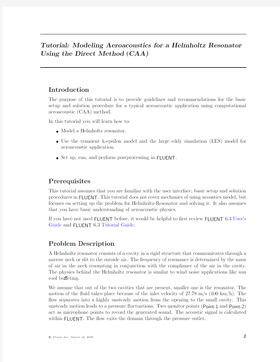
3.Display the grid and observe the locations of the two monitor points,Point-1and

Point-2(Figure1).

Figure1:Graphics Display of the Grid

4.Display and observe the contours of static pressure(Figure2)and velocity magnitude

(Figure3)for the initial steady-state solution.

Display?→Contours..

Modeling Aeroacoustics for a Helmholtz Resonator Using the Direct Method(CAA)

Figure2:Contours of Static Pressure(Steady State)

Figure3:Contours of Velocity Magnitude(Steady State)

Modeling Aeroacoustics for a Helmholtz Resonator Using the Direct Method(CAA) Step2:Models

1.Select unsteady solver.

De?ne?→Models?→Solver...

(a)Select Unsteady in the Time list.

(b)Select2nd-order-implicit in the Unsteady formulation list.

(c)Retain the default settings for other parameters.

(d)Click OK to close the Solver panel.

2.De?ne the viscous model.

De?ne?→Models?→Viscous...

(a)Select Non-Equilibrium Wall Functions in the Near-Wall Treatment list.

(b)Retain the default settigns for other parameters.

(c)Click OK to close the Viscous Model panel.

Near-Wall Treatment predicts good separation and re-attachment points.

Step3:Materials

De?ne?→Materials...

1.Select ideal-gas from the Density drop-down list.

2.Retain the default values for other parameters.

3.Click Change/Create and close the Materials panel.

Ideal gas law is good in predicting the small changes in the pressure.

Step4:Solution

1.Monitor the static pressure on point-1and point-

2.

Solve?→Monitors?→Surface...

(a)Enter2for the Surface Monitors.

(b)Enable Plot and Print options for monitor-1and monitor-2.

(c)Select Time Step from the When list.

(d)Click De?ne...for monitor-1to open De?ne Surface Monitor panel.

Modeling Aeroacoustics for a Helmholtz Resonator Using the Direct Method

(CAA)

i.Select Vertex Average from the Report Type drop-down list.

ii.Select Flow Time from the X Axis drop-down list.

iii.Enter1for Plot Window.

iv.Select point-1from the Surfaces selection list.

(e)Similarly,specify the surface monitor parameters for point-2.

2.Start the calculations using the following settings.

Solve?→Iterate...

(a)Enter3e-04s for Time Step Size.

The expected time step size for this problem is of the size of about1/10th of the

time period.The time period depends on the frequency(f)which is calculated

using the following equation:

f=

c

2π

S

V[L+π

2

.D h

2

]

where,

c=Speed of sound

S=Area of the ori?ce of the resonator

V=Volume of the resonator

L=Length of the connection between the resonator and the free?ow area

D h=Hydraulic diameter of the ori?ce

For this geometry,the estimated frequency is about120Hz.

(b)Enter250for the Number of Time Steps.

(c)Enter50for Max Iterations per Time Step.

(d)Click Apply.

Modeling Aeroacoustics for a Helmholtz Resonator Using the Direct Method(CAA)

(e)Read the scheme?le(stptmstp4.scm).

File?→Read?→Scheme...

This?le activates a alternative convergence criteria.For acoustic simulations

with CAA it is obligatory that the pressure is completely converged at the reciever

position.FLUENT compares the monitor quantities within the last n-de?ned it-

erations to judge if the deviation is smaller than a y-de?ned deviation.

(f)Specify the number of previous iterations from which monitor values of each

quantity used are saved and compared to the current(latest)value(include the

paranthesis):

(set!stptmstp-n5)

(g)Specify the relative(the smaller of two values in any comparison)di?erence

by which any of the older monitor values(for a selected monitor qauntity)may

di?er from the newest value:

(set!stptmstp-maxrelchng1.e-02)

(h)De?ne the execute commands.

Solve?→Execute Commands

i.Enter(stptmstp-resetvalues)for the?rst command and select Time Step

from the drop-down list.

ii.Enter(stptmstp-chckcnvrg"/report/surface-integrals vertex-avg point-1 ()pressure")and select Iteration from the drop-down list.

iii.Click OK.

(i)Click Iterate to start the calculations.

The iterations will take a long time to complete.You can skip this simulation af-

ter few time steps and read the?les(transient.cas.gz and transient.dat.gz)

provided with this tutorial.These?les contain the data for the?ow time of0.22

seconds.As seen in Figures4and5,no pressure?uctuations are present at this

stage.The oscillations of the static pressure at both monitor points has reached

a constant value.

The RANS-simulation is a good starting point for Large Eddy Simulation.If

you choose to use the steady solution as initial condition for LES,use the TUI

command/solve/initialize/init-instantaneous-vel provides to get a more realistic

instantaneous velocity?eld.The usage of LES for acoustic simulations is obliga-

tory.The next two pictures compare the static pressure obtained with RANS and

Large Eddy Simulation for a complete simulation until0.525seconds.Obviously,

the k-epsilon model underpredicts the strong pressure oscillation after reaching

a dynamically steady state(>0.3s)due to its dissipative character.Under-

predicted pressure oscillations lead to underpredicted sound pressure level which

means the acoustic noise is more gentle.

Modeling Aeroacoustics for a Helmholtz Resonator Using the Direct Method(CAA)

Figure4:Convergence History of Static Pressure on Point-1(Transient)

Figure5:Convergence History of Static Pressure on Point-2(Transient)

Modeling Aeroacoustics for a Helmholtz Resonator Using the Direct Method(CAA) Step5:Enable Large Eddy Simulation

1.Enter the following TUI command in the FLUENT console:

(rpsetvar’les-2d?#t)

2.Enable large eddy simulation e?ects.

The k-epsilon model cannot resolve very small pressure?uctuations for aeroacoustic

due to its dissipative https://www.360docs.net/doc/9b5522280.html,e Large Eddy Simulation to overcome this problem.

De?ne?→Models?→Viscous...

(a)Enable Large Eddy Simulation(LES)in the Model list.

(b)Enable WALE in the Subgrid-Scale Model list.

(c)Click OK to close the Viscous Model panel.

An Information panel will appear,warning about bounded central-deferencing be-

ing default for momentum with LES/DES.

Modeling Aeroacoustics for a Helmholtz Resonator Using the Direct Method(CAA)

(d)Click OK to close the Information panel.

3.Retain default discretization schemes and under-relaxation factors.

Solve?→Controls?→Solution...

4.Enable writing of two surface monitors and specify?le names as monitor-les-1.out and

monitor-les-2.out for monitor plots of point-1and point-2respectively.

Solve?→Monitors?→Surface...

To account for stochastic components of the?ow,FLUENT provides two algorithms.

These algorithms model the?uctuating velocity at velocity inlets.With the spec-

tral synthesizer the?uctuating velocity components are computed by synthesizing a

divergence-free velocity-vector?eld from the summation of Fourier harmonics.

5.Enable the spectral synthesizer.

De?ne?→Boundary Conditions...

(a)Select inlet in the Zone list and click Set....

i.Select Spectral Synthesizer from the Fluctuating Velocity Algorithm drop-down

list.

ii.Retain the default values for other parameters.

iii.Click OK to close the Velocity Inlet panel.

(b)Close the Boundary Conditions panel.

Modeling Aeroacoustics for a Helmholtz Resonator Using the Direct Method(CAA) Typically it takes a long time to get a dynamically steady state.Additionally,the

simulated(and recorded for FFT)?ow time depends on the minimum frequency in the

following relationship:

flowtime=

10

minimumfrequency

(1)

The standard transient scheme(iterative time advancement)requires a considerable amount of computaional e?ort due to a large number of outer iterations performed for each time-step.To accelerate the simulation,the NITA(non-iterative time advance-ment)scheme is an alternative.

6.Set the solver parameters.

De?ne?→Models?→Solver...

(a)Enable Non-Iterative Time Advancement in the Transient Controls list.

(b)Click OK to close the Solver panel.

7.Set the solution parameters.

Solve?→Controls?→Solution...

(a)Select Fractional Step from the Pressure-Velocity Coupling drop-down list.

(b)Click OK to close the Solution Controls panel.

8.Disable both the execute commands.

Solve?→Execute Commands...

9.Continue the simulation with the same time step size for1500time steps to get a

dynamically steady solution.

10.Write the case and data?les(unsteady-?nal.cas.gz and unsteady-?nal.dat.gz).

File?→Write?→Case&Data...

Modeling Aeroacoustics for a Helmholtz Resonator Using the Direct Method(CAA)

Figure6:Convergence History of Static Pressure on Point-1(Transient)

Figure7:Convergence History of Static Pressure on Point-2(Transient)

Modeling Aeroacoustics for a Helmholtz Resonator Using the Direct Method(CAA) Step6:Postprocessing

1.Display the contours of static pressure to visualize the eddies near the ori?ce.

2.Enable the acoustics model.

De?ne?→Models?→Acoustics...

(a)Enable Ffowcs-Williams&Hawkings from the Model selection list.

(b)Retain the default value of2e-05Pa for Reference Acoustic Pressure.

To specify a value for the acoustic reference pressure,it is necessary to activate

the acoustic model before starting postprocessing.

(c)Retain default settings for other parameters.

(d)Click OK to accept the settings.

A Warning dialog box appears.This is an informative panel and will not a?ect

the postprocessing results.

(e)Click OK to acknowledge the information and close the Warning panel.

3.Plot the sound pressure level(SPL).

Plot?→FFT...

Modeling Aeroacoustics for a Helmholtz Resonator Using the Direct Method(CAA)

(a)Click Load Input File...button.

(b)Select monitor plot?le for Point-1(monitor-les-1.out).

(c)Click Plot/Modify Input Signal....

i.Select Clip to Range,in the Options list.

ii.Enter0.3for Min and0.5for Max in the X Axis Range group box.

Modeling Aeroacoustics for a Helmholtz Resonator Using the Direct Method(CAA)

iii.Select Hanning in the Window drop-down list.

Hanning shows good performance in frequency resolution.It cuts the time

record more smoothly,eliminating discontinuities that occur when data is

cut o?.

iv.Click Apply/Plot and close the Plot/Modify Input Signal panel.

(d)Select Sound Pressure Level(dB)from the Y Axis Function drop-down list.

(e)Select Frequency(Hz)in the X Axis Function drop-down list.

(f)Click Plot FFT to visualize the frequency distribution at Point-1.

(g)Select Write FFT to File in the Options list.

Note:Plot FFT button will change to Write FFT.

(h)Click Write FFT and specify the name of the FFT?le in the resulting Select File

panel.

(i)Similarly write the FFT?le for monitor plot for point-2(Figure9).

Modeling Aeroacoustics for a Helmholtz Resonator Using the Direct Method(CAA)

Figure8:Spectral Analysis of Convergence History of Static Pressure on Point-1

Figure9:Spectral Analysis of Convergence History of Static Pressure on Point-2

Modeling Aeroacoustics for a Helmholtz Resonator Using the Direct Method(CAA) In Figures8and9,the sound pressure level(SPL)peak occurs at125Hz which is

close to the analytical estimation.Considering that this tutorial uses a slightly large

time step and a2D geometry,the result is?ne.

https://www.360docs.net/doc/9b5522280.html,pare the frequency spectra at point-1and point-2.

Plot?→File...

(a)Click Add...and select two FFT?les(point-1-fft.xy and point-2-fft.xy)

that you have saved in the previous step.

(b)Click Plot to visualize both spectra in the same window(Figure10).

Note that the peak for Point-1is a little higher than for Point-2.This is due to the dissipative behaviour of the sound in the domain.The bigger the distance between the reciever point and the noise source,the bigger is the dissipation of sound.This is the reason,why we use CAA method only for near?eld calculations.

Figure10:Comparison of Frequency Spectra at Point-1and Point-2

A second issue is the dissipation of sound due to the in?uence of the grid size.This applies

especially for which the wave lengths are very short.Thus,a too coarse mesh is not capable of resolving high frequencies correctly.In the present example,the mesh is rather coarse in the far-?eld.Thus,the discrepancy between both spectra is more evident in the high frequency range.

This behaviour can be seen in Figure11.

For high frequencies,the monitor for Point-1generates much fewer noise than monitor for Point-2due to coarse grid resolution.

Modeling Aeroacoustics for a Helmholtz Resonator Using the Direct Method(CAA)

Figure11:Spectral Analysis of Convergence history of Static Pressure The deviation of sound pressure level between the?rst two maximum peaks(50Hz and132 Hz)is quite small.The postprocessing function magnitude in fourier transform panel is similar to the root mean square value(RMS)of the static pressure at these frequencies.

We can use the RMS value to derive the amplitude of the pressure?uctuation which is responsible for the SPL-peak.The resolution of frequency spectra is limited by the temporal discretization.With the temporal discretization,the maximum frequency is

f max=

1

2 t

(2)

This frequency is de?ned as Nyquist frequency.It is the maximum educible frequency.To resolve up to f max the maximum allowable time step size is

f max=

1

2×f max

(3)

Modeling Aeroacoustics for a Helmholtz Resonator Using the Direct Method(CAA)

Figure12:Spectral Analysis of Convergence History of Static Pressure on Point-1

An instability of the?uid motion coupled with an acoustic resonance of the cavity(helmholtz resonator)produces large pressure?uctuations(at132Hz).Compared to this dominant helmholtz resonance the pressure?uctuation at50Hz is quite small.

Modeling Aeroacoustics for a Helmholtz Resonator Using the Direct Method(CAA)

Figure13:Spectral Analysis of Convergence History of Static Pressure on Point-2

Summary

Aeroacoustic simulation of Helmholtz resonator has been performed using k-epsilon model and Large Eddy Simulation model.The advantage of using LES model has been demon-strated.You also learned how the sound dissipation occurs in the domain by monitoring sound pressure level at two di?erent points in the domain.The importance of using CAA method has also been explained.