Learning 3-D Scene Structure from a Single Still Image
Learning3-D Scene Structure from a Single Still Image Ashutosh Saxena,Min Sun and Andrew Y.Ng Computer Science Department,Stanford University,Stanford,CA94305 {asaxena,aliensun,ang}@https://www.360docs.net/doc/9117475878.html,
Abstract
We consider the problem of estimating detailed3-d struc-ture from a single still image of an unstructured environment. Our goal is to create3-d models which are both quantita-tively accurate as well as visually pleasing.
For each small homogeneous patch in the image,we use a Markov Random Field(MRF)to infer a set of“plane param-eters”that capture both the3-d location and3-d orienta-tion of the patch.The MRF,trained via supervised learning, models both image depth cues as well as the relationships between different parts of the image.Inference in our model is tractable,and requires only solving a convex optimiza-tion problem.Other than assuming that the environment is made up of a number of small planes,our model makes no explicit assumptions about the structure of the scene;this enables the algorithm to capture much more detailed3-d structure than does prior art(such as Saxena et al.,2005, Delage et al.,2005,and Hoiem et el.,2005),and also give a much richer experience in the3-d?ythroughs created us-ing image-based rendering,even for scenes with signi?cant non-vertical structure.
Using this approach,we have created qualitatively cor-rect3-d models for64.9%of588images downloaded from the internet,as compared to Hoiem et al.’s performance of 33.1%.Further,our models are quantitatively more accu-rate than either Saxena et al.or Hoiem et al.
1.Introduction
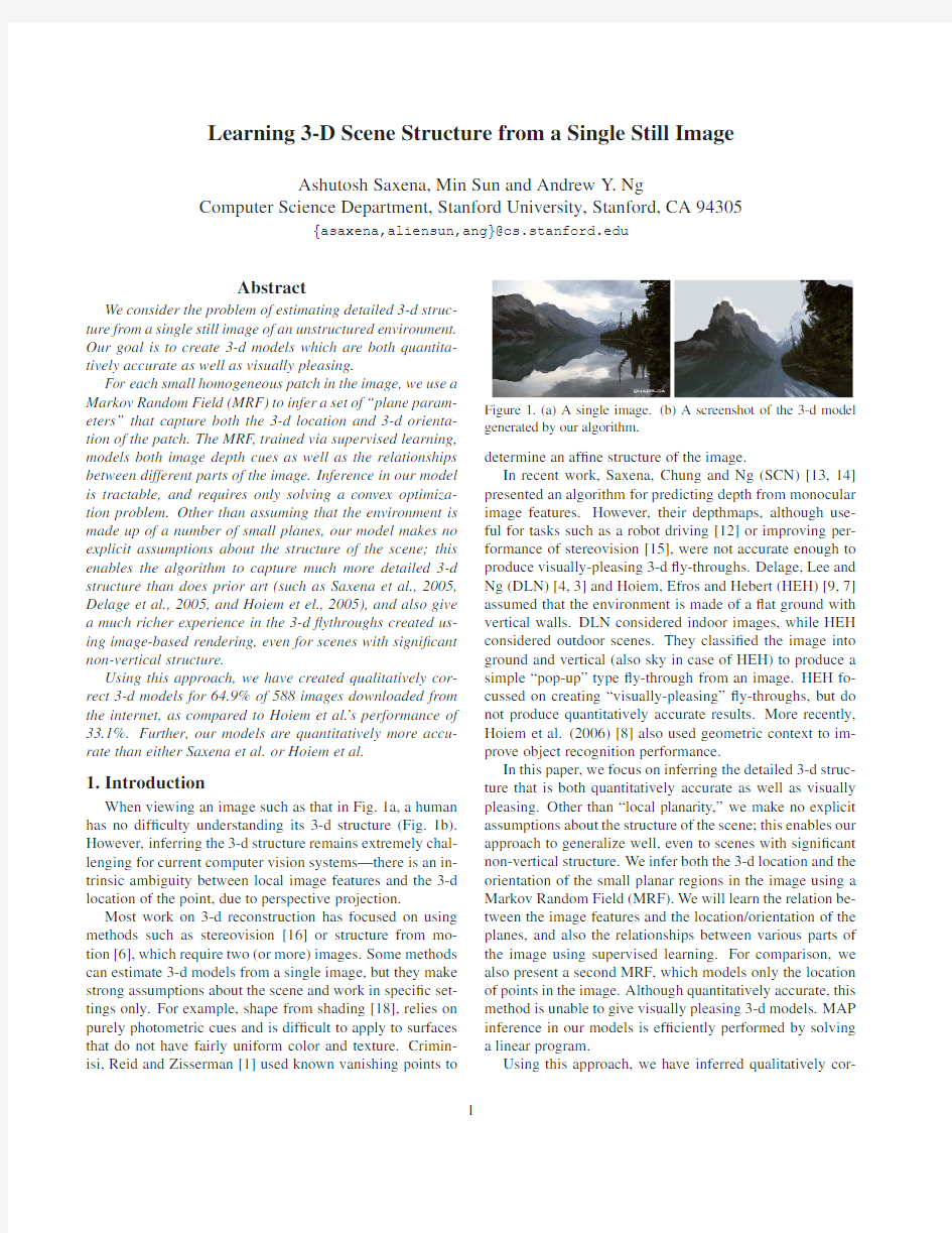
When viewing an image such as that in Fig.1a,a human has no dif?culty understanding its3-d structure(Fig.1b). However,inferring the3-d structure remains extremely chal-lenging for current computer vision systems—there is an in-trinsic ambiguity between local image features and the3-d location of the point,due to perspective projection.
Most work on3-d reconstruction has focused on using methods such as stereovision[16]or structure from mo-tion[6],which require two(or more)images.Some methods can estimate3-d models from a single image,but they make strong assumptions about the scene and work in speci?c set-tings only.For example,shape from shading[18],relies on purely photometric cues and is dif?cult to apply to surfaces that do not have fairly uniform color and texture.Crimin-isi,Reid and Zisserman[1]used known vanishing points
to
Figure1.(a)A single image.(b)A screenshot of the3-d model generated by our algorithm.
determine an af?ne structure of the image.
In recent work,Saxena,Chung and Ng(SCN)[13,14] presented an algorithm for predicting depth from monocular image features.However,their depthmaps,although use-ful for tasks such as a robot driving[12]or improving per-formance of stereovision[15],were not accurate enough to produce visually-pleasing3-d?y-throughs.Delage,Lee and Ng(DLN)[4,3]and Hoiem,Efros and Hebert(HEH)[9,7] assumed that the environment is made of a?at ground with vertical walls.DLN considered indoor images,while HEH considered outdoor scenes.They classi?ed the image into ground and vertical(also sky in case of HEH)to produce a simple“pop-up”type?y-through from an image.HEH fo-cussed on creating“visually-pleasing”?y-throughs,but do not produce quantitatively accurate results.More recently, Hoiem et al.(2006)[8]also used geometric context to im-prove object recognition performance.
In this paper,we focus on inferring the detailed3-d struc-ture that is both quantitatively accurate as well as visually pleasing.Other than“local planarity,”we make no explicit assumptions about the structure of the scene;this enables our approach to generalize well,even to scenes with signi?cant non-vertical structure.We infer both the3-d location and the orientation of the small planar regions in the image using a Markov Random Field(MRF).We will learn the relation be-tween the image features and the location/orientation of the planes,and also the relationships between various parts of the image using supervised learning.For comparison,we also present a second MRF,which models only the location of points in the image.Although quantitatively accurate,this method is unable to give visually pleasing3-d models.MAP inference in our models is ef?ciently performed by solving
a linear program.
Using this approach,we have inferred qualitatively cor-1
rect and visually pleasing3-d models automatically for 64.9%of the588images downloaded from the internet,as compared to HEH performance of33.1%.“Qualitatively correct”is according to a metric that we will de?ne later. We further show that our algorithm predicts quantitatively more accurate depths than both HEH and SCN.
2.Visual Cues for Scene Understanding
Images are the projection of the3-d world to two dimensions—hence the problem of inferring3-d structure from an image is degenerate.An image might represent an in?nite number of3-d models.However,not all the possi-ble3-d structures that an image might represent are valid; and only a few are likely.The environment that we live in is reasonably structured,and hence allows humans to infer3-d structure based on prior experience.
Humans use various monocular cues to infer the3-d structure of the scene.Some of the cues are local proper-ties of the image,such as texture variations and gradients, color,haze,defocus,etc.[13,17].Local image cues alone are usually insuf?cient to infer the3-d structure.The ability of humans to“integrate information”over space,i.e.,under-standing the relation between different parts of the image,is crucial to understanding the3-d structure.[17,chap.11] Both the relation of monocular cues to the3-d structure, as well as relation between various parts of the image is learned from prior experience.Humans remember that a structure of a particular shape is a building,sky is blue,grass is green,trees grow above the ground and have leaves on top of them,and so on.
3.Image Representation
We?rst?nd small homogeneous regions in the image, called“Superpixels,”and use them as our basic unit of rep-resentation.(Fig.6b)Such regions can be reliably found us-ing over-segmentation[5],and represent a coherent region in the image with all the pixels having similar properties.In most images,a superpixel is a small part of a structure,such as part of a wall,and therefore represents a plane.
In our experiments,we use algorithm by[5]to obtain the superpixels.Typically,we over-segment an image into about 2000superpixels,representing regions which have similar color and texture.Our goal is to infer the location and orien-tation of each of these superpixels.
4.Probabilistic Model
It is dif?cult to infer3-d information of a region from local cues alone,(see Section2)and one needs to infer the 3-d information of a region in relation to the3-d information of other region.
In our MRF model,we try to capture the following prop-erties of the images:
?Image Features and depth:The image features of
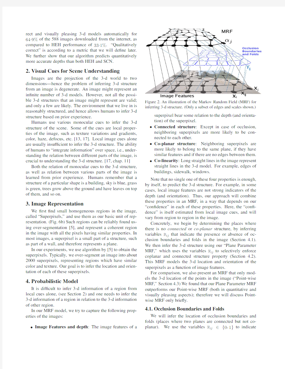
a Figure2.An illustration of the Markov Random Field(MRF)for inferring3-d structure.(Only a subset of edges and scales shown.) superpixel bear some relation to the depth(and orienta-tion)of the superpixel.
?Connected structure:Except in case of occlusion, neighboring superpixels are more likely to be con-nected to each other.
?Co-planar structure:Neighboring superpixels are more likely to belong to the same plane,if they have similar features and if there are no edges between them.?Co-linearity:Long straight lines in the image represent straight lines in the3-d model.For example,edges of buildings,sidewalk,windows.
Note that no single one of these four properties is enough, by itself,to predict the3-d structure.For example,in some cases,local image features are not strong indicators of the depth(and orientation).Thus,our approach will combine these properties in an MRF,in a way that depends on our “con?dence”in each of these properties.Here,the“con?-dence”is itself estimated from local image cues,and will vary from region to region in the image.
Concretely,we begin by determining the places where there is no connected or co-planar structure,by inferring variables y ij that indicate the presence or absence of oc-clusion boundaries and folds in the image(Section4.1). We then infer the3-d structure using our“Plane Parameter MRF,”which uses the variables y ij to selectively enforce coplanar and connected structure property(Section4.2). This MRF models the3-d location and orientation of the superpixels as a function of image features.
For comparison,we also present an MRF that only mod-els the3-d location of the points in the image(“Point-wise MRF,”Section4.3)We found that our Plane Parameter MRF outperforms our Point-wise MRF(both in quantitative and visually pleasing aspects);therefore we will discuss Point-wise MRF only brie?y.
4.1.Occlusion Boundaries and Folds
We will infer the location of occlusion boundaries and folds(places where two planes are connected but not co-planar).We use the variables y ij∈{0,1}to indicate
whether an “edgel”(the edge between two neighboring su-perpixels)is an occlusion boundary/fold or not.The infer-ence of these boundaries is typically not completely accu-rate;therefore we will infer soft values for y ij .More for-mally,for an edgel between two superpixels i and j ,y ij =0indicates an occlusion boundary/fold,and y ij =1indicates none (i.e.,a planar surface).We model y ij using a logis-tic response as P (y ij =1|x ij ;ψ)=1/(1+exp(?ψT x ij ).where,x ij are features of the superpixels i and j (Sec-tion 5.2),and ψare the parameters of the model.During inference (Section 4.2),we will use a mean ?eld-like ap-proximation,where we replace y ij with its mean value under the logistic model.
4.2.Plane Parameter MRF
In this MRF,each node represents a superpixel in the im-age.We assume that the superpixel lies on a plane,and we will infer the location and orientation of that plane.
Representation :We parameterize both the location and ori-entation of the in?nite plane on which the superpixel
lies Figure 3.A 2-d illustration to ex-plain the plane parameter αand
rays R from the camera.
by using plane parame-ters α∈R 3.(Fig.3)(Any point q ∈R 3lying on the plane with param-eters αsatis?es αT q =1.)The value 1/|α|is the
distance from the cam-era center to the closest
point on the plane,and the normal vector ?α=α|α|gives the orientation of the plane.If R i is the unit vector from the camera center to a point i
lying on a plane with parameters α,then d i =1/R T
i αis the distance of point i from the camera center.
Fractional depth error :For 3-d reconstruction,the frac-tional (or relative)error in depths is most meaningful;and is used in structure for motion,stereo reconstruction,etc.[10,16]For ground-truth depth d ,and estimated depth ?d
,fractional error is de?ned as (?d ?d )/d =?d/d ?1.There-fore,we would be penalizing fractional errors in our MRF.Model :To capture the relation between the plane param-eters and the image features,and other properties such as co-planarity,connectedness and co-linearity,we formulate our MRF as
P (α|X,Y,R ;θ)=1Z
i f θ(αi ,X i ,y i ,R i )
i,j
g (αi ,αj ,y ij ,R i ,R j )(1)where,αi is the plane parameter of the superpixel i .For
a total of S i points in the superpixel i ,we use x i,s i to denote the features for point s i in the superpixel i .X i ={x i,s i ∈R 524:s i =1,...,S i }are the features for the superpixel i .(Section 5.1)Similarly,R i ={R i,s i :s i =1,...,S i }is the set of rays for superpixel i
.
Figure 4.An illustration to explain effect of the choice of s i and s j on enforcing the following properties:(a)Partially connected,(b)Fully connected,and (c)Co-planar.
The ?rst term f (.)models the plane parameters as a func-tion of the image features x i,s i .We have R T
i,s i αi
=1/d i,s i
(where R i,s i is the ray that connects the camera to the 3-d lo-cation of point s i ),and if the estimated depth ?d i,s i =x T i,s i
θr ,then the fractional error would be (R T i,s i αi (x T
i,s i θr )?1).Therefore,to minimize the aggregate fractional error over all the points in the superpixel,we model the relation be-tween the plane parameters and the image features as
f θ(αi ,X i ,y i ,R i )=exp ? S i s i =1νi,s i R T i,s i αi (x T i,s i θr )?1 The parameters of this model are θr ∈R 524.We use
different parameters (θr )for each row r in the image,be-cause the images we consider are taken from a horizontally mounted camera,and thus different rows of the image have different statistical properties.E.g.,a blue superpixel might be more likely to be sky if it is in the upper part of im-age,or water if it is in the lower part of the image.Here,y i ={νi,s i :s i =1,...,S i }and the variable νi,s i indicates
the con?dence of the features in predicting the depth ?d i,s i
at point s i .1
If the local image features were not strong enough to predict depth for point s i ,then νi,s i =0turns off the effect of the term R T
i,s i αi (x T
i,s i θr )?1 .
The second term g (.)models the relation between the plane parameters of two superpixels i and j .It uses pairs of points s i and s j to do so:
g (.)=
{s i ,s j }∈N h s i ,s j (.)(2)We will capture co-planarity,connectedness and co-linearity,by different choices of h (.)and {s i ,s j }.
Connected structure :We enforce this constraint by choosing s i and s j to be on the boundary of the superpix-els i and j .As shown in Fig.4b,penalizing the distance between two such points ensures that they remain fully con-nected.Note that in case of occlusion,the variables y ij =0,and hence the two superpixels will not be forced to be con-nected.The relative (fractional)distance between points s i and s j is penalized by
h s i ,s j (αi ,αj ,y ij ,R i ,R j )=exp ?y ij |(R T i,s i αi ?R T j,s j αj )?d |
1The
variable νi,s i is an indicator of how good the image features
are in predicting depth for point s i in superpixel i .We learn νi,s i from the monocular image features,by estimating the expected value of
|d i ?x T i θr |/d i as φT r x i with logistic response,with φr as the parameters
of the model,features x i and d i as ground-truth depths.
In detail,R T i,s
i αi=1/d i,s
i
and R T j,s
j
αj=1/d j,s
j
;there-
fore,the term(R T i,s
i αi?R T j,s
j
αj)?d gives the fractional dis-
tance|(d i,s
i ?d j,s
j
)/
d i,s
i
d j,s
j
|for?d=
d s
i
d s
j
.
Figure5.A2-d illustration to explain the co-planarity term.The distance of the point s j on superpixel j to the plane on which su-
perpixel i lies along the ray R j,s
j”is given by d1?d2.
Co-planarity:We enforce the co-planar structure by choosing a third pair of points s i and s j in the center of each superpixel along with ones on the boundary.(Fig.4c) To enforce co-planarity,we penalize the relative(fractional) distance of point s j from the plane in which superpixel i lies,along the ray R j,s
j
(See Fig.5).
h s
j (αi,αj,y ij,R j,s
j
)=exp
?y ij|(R T j,s
j
αi?R T j,s
j
αj)?d s
j
|
with h s
i ,s j
(.)=h s
i
(.)h s
j
(.).Note that if the two super-
pixels are coplanar,then h s
i ,s j
=1.To enforce co-planarity
between two distant planes that are not connected,we can choose3pairs of points and use the above penalty.
Co-linearity:Finally,we enforce co-linearity constraint using this term,by choosing points along the sides of long straight lines.This also helps to capture relations between regions of the image that are not immediate neighbors. Parameter Learning and MAP Inference:Exact param-eter learning of the model is intractable;therefore,we use Multi-Conditional Learning(MCL)for approximate learn-ing,where we model the probability as a product of multiple conditional likelihoods of individual densities.[11]We esti-mate theθr parameters by maximizing the conditional like-lihood log P(α|X,Y,R;θr)of the training data,which can be written as a Linear Program(LP).
MAP inference of the plane parameters,i.e.,maximiz-ing the conditional likelihood P(α|X,Y,R;θ),is ef?ciently performed by solving a LP.To solve the LP,we implemented an ef?cient method that uses the sparsity in our problem al-lowing inference in a few seconds.
4.3.Point-wise MRF
We present another MRF,in which we use points in the image as basic unit,instead of superpixels;and infer only their3-d location.The nodes in this MRF are a dense grid of points in the image,where the value of each node represents its depth.The depths in this model are in log scale to em-phasize fractional(relative)errors in depth.Unlike SCN’s ?xed rectangular grid,we use a deformable grid,aligned with structures in the image such as lines and corners to im-prove performance.Further,in addition to using the con-nected structure property(as in SCN),our model also cap-tures co-planarity and co-linearity.Finally,we use logis-
tic response to identify occlusion and folds,whereas SCN learned the variances.
In the MRF below,the?rst term f(.)models the relation between depths and the image features as fθ(d i,x i,y i)=
exp
?y i|d i?x T iθr(i)|
.The second term g(.)mod-
els connected structure by penalizing differences in depth of neighboring points as g(d i,d j,y ij,R i,R j)= exp(?y ij|(R i d i?R j d j)|).The third term h(.)depends
on three points i,j and k,and models co-planarity and co-linearity.(Details omitted due to space constraints;see full paper for details.)
P(d|X,Y,R;θ)=
1
Z
i
fθ(d i,x i,y i)
i,j∈N
g(d i,d j,y ij,R i,R j)
i,j,k∈N
h(d i,d j,d k,y ijk,R i,R j,R k)
where,d i∈R is the depth at a point i.x i are the image features at point i.MAP inference of depths,i.e.maxi-mizing log P(d|X,Y,R;θ)is performed by solving a linear program(LP).However,the size of LP in this MRF is larger than in the Plane Parameter MRF.
5.Features
For each superpixel,we compute a battery of features to capture some of the monocular cues discussed in Section2.
We also compute features to predict meaningful boundaries
in the images,such as occlusion.Note that this is in contrast
with some methods that rely on very speci?c features,e.g. computing parallel lines on a plane to determine vanishing points.Relying on a large number of different types of fea-tures helps our algorithm to be more robust and generalize
to images that are very different from the training set.
5.1.Monocular Image Features
For each superpixel at location i,we compute texture-based summary statistic features,and superpixel shape and location based features.2(See Fig.6.)We attempt to cap-
ture more“contextual”information by also including fea-tures from neighboring superpixels(4in our experiments),
and at multiple spatial scales(3in our experiments).(See Fig.6.)The features,therefore,contain information from
a larger portion of the image,and thus are more expressive
2Similar to SCN,we use the output of each of the17(9Laws masks,
2color channels in YCbCr space and6oriented edges)?lters F n(x,y),
n=1,...,17as:E i(n)=
P
(x,y)∈S i
|I(x,y)?F n(x,y)|k,where
k=2,4gives the energy and kurtosis respectively.This gives a total of34 values for each superpixel.We compute features for a superpixel to improve performance over SCN,who computed them for?xed rectangular patches.
Our superpixel shape and location based features included the shape and location based features in Section2.2of[9],and also the eccentricity of the superpixel.
Figure 6.The feature vector for a superpixel,which includes immediate and distant neighbors in multiple scales.(Best viewed in color.)
than just local features.This makes the feature vector x i of a superpixel 524dimensional.
5.2.Features for Boundaries
Another strong cue for 3-d structure perception is bound-ary information.If two neighbor superpixels of an im-age display different features,humans would often perceive them to be parts of different objects;therefore an edge be-tween two superpixels with distinctly different features,is a candidate for a occlusion boundary or a fold.To compute the features x ij between superpixels i and j ,we ?rst generate 14different segmentations for each image for 2different scales for 7different properties:textures,color,and edges.Each element of our 14dimensional feature vector x ij is then an indicator if two superpixels i and j lie in the same segmen-tation.The features x ij are the input to the classi?er for the occlusion boundaries and folds.(see Section 4.1)
6.Incorporating Object Information
In this section,we will discuss how our model can also in-corporate other information that might be available,for ex-ample,from object recognizers.In [8],Hoiem et https://www.360docs.net/doc/9117475878.html,ed knowledge of objects and their location to improve the esti-mate of the horizon.In addition to estimating the horizon,the knowledge of objects and their location in the scene gives strong cues regarding the 3-d structure of the scene.For ex-ample,a person is more likely to be on top of the ground,rather than under it.
Here we give some examples of such constraints,and de-scribe how we can encode them in our MRF:(a)“Object A is on top of object B”
This constraint could be encoded by restricting the points s i ∈R 3on object A to be on top of the points s j ∈R 3on object B,i.e.,s T i ?z ≥s T j ?z
(if ?z denotes the “up”vector).In practice,we actually use a probabilistic version of this constraint.We represent this inequality in plane-parameter
space (s i =R i d i =R i /(αT
i R i )).To penalize the fractional
error ξ= R T i ?z R T j αj ?R T j ?z R i αi ?d
(the constraint corre-sponds to ξ≥0),we choose an MRF potential h s i ,s j (.)=exp (?y ij (ξ+|ξ|)),where y ij represents the uncertainty in the object recognizer output.Note that for y ij →∞(corre-sponding to certainty in the object recognizer),this becomes
a “hard”constraint R T i ?z /(αT i R i )≥R T j ?z /(αT
j R j ).
In fact,we can also encode other similar spatial-relations by choosing the vector ?z appropriately.For example,a con-straint “Object A is in front of Object B”can be encoded by choosing ?z to be the ray from the camera to the object.(b)“Object A is attached to Object B”
For example,if the ground-plane is known from a recog-nizer,then many objects would be more likely to be “at-tached”to the ground plane.We easily encode this by using our connected-structure constraint (Section 4).(c)Known plane orientation
If orientation of a plane is roughly known,e.g.that a person is more likely to be “vertical”,then it can be easily encoded by adding to Eq.1a term f (αi )=exp ?νi |αT i ?z | ;here,νi represents the con?dence,and ?z represents the up vector.We will describe our results using these constraints in Section 7.3.
7.Experiments
7.1.Data collection
We used a custom-built 3-D scanner to collect images and
their corresponding depthmaps using lasers.We collected a total of 534images+depthmaps,with an image resolution of 2272x1704and a depthmap resolution of 55x305;and used 400for training our model.
We tested our model on 134images collected using our 3-d scanner,and also on 588internet images.The images on the internet were collected by issuing keywords on Google image search.To collect data and to perform the evaluation of the algorithms in a completely unbiased manner,a person not associated with the project was asked to collect images of environments (greater than 800x600size).The person chose the following keywords to collect the images:campus,garden,park,house,building,college,university,church,castle,court,square,lake,temple,scene.
7.2.Results and Discussion
We performed an extensive evaluation of our algorithm on 588internet test images,and 134test images collected using the laser scanner.
In Table 1,we compare the following algorithms:
(a)Baseline:Both for depth-MRF (Baseline-1)and plane parameter MRF (Baseline-2).The Baseline MRF is trained
Figure 7.(a)Original Image,(b)Ground truth depthmap,(c)Depth from image features only,(d)Point-wise MRF,(e)Plane parameter MRF.(Best viewed in Color )
Table 1.Results:Quantitative comparison of various methods.
M ETHOD CORRECT %PLANES log 10R EL
(%)CORRECT
SCN NA NA 0.1980.530
HEH 33.1%50.3%0.320 1.423
B ASELINE -10%NA 0.3000.698N O PRIORS 0%NA 0.1700.447
P OINT -WISE MRF 23%NA 0.1490.458
B ASELINE -20%0%0.3340.516
N O PRIORS 0%0%0.2050.392
C O -PLANAR 45.7%57.1%0.1910.373
PP-MRF 64.9%71.2%0.1870.370
without any image features,and thus re?ects a “prior”
depthmap of sorts.
(b)Our Point-wise MRF:with and without constraints (con-nectivity,co-planar and co-linearity).
(c)Our Plane Parameter MRF (PP-MRF):without any con-straint,with co-planar constraint only,and the full model.(d)Saxena et al.(SCN),applicable for quantitative errors.(e)Hoiem et al.(HEH).For fairness,we scale and shift their depthmaps before computing the errors to match the global scale of our test images.Without the scaling and shifting,their error is much higher (7.533for relative depth error).We compare the algorithms on the following metrics:(a)Average depth error on a log-10scale,(b)Average relative depth error,(We give these numerical errors on only the 134test images that we collected,because ground-truth depths are not available for internet images.)(c)%of models qual-itatively correct,(d)%of major planes correctly identi?ed.3
Table 1shows that both of our models (Point-wise MRF and Plane Parameter MRF)outperform both SCN and HEH in quantitative accuracy in depth prediction.Plane Parame-ter MRF gives better relative depth accuracy,and produces sharper depthmaps.(Fig.7)Table 1also shows that by cap-turing the image properties of connected structure,copla-narity and colinearity,the models produced by the algorithm become signi?cantly better.In addition to reducing quan-titative errors,PP-MRF does indeed produce signi?cantly better 3-d models.When producing 3-d ?ythroughs,even a small number of erroneous planes make the 3-d model vi-sually unacceptable,even though the quantitative numbers
3We
de?ne a model as correct when for 70%of the major planes in the
image (major planes occupy more than 15%of the area),the plane is in correct relationship with its nearest neighbors (i.e.,the relative orientation of the planes is within 30degrees).Note that changing the numbers,such as 70%to 50%or 90%,15%to 10%or 30%,and 30degrees to 20or 45degrees,gave similar trends in the results.
Table 2.Percentage of images for which HEH is better,our PP-MRF is better,or it is a tie.
A LGORITHM %BETTER
T IE 15.8%
HEH 22.1%
PP-MRF 62.1%
may still show small errors.Our algorithm gives qualitatively correct models for 64.9%of images as compared to 33.1%by HEH.The qual-itative evaluation was performed by a person not associ-ated with the project following the guidelines in Footnote 3.HEH generate a “photo-popup”effect by folding the im-ages at “ground-vertical”boundaries—an assumption which is not true for a signi?cant number of images;therefore,their method fails in those images.Some typical examples of the 3-d models are shown in Fig.8.(Note that all the test cases shown in Fig.1,8and 9are from the dataset downloaded from the internet,except Fig.9a which is from the laser-test dataset.)These examples also show that our models are of-ten more detailed than HEH,in that they are often able to model the scene with a multitude (over a hundred)of planes.We performed a further comparison to HEH.Even when both HEH and our algorithm is evaluated as qualitatively correct on an image,one result could still be superior.There-fore,we asked the person to compare the two methods,and decide which one is better,or is a tie.4Table 2shows that our algorithm performs better than HEH in 62.1%of the cases.Full documentation describing the details of the unbiased human judgment process,along with the 3-d ?ythroughs produced by our algorithm and HEH,is available online at:https://www.360docs.net/doc/9117475878.html,/~asaxena/reconstruction3d Some of our models, e.g.in Fig.9j,have cosmetic defects—e.g.stretched texture;better texture rendering tech-niques would make the models more visually pleasing.In some cases,a small mistake (i.e.,one person being detected as far-away in Fig.9h)makes the model look bad;and hence be evaluated as “incorrect.”
Our algorithm,trained on images taken in a small geographical area in our university,was able to predict
4To
compare the algorithms,the person was asked to count the number
of errors made by each algorithm.We de?ne an error when a major plane in the image (occupying more than 15%area in the image)is in wrong location with respect to its neighbors,or if the orientation of the plane is more than 30degrees wrong.For example,if HEH fold the image at incorrect place (see Fig.8,image 2),then it is counted as an error.Similarly,if we predict top of a building as far and the bottom part of building near,making the building tilted—it would count as an error.
Figure8.Typical results from HEH and our algorithm.Row1:Original Image.Row2:3-d model generated by HEH,Row3and 4:3-d model generated by our algorithm.(Note that the screenshots cannot be simply obtained from the original image by an af?ne transformation.)In image1,HEH makes mistakes in some parts of the foreground rock,while our algorithm predicts the correct model; with the rock occluding the house,giving a novel view.In image2,HEH algorithm detects a wrong ground-vertical boundary;while our algorithm not only?nds the correct ground,but also captures a lot of non-vertical structure,such as the blue slide.In image3,HEH is confused by the re?ection;while our algorithm produces a correct3-d model.In image4,HEH and our algorithm produce roughly equivalent results—HEH is a bit more visually pleasing and our model is a bit more detailed.In image5,both HEH and our algorithm fail; HEH just predict one vertical plane at a incorrect location.Our algorithm predicts correct depths of the pole and the horse,but is unable to detect their boundary;hence making it qualitatively
incorrect.
Figure10.(Left)Original Images,(Middle)Snapshot of the3-d
model without using object information,(Right)Snapshot of the
3-d model that uses object information.
qualitatively correct3-d models for a large variety of
environments—for example,ones that have hills,lakes,and
ones taken at night,and even paintings.(See Fig.9and the
website.)We believe,based on our experiments varying the
number of training examples(not reported here),that hav-
ing a larger and more diverse set of training images would
improve the algorithm signi?cantly.
7.3.Results using Object Information
We also performed experiments in which information
from object recognizers was incorporated into the MRF for
inferring a3-d model(Section6).In particular,we im-
plemented a recognizer(based on the features described in
Section5)for ground-plane,and used the Dalal-Triggs De-
tector[2]to detect pedestrains.For these objects,we en-
coded the(a),(b)and(c)constraints described in Section6.
Fig.10shows that using the pedestrian and ground detector
improves the accuracy of the3-d model.Also note that using
“soft”constraints in the MRF(Section6),instead of“hard”
constraints,helps in estimating correct3-d models even if
the object recognizer makes a mistake.
8.Conclusions
We presented an algorithm for inferring detailed3-d
structure from a single still https://www.360docs.net/doc/9117475878.html,pared to previ-
ous approaches,our model creates3-d models which are
both quantitatively more accurate and more visually pleas-
ing.We model both the location and orientation of small
Figure9.Typical results from our algorithm.Original image(top),and a screenshot of the3-d?ythrough generated from the image(bottom of the image).The?rst7images(a-g)were evaluated as“correct”and the last3(h-j)were evaluated as“incorrect.”
homogenous regions in the image,called“superpixels,”us-
ing an MRF.Our model,trained via supervised learning,
estimates plane parameters using image features,and also
reasons about relationships between various parts of the im-
age.MAP inference for our model is ef?ciently performed
by solving a linear program.Other than assuming that
the environment is made of a number of small planes,we
do not make any explicit assumptions about the structure
of the scene,such as the“ground-vertical”planes assump-
tion by Delage et al.and Hoiem et al.;thus our model is
able to generalize well,even to scenes with signi?cant non-
vertical structure.We created visually pleasing3-d models
autonomously for64.9%of the588internet images,as com-
pared to Hoiem et al.’s performance of33.1%.Our models
are also quantitatively more accurate than prior art.Finally,
we also extended our model to incorporate information from
object recognizers to produce better3-d models.
Acknowledgments:We thank Rajiv Agarwal and Jamie Schulte for
help in collecting data.We also thank James Diebel,Jeff Michels and
Alyosha Efros for helpful discussions.This work was supported by the
National Science Foundation under award CNS-0551737,and by the Of?ce
of Naval Research under MURI N000140710747.
References
[1] A.Criminisi,I.Reid,and A.Zisserman.Single view metrology.IJCV,
40:123–148,2000.
[2]N.Dalai and B.Triggs.Histogram of oriented gradients for human
detection.In CVPR,2005.
[3] E.Delage,H.Lee,and A.Ng.Automatic single-image3d reconstruc-
tions of indoor manhattan world scenes.In ISRR,2005.
[4] E.Delage,H.Lee,and A.Y.Ng.A dynamic bayesian network model
for autonomous3d reconstruction from a single indoor image.In
CVPR,2006.
[5]P.Felzenszwalb and D.Huttenlocher.Ef?cient graph-based image
segmentation.IJCV,59,2004.
[6] D.A.Forsyth and https://www.360docs.net/doc/9117475878.html,puter Vision:A Modern Approach.
Prentice Hall,2003.
[7] D.Hoiem,A.Efros,and M.Hebert.Automatic photo pop-up.In
ACM SIGGRAPH,2005.
[8] D.Hoiem,A.Efros,and M.Hebert.Putting objects in perspective.In
CVPR,2006.
[9] D.Hoiem,A.Efros,and M.Herbert.Geometric context from a single
image.In ICCV,2005.
[10]R.Koch,M.Pollefeys,and L.V.Gool.Multi viewpoint stereo from
uncalibrated video sequences.In ECCV,1998.
[11] A.McCalloum,C.Pal,G.Druck,and X.Wang.Multi-conditional
learning:generative/discriminative training for clustering and classi-
?cation.In AAAI,2006.
[12]J.Michels,A.Saxena,and A.Y.Ng.High speed obstacle avoidance
using monocular vision&reinforcement learning.In ICML,2005.
[13] A.Saxena,S.H.Chung,and A.Y.Ng.Learning depth from single
monocular images.In NIPS18,2005.
[14] A.Saxena,S.H.Chung,and A.Y.Ng.3-d depth reconstruction from
a single still image.IJCV,2007.
[15] A.Saxena,J.Schulte,and A.Y.Ng.Depth estimation using monoc-
ular and stereo cues.In IJCAI,2007.
[16] D.Scharstein and R.Szeliski.A taxonomy and evaluation of dense
two-frame stereo correspondence algorithms.IJCV,47,2002.
[17] B.A.Wandell.Foundations of Vision.Sinauer Associates,Sunder-
land,MA,1995.
[18]R.Zhang,P.Tsai,J.Cryer,and M.Shah.Shape from shading:A
survey.IEEE PAMI,21:690–706,1999.