Flamelet modeling of coal particle ignition

Flamelet modeling of coal particle ignition

M.Vascellari ?,H.Xu,C.Hasse

ZIK Virtuhcon,Department of Energy Process and Chemical Engineering,University of Technology,Freiberg,Germany

Available online 21August 2012

Abstract

This paper numerically investigates the ignition of a single coal particle during the devolatilization phase in a laminar entrained-?ow reactor,for which experimental data are available from Molina and Shaddix [3].Di?erent numerical approaches are combined to evaluate the non-premixed ?amelet approach for coal particle ignition.First,the particle trajectory and the particle heating are simulated with a Lagrangian–Eulerian approach using a detailed pyrolysis model.In a second step,these results are used as transient boundary conditions for a simulation fully resolving the ?ow,the mixing ?eld and the chemical reactions around the particle.Finally,in combination with the boundary conditions the time-dependent scalar dis-sipation rate pro?les from the resolved particle calculation are used in a ?amelet calculation for the particle up-and downstream directions.Very good agreement is obtained in terms of ignition delay as well as tem-perature and chemical species distributions in the mixture fraction space when the resolved particle calcu-lation and the unsteady ?amelet calculation are compared in the downstream direction.Good agreement is obtained when the numerical results for the ignition time and the time-averaged OH distribution are com-pared with the available experimental data.The results show the capability of the laminar ?amelet approach to correctly predict coal particle ignition during devolatilization using accurate scalar dissipation rate pro?les.

ó2012The Combustion Institute.Published by Elsevier Inc.All rights reserved.

Keywords:Coal;Flamelet;Ignition;CFD;Pyrolysis

1.Introduction

During the rapid heating of coal particles in pulverized coal combustion and entrained-?ow gasi?cation systems,devolatilization and ignition play a fundamental role in characterizing the ?ame behavior such as stability,pollutant forma-tion and ?ame extinction.Therefore,understand-ing these phenomena that take place during devolatilization and ignition is essential for designing coal thermo-conversion processes.A

review of the relevant physical and chemical pro-cesses during particle ignition can be found in [1].Several experimental investigations into coal particle ignition have been published [2–10]consid-ering either air or CO 2-rich environments.How-ever,only few numerical studies have investigated ignition using one-[11,12]or two-dimensional unsteady approaches [13,14].

In this work,coal particle ignition is investi-gated from a numerical point of view taking into account the experiments of Molina and Shaddix [3](Section 2).The main goal of this work is to evaluate the applicability of the ?amelet approach for modeling coal particle ignition during devola-tilization.Three numerical approaches are consid-ered.At ?rst,a Lagrangian–Eulerian approach is

1540-7489/$-see front matter ó2012The Combustion Institute.Published by Elsevier Inc.All rights reserved.https://www.360docs.net/doc/9818661981.html,/10.1016/j.proci.2012.06.152

?Corresponding author.Fax:+493731394555.

E-mail address:Michele.Vascellari@vtc.tu-freiberg.de (M.Vascellari).

Available online at

https://www.360docs.net/doc/9818661981.html,

Proceedings of the Combustion Institute 34(2013)

2445–2452

https://www.360docs.net/doc/9818661981.html,/locate/proci

Proceedings of the

Combustion Institute

used(Section3.1),with the main aim of de?ning the boundary conditions for the subsequent steps. The second approach considers a fully resolved particle simulation(Section3.2)of the?ow and the chemical reactions in the vicinity of the coal particle during devolatilization.For the third approach the gas phase ignition axially upstream and downstream of the particle is calculated using an unsteady laminar?amelet approach(Sec-tion3.3).The scalar dissipation rate is directly cal-culated from the mixture fraction?eld in the resolved particle simulation and used as an input for the?amelet calculation.Finally,the numerical results(Section4)are analyzed in detail and com-pared to experimental data on ignition delay and time-averaged OH distributions.

2.Experiment by Molina and Shaddix[3]

This work investigates whether the laminar non-premixed?amelet approach can be used to describe the ignition of a single coal particle in a laminar hot co?ow,as previously investigated experimentally by Molina and Shaddix[3].The laminar,optically accessible entrained-?ow reac-tor operating at atmospheric pressure provides a laminar co?ow of combustion products from a Hencken burner.According to[3],the following inlet conditions for the co?ow,corresponding to the chemical equilibrium,are considered here:a temperature of1250K,a velocity of2.4m/s and

a composition of CO21.65%,H2O12.27%,N2

65.08%and O221%by volume.The coal particles are injected at the centerline through a0.75mm stainless tube.Considering the lean mixture of the gas burner,the authors assumed that no rad-ical species were present in the hot gas stream and that the ignition of the volatile matter depended only on the thermal conditions around the particle.Experiments were conducted with a very low feeding rate(about0.02g/min)of Pitts-burgh seam high-volatile bituminous coal,with an average diameter of100l m.The proximate and ultimate analysis are given in Table1.The density and the speci?c heat of the coal as received were,respectively,considered1400kg/m3and 1680J/kg K.Due to the low particle loading,it was possible to observe single-particle phenomena without interaction between particles.Molina and Shaddix[3]measured the ignition delay time using time-averaged images of CH*chemiluminescence.

3.Numerical setup and model formulation

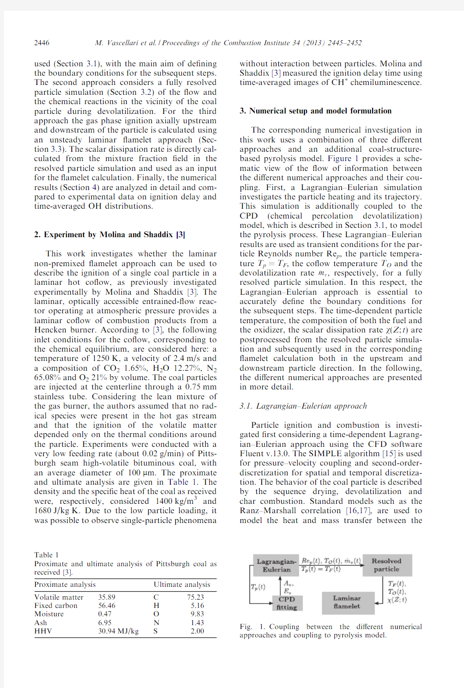
The corresponding numerical investigation in this work uses a combination of three di?erent approaches and an additional coal-structure-based pyrolysis model.Figure1provides a sche-matic view of the?ow of information between the di?erent numerical approaches and their cou-pling.First,a Lagrangian–Eulerian simulation investigates the particle heating and its trajectory. This simulation is additionally coupled to the CPD(chemical percolation devolatilization) model,which is described in Section3.1,to model the pyrolysis process.These Lagrangian–Eulerian results are used as transient conditions for the par-ticle Reynolds number Re p,the particle tempera-ture T p=T F,the co?ow temperature T O and the devolatilization rate_m v,respectively,for a fully resolved particle simulation.In this respect,the Lagrangian–Eulerian approach is essential to accurately de?ne the boundary conditions for the subsequent steps.The time-dependent particle temperature,the composition of both the fuel and the oxidizer,the scalar dissipation rate v(Z;t)are postprocessed from the resolved particle simula-tion and subsequently used in the corresponding ?amelet calculation both in the upstream and downstream particle direction.In the following, the di?erent numerical approaches are presented in more detail.

https://www.360docs.net/doc/9818661981.html,grangian–Eulerian approach

Particle ignition and combustion is investi-gated?rst considering a time-dependent Lagrang-ian–Eulerian approach using the CFD software Fluent v.13.0.The SIMPLE algorithm[15]is used for pressure–velocity coupling and second-order-discretization for spatial and temporal discretiza-tion.The behavior of the coal particle is described by the sequence drying,devolatilization and char combustion.Standard models such as the Ranz–Marshall correlation[16,17],are used to model the heat and mass transfer between the

Table1

Proximate and ultimate analysis of Pittsburgh coal as received[3].

Proximate analysis Ultimate analysis Volatile matter35.89C75.23 Fixed carbon56.46H 5.16 Moisture0.47O9.83 Ash 6.95N 1.43 HHV30.94MJ/kg S

2.00

2446M.Vascellari et al./Proceedings of the Combustion Institute34(2013)2445–2452

non-resolved particle and the surrounding gas phase.It is important to note that these correla-tions for momentum,heat and mass exchange were developed for non-reacting particles and it can be expected that reactions can modify the boundary layer around the particle.

The devolatilization rate is modeled based on an empirical single kinetic rate law[18]

dY

dt

?A v expeàE v=RT pTáeY0àYTe1T

where T p is the particle temperature and Y and Y0 are the instantaneous and the overall volatile yield on a dry ash-free(daf)basis,respectively.The model parameters A v and E v are the pre-exponen-tial factor and the activation energy,which need to be adjusted for the given coal and the operating conditions.Here,the CPD model[19]is used to determine the rate constants for the Pittsburgh coal.The CPD model requires chemical structure data from13C nuclear magnetic resonance(13C NMR)spectroscopy on the speci?c coal.Since these detailed analysis data are usually not avail-able,Genetti et al.[20]developed a non-linear correlation based on existing13C NMR data for 30coals to determine the required(coal-struc-ture-dependent)input data for the CPD model using the available proximate and ultimate analy-sis.This correlation is applied here.Initially,the coal particle temperature during devolatilization is estimated by means of an initial Lagrangian–Eulerian simulation(see Fig.1).In the next step, the single-rate pre-exponential factor A v and the activation energy E v are determined based on the CPD results(calculated with a separate code) using the particle heating rate from the Lagrang-ian–Eulerian simulation.This procedure is re-peated until convergence is reached,as shown by the feedback loop in Fig.1.Finally,the CPD re-sults are used to determine the total volatile yield at a high temperature,here54.75%daf:this is substantially higher than the38.86%from the proximate analysis obtained under the signi?-cantly di?erent standard heating conditions,as re-ported in Table1.The CPD?tting yields the?nal pre-exponential factor A v=72054.9sà1and the activation energy E v=54.285kJ/mol.The CPD gives results consistent with the FG-DVC model as reported in[21]in terms of devolatilization rate and volatile yield for the Pittsburgh coal.In gen-eral,the composition shown by both the FG-DVC and the CPD approach include higher hydrocarbons.However,in terms of modeling, this would require large chemical mechanisms, especially for the resolved particle simulation. Since the focus here is on the applicability of the ?amelet model and only partially on fully match-ing the experimental result,a composition with up to C2-hydrocarbons is chosen.

The volatile matter is assumed to be composed of CO,CH4,N2and C2H2,as reported in Table2.A kinetic mechanism including C2-hydrocarbons is necessary to satisfy the mass balance of ele-ments from the ultimate analysis.Oxygen in the volatile matter is completely assigned to CO,while the remaining carbon and hydrogen is split up between CH4and C2H2.The heat of pyrolysis resulting from this volatile composition in order to ful?ll the energy balance based on the given coal heating value is2.47MJ/kg,which represents the energy required during depolymerization.It is important to note that the assumed composition is arbitrary to a certain degree and is not prescribed by the CPD model directly.However,the same composition is also used for the resolved particle calculation and the?amelet calculation to ensure maximum consistency.Other approaches[22,23] which are also based on network models of coal devolatilization,could yield slightly di?erent com-positions and heats of pyrolysis.

The DRM mechanism[24]with103reactions among22chemical species is chosen here.This mechanism is used both for the resolved particle approach and the?amelet approach.Other mech-anisms such as GRI-MECH3.0are too computa-tionally expensive for the resolved particle approach.Therefore,the DRM mechanism is considered as a compromise between accuracy and computational cost.

It is important to note that the choice of CPD model and the chemical mechanism does not only in?uence the Lagrangian–Eulerian calculation, but the results are used directly and indirectly in the resolved particle simulation and the?amelet simulation.

3.2.Resolved particle approach

In a second step,ignition is modeled consider-ing a detailed laminar simulation fully resolving the?ow/mixing?eld and the chemical reactions around the coal particle using ANSYS Fluent v.13.0.The SIMPLE algorithm[15]is used for pressure–velocity coupling and second order dis-cretization for spatial and temporal discretization. The chemistry solver is used in combination with the ISAT algorithm[25].

A two-dimensional axisymmetric domain is considered(Fig.2),which extends from100 particle diameters upstream to200diameters Table2

Volatile matter composition

assumed for numerical simula-

tion(%weight).

Volatile matter composition

C2H20.420

CH40.282

CO20.269

N20.028

M.Vascellari et al./Proceedings of the Combustion Institute34(2013)2445–24522447

downstream and75diameters in a cross-stream direction.The computational grid consists of 190,000hexahedral cells and was re?ned several times in the ignition zone until a grid-independent unsteady solution was obtained.A time step is considered of1?10à5s with50iterations for each time step is considered.The oxidizer enters the domain on the left side with a constant com-position as previously described.The inlet velocity and the temperature vary during the simulation in accordance with the results of the Lagrangian–Eulerian simulation.Volatile matter is released from the particle surface with a time-dependent mass?ow rate and temperature postprocessed from the Lagrangian–Eulerian results.

For the subsequent?amelet analysis,an addi-tional balance equation is solved for the mixture fraction as a passive scalar

q @Z

@t

tq v a

@Z

@x a

?

@

@x a

q D Z

@Z

@x a

;e2T

where the di?usion coe?cient D Z is chosen as equal to the thermal di?usivity(Le Z=1)and the boundary conditions are Z=1at the particle surface and Z=0in the co?ow inlet.In addition, the scalar dissipation rate v=2D Z(o Z/o x a)2 required for the?amelet analysis,see Fig.1,is directly computed from the resolved mixture fraction?eld.

https://www.360docs.net/doc/9818661981.html,minar?amelet approach

An unsteady laminar?amelet approach is used to analyze the results of the resolved particle sim-ulation.This general approach considering a highly resolved simulation,e.g.a DNS,to evalu-ate and validate models for?amelet,CMC or other phenomena has been used previously in sev-eral areas,see e.g.[26–28]for gaseous turbulent auto-ignition.

A?amelet calculation of the gas phase ignition process is performed both in the upstream and the downstream particle direction using the corre-sponding scalar dissipation rate from the resolved particle simulation.This procedure allows the ?amelet approach to be evaluated as a potential submodel for application in turbulent coal?ames.

A recent overview of?amelet modeling is given in[29]and only a brief description is presented https://www.360docs.net/doc/9818661981.html,ing either a local coordinate transforma-tion or a two-scale asymptotic analysis,the?am-elet equations for the species mass fractions and the temperature with the mixture fraction Z as the independent variable are derived from the 3D balance equations,see Eq.(3)for the species mass fraction

q

@Y i

@t

àq

v

2Le i

@2Y i

@Z2

?_m i:e3T

Transport e?ects are described using the scalar dissipation rate v(Z).Here,we directly use the solution of the mixing?eld,see Eq.(2),to com-pute the scalar dissipation rate instead of using an analytical solution of a laminar counter-?ow ?ame(e.g.an inverse complementary error func-tion);this will be discussed below.In the follow-ing,both for the?amelet calculation and the resolved particle calculation,Le i=1was used for all species.Calculations using multicomponent di?usion coe?cients and corresponding averaged Le numbers showed a negligible e?ect on the igni-tion time.

4.Results and discussion

Figure3shows the particle temperature and the non-dimensional mass depletion as a function of time from the Lagrangian–Eulerian simulation indicating the drying(I),devolatilization(II)and char burnout(III)phases.The time t=0is de?ned as the moment the coal particle is injected into the reactor.The experimentally observed time period of CH*chemiluminescence[3]is high-lighted in gray.At0.034s,which is substantially later than the experimentally observed ignition delay of0.028s,the particle temperature increases rapidly after gas phase ignition.Since the Lagrangian–Eulerian approach cannot resolve the boundary layer,where the ignition takes

place

2448M.Vascellari et al./Proceedings of the Combustion Institute34(2013)2445–2452

in the case of a single particle,the ignition delay time is not expected to be close to the experimen-tal value.As mentioned above,the results from the Lagrangian–Eulerian simulation mainly pro-vide the boundary conditions for the resolved sim-ulation of the coal particle boundary layer?ow.

As shown in Fig.1,the time-dependent relative gas-particle velocity and the gas temperature from the Lagrangian–Eulerian simulation are used as boundary conditions for the upstream velocity inlet in the resolved particle simulation,which is schematically illustrated in Fig.2.In addition, the time-dependent particle temperature and dev-olatilization mass?ow rate are used as boundary conditions for the particle surface.Since ignition in the gas phase takes place during devolatiliza-tion,only this phase is considered here.In partic-ular,the calculation starts at0.015s,when1%of volatile matter was released,and ends at0.043s, when char combustion begins.

It is important to note that since the Lagrang-ian–Eulerian simulation overpredicts the ignition delay,the particle temperature provided to the resolved particle simulation is underpredicted dur-ing the later stages.However,a preliminary anal-ysis performed using the resolved particle approach and the?amelet approach showed that the particle temperature had a small e?ect on the ignition.This can be explained by the fact that ignition takes place at very lean mixtures Z ign

Figure4shows the results of the resolved coal particle simulation considering six time steps from 0.0235to0.0240s.Contours of temperature,OH mass fraction and the isoline of the stoichiometric mixture fraction are plotted.As will be discussed below in detail,ignition starts on the lean side and,as expected,in the downstream region.This is followed by a propagation both towards the stoichiometric mixture and around the particle. Considering the same time steps,Fig.5compares the temperature in the mixture fraction space both for the resolved particle simulation and the lami-nar?amelet simulation in the downstream direc-tion.An initial small increase in the temperature can be observed at0.0235s at Z=0.02,which corresponds to24diameters downstream.This is followed by a propagation towards the stoichiom-etric mixture Z st=0.1295,where the?ame becomes established as a regular di?usion?ame. In general,very good agreement can be observed between the results of the two simulation approaches in terms of ignition time and temper-ature pro?les.Only minor di?erences can be observed https://www.360docs.net/doc/9818661981.html,ing these data,it is interesting to note that the di?u-sion?ame structure,in particular,cannot be resolved with the Lagrangian–Eulerian approach. The?nal?ame stand-o?distance is0.7mm,which is close to the CFD cell size(a smaller CFD cell size is not feasible due to the particle diameter of0.1mm).Thus,the gradients in the?ame region cannot be resolved.This can only be achieved in the resolved particle simulation and the?amelet simulation.Figure5also shows the time-dependent scalar dissipation rate pro?les taken from the resolved particle simulation,which are used as input for the?amelet analysis.The maximum values are found at Z=1,which results from large mixture fraction gradients near the particle surface.These pro?les di?er signi?cantly from standard pro?les,which are usually zero at either boundary.Here,similar to droplet evapora-tion,transport processes take place at the bound-ary which must be described using the scalar dissipation rate in a?amelet simulation.The scalar dissipation decreases quickly towards the oxidizer side.

Ignition takes place on the lean side,which can be explained considering the higher temperature of the oxidizer compared to the fuel temperature, see e.g.[26].Furthermore,this ignition process is strongly dominated by the high scalar dissipation rate,as reported in Fig.5,which drops rapidly towards Z=0.In fact,a high scalar dissipation rate can even prevent auto-ignition,see e.g.the established S-curve for di?usion?ames.

It is interesting to note that a?amelet calcula-tion using a zero scalar dissipation rate yields an ignition time of0.022s and therefore signi?cantly underpredicts the ignition delay.On the other hand,using the inverse complementary error function(erfcà1)pro?le[29](which is the analyti-cal solution for a counter?ow?ame)scaled with the transient stoichiometric value v st(t)taken from the resolved particle simulation strongly overpre-dicts the ignition onset.This is due to the higher v-values on the lean side compared to the pro?le taken from the resolved particle simulation.Thus, using the stoichiometric scalar dissipation rate only is not feasible here since ignition takes place far away from stoichiometry in the?amelet space. Consequently,for the investigated conditions the laminar?amelet approach can accurately predict ignition only if considering accurate scalar dissi-pation pro?les are considered.

In Fig.6,the mass fractions of several species for the same time steps as shown in Figs.4and 5are compared for the resolved particle simula-tion and the?amelet simulation.Again,the results show good agreement and only minor dif-ferences can be observed from0.0236to0.0239s, which is comparable to the results presented in Fig.5.

As expected,using the same?amelet procedure for the upstream direction fails to capture the igni-tion process(not shown here)and yields a signif-icantly higher delay.This is due to the higher scalar dissipation rates upstream,which prevent auto-ignition completely,both in the resolved par-ticle simulation and in the?amelet calculation. The upstream ignition is caused by the?ame

M.Vascellari et al./Proceedings of the Combustion Institute34(2013)2445–24522449

propagation around the particle,which can be seen in Fig.4.This propagation cannot be described with a 1D unsteady ?amelet approach,which can only describe auto-ignition processes in its present formulation.However,once ignition takes place,resolved particle simulation and ?am-elet simulations show good agreement in terms of temperature and chemical species for the burning di?usion ?ame.This overall agreement for the resolved particle simulation and the ?amelet approach is an encouraging result for the future use of the ?amelet approach as a submodel for turbulent coal combustion simulations.

Figure 7compares the ignition delay calculated from the resolved particle simulation with the experimental result.[3]measured ignition by means of CH *chemiluminescence data,correlat-ing the position of the radical peak with time based on the particle https://www.360docs.net/doc/9818661981.html,ing the trajec-tory,the particle position can be directly con-verted to the residence time.Since the DRM mechanism does not include CH,the OH radical was considered instead in the numerical simula-tion to predict the ignition onset in a similar way to that in the experiments.Additional lami-nar ?amelet simulations (not shown here)with more detailed mechanisms such as GRI-MECH 3.0,which included CH as representative for CH *,showed that OH and CH onsets happen almost simultaneously,but for slightly di?erent mixture fraction values.The qualitative compari-son also shows that the numerical results predict earlier ignition at approximately 0.024s compared to the experiments,which elicit 0.028s.

However,

Contour plots of temperature,OH mass fraction and the stoichiometric mixture fraction isoline obtained resolved particle simulation for six time steps from 0.0235to 0.024s.

the overall agreement between the numerical and experimental results can be considered quite good,considering the complexity of both coal combus-tion experiments and simulations.5.Summary and conclusions

The ignition of a single coal particle in a lami-nar hot co?ow was investigated using a combina-tion of three di?erent numerical approaches,and the results were compared to available experimen-tal data.First,the transient behavior of the coal particle was simulated with a Lagrangian–Euleri-an approach,which was coupled with a detailed pyrolysis model.The results were postprocessed to provide appropriate transient boundary condi-tions as an input for a simulation fully resolving the ?ow/mixing ?eld and the chemical reactions in the vicinity of the particle.The results of the resolved particle simulation showed good agree-ment with the experimental data for the ignition delay time,especially considering the inherent uncertainties of coal combustion experiments.Finally,ignition was investigated downstream of the particle considering an unsteady non-premixed laminar ?amelet approach with time-

dependent scalar dissipation pro?les evaluated from the resolved particle calculation.Very good results were obtained in terms of ignition delay,temperature and species pro?les during ignition and for the resulting di?usion ?ame comparing the latter two numerical approaches.As can be expected,the 1D ?amelet could not capture the subsequent ignition in the upstream region,which is caused by a ?ame propagation around the par-ticle.The results con?rm the general applicability of the laminar ?amelet approach to correctly pre-dict coal particle ignition during devolatilization,which is an encouraging result for using ?amelets as a submodel for turbulent coal combustion sim-ulations.In addition,the current results show clearly the importance of using the correct scalar dissipation rate pro?https://www.360docs.net/doc/9818661981.html,ing standard pro?les such as inverse complementary error function,originally derived for a counter?ow con?guration,yields signi?cantly di?erent and less accurate results.

Acknowledgments

The authors gratefully acknowledge the ?nan-cial support from the Federal Ministry of Educa-tion and Research in the framework of Virtuhcon (Project No.03Z2FN11).

The authors also thank Chris Shaddix for pro-viding the experimental data and Oliver Stein for helpful discussions.References

[1]R.H.Essenhigh,M.K.Misra,D.W.Shaw,Com-bust.Flame 77(1989)3–30.

[2]W.McLean,D.Hardesty,J.Pohl,https://www.360docs.net/doc/9818661981.html,bust.Inst.18(1981)1239–1248.

[3]A.Molina,C.R.Shaddix,https://www.360docs.net/doc/9818661981.html,bust.Inst.31(2007)1905–1912.

[4]C.R.Shaddix,A.Molina,https://www.360docs.net/doc/9818661981.html,bust.Inst.32(2009)

2091–2098.

M.Vascellari et al./Proceedings of the Combustion Institute 34(2013)2445–24522451

[5]P.A.Bejarano,Y.A.Levendis,Combust.Flame153

(2008)270–287.

[6]R.Khatami,C.Stivers,K.Joshi,Y.A.Levendis,

A.F.Saro?m,Combust.Flame159(2012)1253–

1271.

[7]Y.A.Levendis,K.Joshi,R.Khatami,A.F.Saro?m,

Combust.Flame158(2011)452–465.

[8]L.Zhang,E.Binner,Y.Qiao,C.-Z.Li,Energy

Fuels24(2009)29–37.

[9]L.Zhang,E.Binner,L.Chen,et al.,Energy Fuels

24(2010)4803–4811.

[10]T.Joutsenoja,J.Saastamoinen,M.Aho,R.Hern-

berg,Energy Fuels13(1999)130–145.

[11]X.Du,K.Annamalai,Combust.Flame97(1994)

339–354.

[12]M.Zhu,H.Zhang,Z.Zhang,D.Zhang,Combust.

Sci.Technol.183(2011)1221–1235.

[13]C.Wendt, C.Eigenbrod,O.Moriue,H.Rath,

https://www.360docs.net/doc/9818661981.html,bust.Inst.29(2002)449–457.

[14]F.Higuera,Combust.Flame156(2008)1023–1034.

[15]S.Patankar,Numer.Heat Transfer A4(1981)

409–425.

[16]M.Ranz,W.R.Marshall,Chem.Eng.Prog.48

(1952)141–146.

[17]M.Ranz,W.R.Marshall,Chem.Eng.Prog.48

(1952)173–180.[18]S.Badzioch,P.Hawksley,Ind.Eng.Chem.Process

Des.Dev.9(1970)521–530.

[19]D.Grant,R.Pugmire,T.Fletcher,A.Kerstein,

Energy Fuels3(1989)175–186.

[20]D.Genetti,T.Fletcher,R.Pugmire,Energy Fuels

13(1999)60–68.

[21]R.Backreedy,R.Habib,J.Jones,M.Pourkasha-

nian,Fuel78(1999)1745–1754.

[22]S.Niksa,A.Kerstein,Energy Fuels5(1991)647–

665.

[23]P.R.Solomon,M.A.Serio,E.M.Suuberg,Prog.

Energy Combust.18(1992)133–220.

[24]A.Kazakov,M.Frenklach,Reduced Reaction Sets

based on gri-mech1.2,1994,available at http:// https://www.360docs.net/doc/9818661981.html,/drm/.

[25]S.Pope,Combust.Theory Model.1(1997)41–63.

[26]E.Mastorakos,T.Baritaud,T.Poinsot,Combust.

Flame109(1997)198–223.

[27]R.Hilbert, D.The′venin,Combust.Flame128

(2002)22–37.

[28]V.Mittal,D.J.Cook,H.Pitsch,Combust.Flame

(2012).

[29]N.Peters,Turbulent Combustion,Cambridge Uni-

versity Press,2000.

2452M.Vascellari et al./Proceedings of the Combustion Institute34(2013)2445–2452