Analysis of networked control systems with drops and variable delays

Automatica43(2007)2054–

2059

https://www.360docs.net/doc/b18455918.html,/locate/automatica

Brief paper

Analysis of networked control systems with drops and variable delays?

Matías García-Rivera?,Antonio Barreiro

Departamento de Ingeniería de Sistemas y Automática,E.T.S.Ingenieros Industriales,Universidad de Vigo,36200Vigo,Spain

Received3April2006;received in revised form4December2006;accepted30March2007

Available online10September2007

Abstract

Motivated by the insertion of a communication network in the feedback control loop,this paper focuses on how network-induced data dropouts and variable delays affect the stability of a linear plant with state feedback control.Suf?cient conditions for Lyapunov stability are derived in the case of uncertainty due to drops and delays.The veri?cation problem of the suf?cient conditions can be directly cast as an LMI feasibility problem.We illustrate the methodology by an example in the cases of drops,delays and drops with delays.

Keywords:Networked control systems(NCS);Data dropout;Delays;Robustness;Lyapunov stability;Linear matrix inequality(LMI)

1.Introduction

The fundamental purpose of data networks is to provide ac-cess to shared resources,most notably computers(Tanenbaum, 1996),but sensors,actuators and controllers can be equipped with network interfaces,and thus became independent nodes on a real-time control network.A networked control system(NCS) is a closed-loop control system over a data network(Tipsuwan &Chow,2003;Zhang,Branicky,&Phillips,2001;Walsh&Ye, 2001).All the information(reference input,plant output,con-trol input,etc.)is exchanged using a https://www.360docs.net/doc/b18455918.html,works reduce the complexity in wiring connections and the costs of medias, and provide ease in maintenance.Many different network types have been promoted for use in control systems(Lian,Moyne, &Tilbury,2001):general networks such as Ethernet and wire-less extensions,and specialized networks such us CAN and ControlNet.

A communication network in the feedback-control loop makes the analysis of NCS complex.Conventional control

?This paper was not presented at any IFAC meeting.This paper was recommended for publication in revised form by Associate Editor Denis Dochain under the direction of Editor Frank Allg?wer.Work supported by CICYT,Spain,DPI04-07670-CO2-01.

?Corresponding author.

E-mail addresses:mgrivera@uvigo.es(M.García-Rivera),

abarreiro@uvigo.es(A.Barreiro).

0005-1098/$-see front matter?2007Elsevier Ltd.All rights reserved. doi:10.1016/j.automatica.2007.03.027theories suppose ideal assumptions,such as no drops and no delays from sensors to actuators.The network-induced drops and delays can degrade the performance of control systems designed without considering them,and can even destabilize the system.

Halevi and Ray(1988)consider a continuous-time plant with discrete-time controller and analyze the system using a discrete-time approach.The system is represented by an augmented state vector that consists of past and current values of inputs and outputs of the plant and controller.Nilsson(1998)in a discrete-time domain modelled network delays as constant,in-dependently random,and random but governed by a underlying Markov chain.The LQG optimal control problem is solved for these delay models.Delays are not random,but depend on vari-ous aspects(Colandairaj,Scanlon,&Irwin,2005),for example network load,which increases when the sampling period de-creases.Walsh,Ye,and Bushnell(1999)consider a continuous plant and a continuous controller.They introduce the notion of maximum allowable transfer interval(MATI),denoted by , which supposes that successive sensor messages are separated by at most seconds.

Network data transmision paths are unreliable,packets can be lost during transmision and it can affect the performance of the NCS.In(Hassibi,Boyd,&How,1999;Zhang,2001; Zhang et al.,2001),dropouts are modelled as an asynchronous dynamical systems(ADS).They require a Lyapunov-type

M.García-Rivera,A.Barreiro/Automatica43(2007)2054–20592055

function to decrease on the average along state trajectories of the asynchronous system.Another contribution found in (Nilsson,1998)models dropouts as a Markov chain,and uses past control signals or estimated lost data to computing the new control signals.

To date,most authors have studied the in?uence of delays with a continuous or discrete time approach,and only a few works have been made about drops.

The main contribution of this paper is to study both drops and delays with a discrete time approach.We present a new way how the uncertainty due to drops and delays is embedded, leading to suf?cient stability conditions based on LMIs,solved using available tools(Boyd,El Ghaoui,Feron,&Balakrishnan, 1994;Gahinet,1995).

The layout of this paper is as follows.In Section2,issues about NCS and Lyapunov-based methods are addressed.Sec-tion3shows how uncertainty is treated in the case of drops,and a suf?cient stability condition is presented.Uncertainty and suf-?cient stability conditions are shown for variable delays,Sec-tion4,and variable delays with drops,Section5.Conclusions are drawn in Section6.

2.Preliminaries

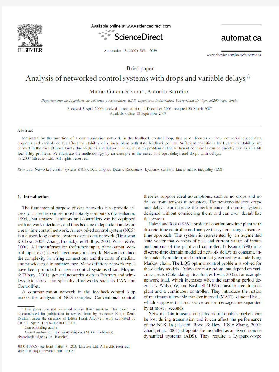
The NCS considering network-induced drops and delays is shown in Fig.1.The linear continuous plant is

˙x(t)=A x(t)+B u(t),y(t)=C x(t)(1) and the controller u(t)=?K x(t),where x(t)∈R n is the state of the plant,u(t)∈R p the controlled input and y(t)∈R q the output;A,B,C and K are matrices of appropiate sizes.We as-sume that the control system has been designed without having the network in mind.That is,the original continuous plant and the continuous state feedback controller without the network connection is stable or satis?es certain control speci?cations. There are two sources of delays in the network:sensor to controller, sc,and controller to actuator, ca.Any controller delay can be absorbed into either sc or ca,without loss of generality.For time-invariant controllers,both delays can be lumped together as = sc+ ca.

We consider the following setup:a clock-driven sensor,that periodically samples the plant outputs;an event-driven con-troller,which calculates the control signal as soon as the sen-sor data arrive;an event-driven actuator,that changes the

plant

https://www.360docs.net/doc/b18455918.html,worked control system.inputs as soon as the controller data arrive;the total delay between sensor and actuator is smaller than the sampling period, h.

Sampling the plant given by(1)with period h(˙Astr?m& Wittenmark,1997),we obtain x k+1= x k+ u k.The resulting discrete time linear time invariant control system is x k+1=A x k, where

A=( ? K),(2)

= (h)=e Ah, = (h)=

e As d sB.(3)

In the following sections,we will change Eqs.(2)and(3)to incorporate drops and delays.We assume that the maximum number of consecutive drops and the maximum variable delay are known.

The stability criterion derived in this paper,is based on the well-known Lyapunov second method for determining the sta-bility of a system.Different classes of Lyapunov functions have been proposed in the control literature for analyzing dynamical systems.In this work we search over simple discrete quadratic Lyapunov functions,V(x k),given by V(x k)=x T k P x k,P>0. The control system with drops and delays will be modelled as a linear time varying system,given by x k+1=A k x k where A k∈{A1,A2,...,A N}.This varying system is said to be quadratically stable,if there exists a?xed quadratic Lyapunov function which veri?es P=P T>0and A T k P A k?P<0,?A k. The analysis techniques developed in this work have been applied to the following control system(Zhang et al.,2001)

˙x=

0?0.1

0.1

u,y=[10]x,

u=?[3.7511.5]x.(4) 3.Dropping samples

In a simple case,control inputs do not suffer delays but can be lost during transmission.Normally,feedback-controlled plants can tolerate a certain amount of data loss,therefore it is valuable to determine whether the system is stable as a function of D M,the maximum number of consecutive data drops that networks can induce.

Let us consider the time axis as a succession of intervals delimited by two consecutive control inputs that do arrive to the actuator of the plant.Let us de?ne I k(d k)=[kh,(k+d k+1)h] as an interval of order d k,where K is the sampling instant for which its corresponding control input u k arrives to the actuator, and d k is the number of consecutive control input drops between u k and the next control input that arrives to the plant,u k+d

k+1

. Therefore,there are d k control input drops between u k and u k+d

k+1

.Fig.2shows some intervals with no drops,I k?1(0), I k+2(0)and I k+6(0),one interval with one drop,I k(1),and one interval with two drops,I k+3(2).In this case,the control inputs u k+1and the two consecutive u k+4and u k+5,never arrive to the plant.

The control system will be analyzed as the following linear time variant system,taking the sampling period multiples of

2056M.García-Rivera,A.Barreiro /Automatica 43(2007)2054–

2059

Fig.2.Dropping of one and two consecutive control inputs.

0.20.40.60.81

1.2 1.4 1.6 1.8

024********

16h [s]

Fig.3.Quadratic stability region for drops.

the basic period h ,that is,{h,2h,...}x k +d k +1= d k x k + d k u k ,

(5)

where d k and d k come from (3), d k = ((d k +1)h)and d k = ((d k +1)h).If a state-feedback control is applied,u k =?K x k ,expression (5)can be rewritten as x k +d k +1=A d k x k ,where

A d k = d k ? d k K = ((d k +1)h)? ((d k +1)h)K .In the case of control input drops,the system will be stable up to m consecutive data drops,if there exists a P =P T >0such that,A T d k P A d k

?P <0,

0 d k m .

A simple method for testing if D M consecutive data drops in a network give a stable system,is to check the feasibility of the following set of LMIs P =P T >0,A T d k P A d k ?P <0,

0 d k D M .

(6)

The quadratic stability region is the set of values for which the control system veri?es equation (6),and therefore,it is stable.In the case of dropping samples,the quadratic stability region for the system given by (4)is represented in Fig.3.A point is marked in the location of the combinations of h and D M for which (6)holds.D M =0represents the no dropping case,and therefore,the maximum stable sampling period is 1.729s (Zhang et al.,2001).It should be pointed out that Fig.3is

only for analysis purpose.The parameter h is not free for the designer,it is imposed by the dynamics of the plant and the performance required in the control system.4.Variable delays

Transmision delay in a data network varying from transfer to transfer,represents a more realistic case.Again,feedback-controlled plants can tolerate a certain amount of variable delay,therefore is valuable to determine whether the system is stable as a function of the maximum variable delay, M .Even for non-deterministic networks,end-to-end delays can be upper-bounded (Georges,Divoux,&Rondeau,2005).

Let us consider that the variable delay of each sample, k ,satis?es 0 k M h,?k .Sampling the continuous system

with period h ,we obtain (˙Astr?m &Wittenmark,1997)x k +1= x k + 0( k )u k + 1( k )u k ?1,where is de?ned in (3)and

0( k )= h ? k

e As d sB .

(7) 1( k )=e A(h ? k )

e As d sB .

(8)

De?ning z k =[x T k u T k ?1]T ,as the augmented state vector,the

augmented open-loop system is

z k +1= 1( k )00 z k + 0( k )

u k .

(9)If u k =?K x k is the feedback gain for the system with no

delay,then the augmented gain for the augmented state vector will be u k =?[K 0]z k .The augmented closed-loop system is z k +1=A( k )z k (Zhang et al.,2001),where

A( k )= ? 0( k )K 1( k )

?K 0 .(10)

This linear time variant system will be stable if there exists a

P =P T >0that veri?es A T ( k )P A( k )?P <0,

0 k M

(11)

therefore,a system with an in?nite number of LMIs should be solved.This is a untractable problem (Blondel &Tsitsiklis,2000)and we will search a suf?cient condition for the stability of the system with a variable delay k between 0and M ,solving a ?nite number of LMIs.

The matrix of the autonomous system (10)can be given as a function of 0( k ),removing 1( k )using (A.1),

A( k )=

? 0( k )K ? 0( k )

?K 0

and the Lyapunov matrix can be rewritten as P =[P 1P 2;P T 2

P 3],where P is (n +p)×(n +p),P 1is n ×n ,n is the dimension

M.García-Rivera,A.Barreiro /Automatica 43(2007)2054–20592057

of x k and p is the dimension of u k ?1.Therefore,expression (11)is written as

A T

( k ) P 1P 2P T 2P 3 A( k )? P 1P 2P T 2P 3

<0,which amounts to the fact that for all x k and u k ?1

x k u k ?1 T

A T ( k )

P 1

P 2

P T 2

P 3

A( k )?

P 1P 2

P T 2

P 3

× x k u k ?1

from which we get

x T k (( ? 0( k )K)T

P 1( ? 0( k )K)

?2K T P T

2( ? 0( k )K)+K T P 3K ?P 1)x k

+2u T k ?1(( ? 0( k ))T

P 1( ? 0( k )K)

?( ? 0( k ))T P 2K ?P T

2)x k

+u T k ?1(( ? 0( k ))T

P 1( ? 0( k ))?P 3)u k ?1<0

and,reordering terms

x T k ( T P 1 ?2 T P 1 0( k )K +K T T 0( k )P 1 0( k )K

?2K T P T 2 +2K T P T

2 0( k )K +K T P 3K ?P 1)x k

+2u T k ?1( T P 1 ? T P 1 0( k )K ? T

0( k )P 1

+ T 0( k )P 1 0( k )K ? T P 2K + T 0( k )P 2K ?P T 2)x k

+u T k ?1( T P 1 ? T 0( k )P 1 ? T

0( k )P 1

+ T 0( k )P 1 0( k )?P 3)u k ?1<0.

(12)

Reordering (12),we get Q( 0( k ))+L( 0( k ))+C <0,where Q is real-valued quadratic function of 0( k ),L is real-valued linear function of 0( k ),and C is real number independent of 0( k ).These terms are given by C

=x T k ( T P 1 ?2K T P T 2 +K T

P 3K ?P 1)x k

+2u T k ?1( T P 1 ? T P 2K ?P T

2)x k

+u T k ?1( T

P 1 ?P 3)u k ?1,

L( 0( k ))=x T k (?2 T P 1 0( k )K +2K T P T 2 0( k )K)x k

+2u T k ?1(? T P 1 0( k )K ? T

0( k )P 1 + T 0( k )P 2K)x k u T k ?1(? T 0( k )P 1

? T 0( k )P 1 )u k ?1,

Q( 0( k ))=x T k K T T

0( k )P 1 0( k )K x k

×2u T k ?1 T 0( k )P 1 0( k )K x k +u T k ?1 T 0( k )P 1 0( k )u k ?1

=(K x k +u k ?1)T T 0( k )P 1 0( k )(K x k +u k ?1).

(13)

If p =dim (u k ?1)=1,from Eq.(13)we get Q( 0( k ))=a 0( k )T P 1 0( k )where a =||(K x k +u k ?1)||2>0.Also,L( 0( k ))=B T (x k ,u k ?1) 0( k )= b i (x k ,u k ?1) i 0( k )

()

Fig.4. 0,1, 0,2and 0,3for h =0.5s,0 k 0.25.

where B =[b 1,...,b n ]T and i 0( k )are the coef?cients of

0( k ).Expression (12)can be rewritten as a T 0( k )P 1 0( k )+B T 0( k )+C <0where P 1and aP 1are positive de?nite.Therefore,the set of solutions for this quadratic form is a con-vex region.

0( k )can not take any value because it is a curve in R n for k .A set of vertices,{ 0,1,..., 0,J }∈R n ,can be found such 0( k )belongs to the convex hull co { 0,1,..., 0,J },0 k M .LMIs can analyze the stabil-ity with variable delays.The system is stable for a sampling period h ,and a variable delay ∈[0, M ]if there exists a P solution for the following set of LMIs P =P T >0

A T ( 0,j )P A( 0,j )?P <0?j =1,...,J ,(14)

where

A( 0,k )=

? 0,k K

? 0,k

.If the LMI (14)is feasible,its solution P is valid for (11)

from the fact 0( k )∈co { 0,1,..., 0,J },0 k M .The keypoint is the demostrated convexity of (12)with respect to 0( k ).

Fig.4shows for the example in (4)and h =0.5s,the two

components of the curve 0( k )=[ 10( k ) 20( k )]T ,when k

varies from 0to h .It must be noted that for 0 k M ,the curve is closed inside the convex region given by the following three points

0,1= 10(0) 20(0) , 0,2= 10( M )

20( M ) ,

0,3= 10(0)

20( M ) .

Then,the system given by (4)is stable for a sampling period h ,and a variable delay k ∈[0, M ]if there exists a matrix P

2058M.García-Rivera,A.Barreiro /Automatica 43(2007)2054–2059

0.20.40.60.81

1.2 1.4 1.6 1.8

0102030405060708090

100h [s]

τ (%h )

Fig.5.Quadratic stability region for variable delay.

solution for the following set of LMIs P =P T >0,

A T ( 0,1)P A( 0,1)?P <0,A T ( 0,2)P A( 0,2)?P <0,A T ( 0,3)P A( 0,3)?P <0.

(15)

The quadratic stability region represents the combinations of h and M ,for which the system veri?es the expression (15).A point is marked in the location of the combination of h and M for which (15)is feasible.Fig.5shows the results of the system given by (4).

5.Variable delays with drops

In the most general case,control inputs arrive with a random delay and some of them are lost.With a maximum variable delay M ,0 k M h ?k ,and a maximum number of con-secutive drops D M ,0 d k D M ?k ,the behavior in I k (d k )is given by z k +d k +1=A d k ( k )z k where

A d k ( k )=

d k ? 0,d k ( k )K d k ? 0,d k ( k )

?K 0 (16)and 0,d k ( k )= (d k +1)h ? k 0e As

d sB .

Similarly as it was shown in Sections 3and 4,a system with variable delays and drops will be stable if there exits a P =P T >0such that,A T d k ( k )P A d k ( k )?P <0,

0 k M ,0 d k D M .(17)

Again,the variable delay results in an in?nite number of LMIs to be solved.As in Section 4a suf?cient condition can be found solving a ?nite number of LMIs.Therefore,the stability condition (17)can be rewritten as

P =P T >0,A T d k ( 0,j )P A d k ( 0,j )?P <0,1 j J,0 d k D M (18)

where

A d k ( 0,j )=

d k ? 0,d k ,j K

d k ? 0,d k ,j

and 0,d k ,j are a set of vertices that enclose 0,d k ( k )in a convex region.

0.5

1.5

6080

100

1015τv (%

h )h [s ]

Fig.6.Stability region for variable delays and drops.

The quadratic stability region represents now the combina-tions of h , M and D M ,for which the system satis?es the ex-pression (18).Results for (4)are shown in Fig.6.6.Conclusions

In this paper we have presented a discrete time approach to the robustness of a networked control system in the presence of random drops and delays.The uncertainty due to drops and delays is embedded within some limits,the maximum number of consecutive drops and the maximum variable delay.These limits leads to suf?cient stability conditions using common Lyapunov functions.The ful?llment of these suf?cient stabil-ity conditions can be cast and solved as an LMI feasibility problem.

The resulting suf?cient conditions can guarantee the stabil-ity for the cases of drops,variable delays and variable delays with drops.The obtained common Lyapunov functions always decrease along all the state trajectories of the system for any secuence of random drops and delays.Examples were also included to demostrate the effectiveness of this approach in analysing NCS.

This work is limited to a state feedback control with single input.The extension to an arbitrary number of inputs should consider the convex bounding of an n ×p 0( k ).A useful idea is some canonical form for A ,in this way the convex bound should be much easier to compute.However,the explicit and detailed construction of the convex bounds in all the general cases requires further research and will be considered in future work.

Appendix A.Proofs

The change of variable s =r ?(h ? )in (8)results

1( )=e A(h ? ) 0e As d sB =e A(h ? ) h

h ?

e A(r ?(h ? ))d rB

= h h ?

e Ar d rB = h h ?

e As d sB .

M.García-Rivera,A.Barreiro/Automatica43(2007)2054–20592059 Adding 0( )from(7)to 1( )

0( )+ 1( )= h?

e As d sB+

e As d sB

= 0(0)= .(A.1) References

˙Astr?m,K.J.,&Wittenmark,B.(1997).Computer-controlled systems:Theory and design.Englewood Cliffs,NJ:Prentice-Hall.

Blondel,V. D.,&Tsitsiklis,J.N.(2000).A survey of computational complexity results in systems and control.Automatica,36(9),1249–1274. Boyd,S.,El Ghaoui,L.,Feron,E.,&Balakrishnan,V.(1994).Linear matrix inequalities in system and control theory(V ol.15).In Studies in applied mathematics.SIAM.

Colandairaj,J.,Scanlon,W.G.,&Irwin,G.W.(2005).Co-simulation framework for a networked control system within an IEEE802.11b ad-hoc network.In Proceedings of16th IFAC world congress,Prague,Czech Republic.

Gahinet,P.,Nemirovshi,A.,Laub,A.,&Chilali,M.(1995).LMI toolbox: For use with MATLAB.MathWorks.

Georges,J.P.,Divoux,T.,&Rondeau, E.(2005).Confronting the performances of a switched ethernet network with industrial constraint by using the network calculus.International Journal of Communication Systems,877–903.

Halevi,Y.,&Ray,A.(1988).Integrated communication and control systems: Part I—analysis.ASME Journal of Dynamic Systems,Measurement and Control,110,367–373.

Hassibi,A.,Boyd,S.P.,&How,J.P.(1999).Control of asynchronous dynamical system with rate constraints on events.In Proceedings of the IEEE CDC(pp.1345–1351),Phoenix.

Lian,F.L.,Moyne,J.R.,&Tilbury,D.M.(2001).Performance evaluation of control networks:Ethernet,ControlNet and DeviceNet.IEEE Control Systems Magazine,21(1),66–84.

Nilsson,J.(1998).Real-time control systems with delays.Ph.D.dissertation, Lund Institute of Technology,1998.

Tanenbaum,A.S.(1996).Computer Networks.(3rd ed.),Upper Saddle River, NJ:Prentice-Hall.Tipsuwan,Y.,&Chow,M.-Y.(2003).Control methodologies in networked control systems.Control Engineering Practice,11(3),1099–1111. Walsh,G.C.,&Ye,H.(2001).Scheduling of networked control systems.

IEEE Control Systems Magazine,21(1),57–65.

Walsh,G.C.,Ye,H.,&Bushnell,L.(1999).Stability analysis of networked control systems.In Proceedings of American control conference(pp.

2876–2880),San Diego,CA.

Zhang,W.(2001).Stability analysis of networked control systems.Ph.D.

Thesis,Case Western Reserve University,2001.

Zhang,W.,Branicky,M.S.,&Phillips,S.M.(2001).Stability of networked control systems.IEEE Control Systems Magazine,21(1),

84–99.

Matías García Rivera was born in Vigo,

Spain,in1968.He received the M.S.degree in

Telecommunication Engineering and the Ph.D.

degree in System Engineering and Automation

from the University of Vigo,Spain,in1993and

2005,respectively.He joined the Department of

Systems Engineering and Automation in1995

where he is working as associate professor in

the?eld of computer science.His currently

research interests are in the areas of robust

stability,time-delay systems and networked

control.

Antonio Barreiro was born in Vigo,Spain,in

1959.He received the degrees of Ingeniero and

Doctor Ingeniero Industrial from the Polythec-

nic University of Madrid(UPM)in1984and

1989,respectively.From1984to1987he was

with the Departamento de Matemática Aplicada

of the E.T.S.Ingenieros Industriales of the UPM.

Since1987he has been with the Departamento

de Ingeniería de Sistemas y Automática of the

University of Vigo,where he is now Professor

in the?eld of Automatic Control.His research

interests include nonlinear and robust stability,

time-delay systems and networked control,with

applications on robotics,teleoperation and au-

tonomous vehicles.