twoScaleParticleSimulation
Two-Scale Particle Simulation
Barbara Solenthaler ETH Zurich Markus Gross ETH
Zurich
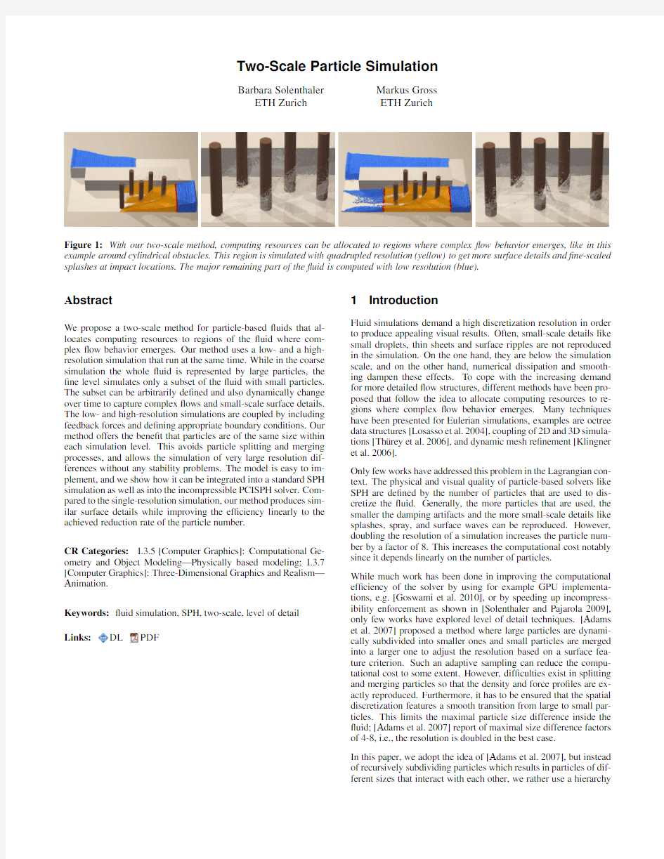
Figure1:With our two-scale method,computing resources can be allocated to regions where complex?ow behavior emerges,like in this example around cylindrical obstacles.This region is simulated with quadrupled resolution(yellow)to get more surface details and?ne-scaled splashes at impact locations.The major remaining part of the?uid is computed with low resolution(blue).
Abstract
We propose a two-scale method for particle-based?uids that al-
locates computing resources to regions of the?uid where com-
plex?ow behavior emerges.Our method uses a low-and a high-
resolution simulation that run at the same time.While in the coarse
simulation the whole?uid is represented by large particles,the
?ne level simulates only a subset of the?uid with small particles.
The subset can be arbitrarily de?ned and also dynamically change
over time to capture complex?ows and small-scale surface details.
The low-and high-resolution simulations are coupled by including
feedback forces and de?ning appropriate boundary conditions.Our
method offers the bene?t that particles are of the same size within
each simulation level.This avoids particle splitting and merging
processes,and allows the simulation of very large resolution dif-
ferences without any stability problems.The model is easy to im-
plement,and we show how it can be integrated into a standard SPH
simulation as well as into the incompressible PCISPH https://www.360docs.net/doc/cf7272778.html,-
pared to the single-resolution simulation,our method produces sim-
ilar surface details while improving the ef?ciency linearly to the
achieved reduction rate of the particle number.
CR Categories:I.3.5[Computer Graphics]:Computational Ge-
ometry and Object Modeling—Physically based modeling;I.3.7
[Computer Graphics]:Three-Dimensional Graphics and Realism—
Animation.
Keywords:?uid simulation,SPH,two-scale,level of detail
Links:
DL PDF
1Introduction
Fluid simulations demand a high discretization resolution in order
to produce appealing visual results.Often,small-scale details like
small droplets,thin sheets and surface ripples are not reproduced
in the simulation.On the one hand,they are below the simulation
scale,and on the other hand,numerical dissipation and smooth-
ing dampen these effects.To cope with the increasing demand
for more detailed?ow structures,different methods have been pro-
posed that follow the idea to allocate computing resources to re-
gions where complex?ow behavior emerges.Many techniques
have been presented for Eulerian simulations,examples are octree
data structures[Losasso et al.2004],coupling of2D and3D simula-
tions[Th¨u rey et al.2006],and dynamic mesh re?nement[Klingner
et al.2006].
Only few works have addressed this problem in the Lagrangian con-
text.The physical and visual quality of particle-based solvers like
SPH are de?ned by the number of particles that are used to dis-
cretize the?uid.Generally,the more particles that are used,the
smaller the damping artifacts and the more small-scale details like
splashes,spray,and surface waves can be reproduced.However,
doubling the resolution of a simulation increases the particle num-
ber by a factor of8.This increases the computational cost notably
since it depends linearly on the number of particles.
While much work has been done in improving the computational
ef?ciency of the solver by using for example GPU implementa-
tions,e.g.[Goswami et al.2010],or by speeding up incompress-
ibility enforcement as shown in[Solenthaler and Pajarola2009],
only few works have explored level of detail techniques.[Adams
et al.2007]proposed a method where large particles are dynami-
cally subdivided into smaller ones and small particles are merged
into a larger one to adjust the resolution based on a surface fea-
ture criterion.Such an adaptive sampling can reduce the compu-
tational cost to some extent.However,dif?culties exist in splitting
and merging particles so that the density and force pro?les are ex-
actly reproduced.Furthermore,it has to be ensured that the spatial
discretization features a smooth transition from large to small par-
ticles.This limits the maximal particle size difference inside the
?uid;[Adams et al.2007]report of maximal size difference factors
of4-8,i.e.,the resolution is doubled in the best case.
In this paper,we adopt the idea of[Adams et al.2007],but instead
of recursively subdividing particles which results in particles of dif-
ferent sizes that interact with each other,we rather use a hierarchy
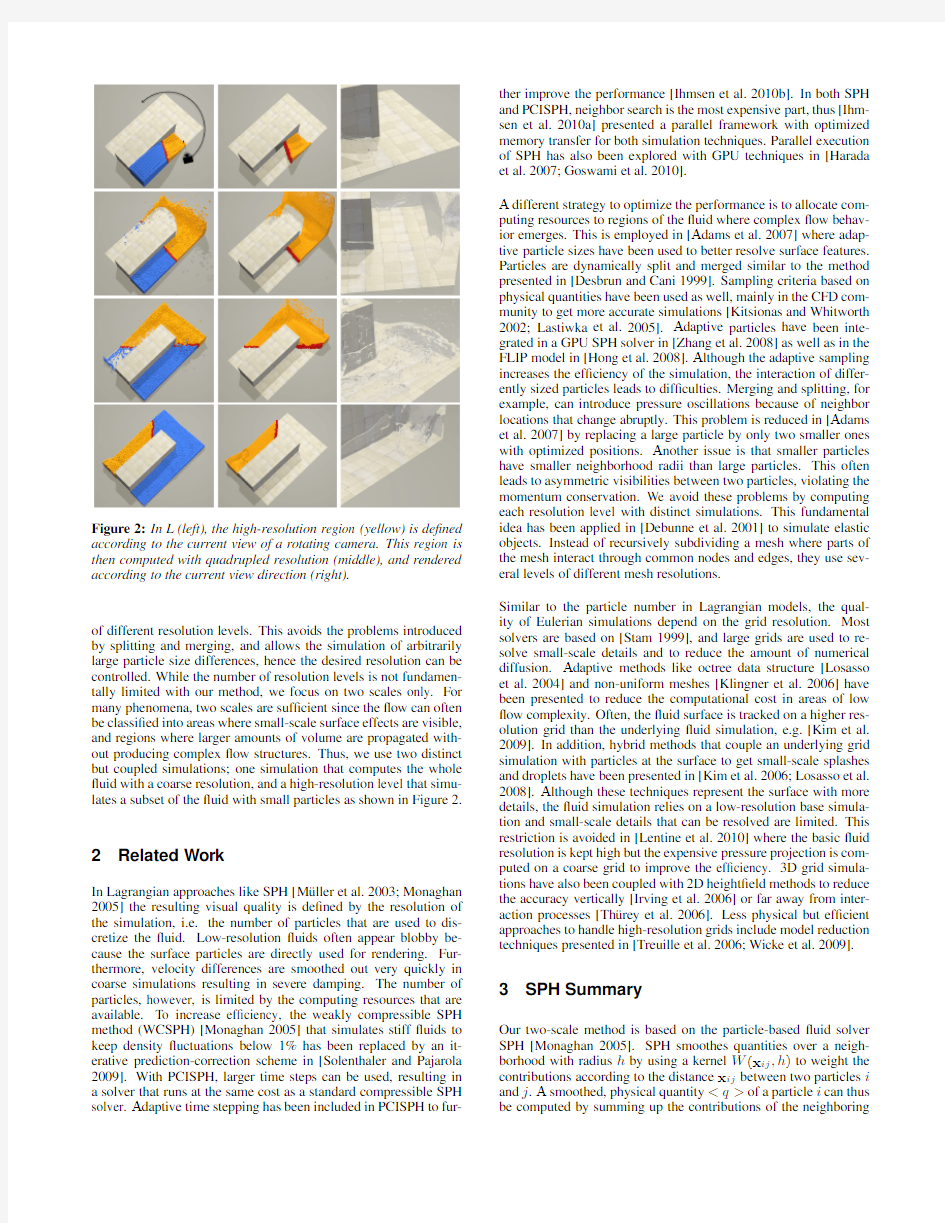
Figure2:In L(left),the high-resolution region(yellow)is de?ned according to the current view of a rotating camera.This region is then computed with quadrupled resolution(middle),and rendered according to the current view direction(right).
of different resolution levels.This avoids the problems introduced by splitting and merging,and allows the simulation of arbitrarily large particle size differences,hence the desired resolution can be controlled.While the number of resolution levels is not fundamen-tally limited with our method,we focus on two scales only.For many phenomena,two scales are suf?cient since the?ow can often be classi?ed into areas where small-scale surface effects are visible, and regions where larger amounts of volume are propagated with-out producing complex?ow structures.Thus,we use two distinct but coupled simulations;one simulation that computes the whole ?uid with a coarse resolution,and a high-resolution level that simu-lates a subset of the?uid with small particles as shown in Figure2. 2Related Work
In Lagrangian approaches like SPH[M¨u ller et al.2003;Monaghan 2005]the resulting visual quality is de?ned by the resolution of the simulation,i.e.the number of particles that are used to dis-cretize the?uid.Low-resolution?uids often appear blobby be-cause the surface particles are directly used for rendering.Fur-thermore,velocity differences are smoothed out very quickly in coarse simulations resulting in severe damping.The number of particles,however,is limited by the computing resources that are available.To increase ef?ciency,the weakly compressible SPH method(WCSPH)[Monaghan2005]that simulates stiff?uids to keep density?uctuations below1%has been replaced by an it-erative prediction-correction scheme in[Solenthaler and Pajarola 2009].With PCISPH,larger time steps can be used,resulting in a solver that runs at the same cost as a standard compressible SPH solver.Adaptive time stepping has been included in PCISPH to fur-ther improve the performance[Ihmsen et al.2010b].In both SPH and PCISPH,neighbor search is the most expensive part,thus[Ihm-sen et al.2010a]presented a parallel framework with optimized memory transfer for both simulation techniques.Parallel execution of SPH has also been explored with GPU techniques in[Harada et al.2007;Goswami et al.2010].
A different strategy to optimize the performance is to allocate com-puting resources to regions of the?uid where complex?ow behav-ior emerges.This is employed in[Adams et al.2007]where adap-tive particle sizes have been used to better resolve surface features. Particles are dynamically split and merged similar to the method presented in[Desbrun and Cani1999].Sampling criteria based on physical quantities have been used as well,mainly in the CFD com-munity to get more accurate simulations[Kitsionas and Whitworth 2002;Lastiwka et al.2005].Adaptive particles have been inte-grated in a GPU SPH solver in[Zhang et al.2008]as well as in the FLIP model in[Hong et al.2008].Although the adaptive sampling increases the ef?ciency of the simulation,the interaction of differ-ently sized particles leads to dif?culties.Merging and splitting,for example,can introduce pressure oscillations because of neighbor locations that change abruptly.This problem is reduced in[Adams et al.2007]by replacing a large particle by only two smaller ones with optimized positions.Another issue is that smaller particles have smaller neighborhood radii than large particles.This often leads to asymmetric visibilities between two particles,violating the momentum conservation.We avoid these problems by computing each resolution level with distinct simulations.This fundamental idea has been applied in[Debunne et al.2001]to simulate elastic objects.Instead of recursively subdividing a mesh where parts of the mesh interact through common nodes and edges,they use sev-eral levels of different mesh resolutions.
Similar to the particle number in Lagrangian models,the qual-ity of Eulerian simulations depend on the grid resolution.Most solvers are based on[Stam1999],and large grids are used to re-solve small-scale details and to reduce the amount of numerical diffusion.Adaptive methods like octree data structure[Losasso et al.2004]and non-uniform meshes[Klingner et al.2006]have been presented to reduce the computational cost in areas of low ?ow complexity.Often,the?uid surface is tracked on a higher res-olution grid than the underlying?uid simulation,e.g.[Kim et al. 2009].In addition,hybrid methods that couple an underlying grid simulation with particles at the surface to get small-scale splashes and droplets have been presented in[Kim et al.2006;Losasso et al. 2008].Although these techniques represent the surface with more details,the?uid simulation relies on a low-resolution base simula-tion and small-scale details that can be resolved are limited.This restriction is avoided in[Lentine et al.2010]where the basic?uid resolution is kept high but the expensive pressure projection is com-puted on a coarse grid to improve the ef?ciency.3D grid simula-tions have also been coupled with2D height?eld methods to reduce the accuracy vertically[Irving et al.2006]or far away from inter-action processes[Th¨u rey et al.2006].Less physical but ef?cient approaches to handle high-resolution grids include model reduction techniques presented in[Treuille et al.2006;Wicke et al.2009].
3SPH Summary
Our two-scale method is based on the particle-based?uid solver SPH[Monaghan2005].SPH smoothes quantities over a neigh-borhood with radius h by using a kernel W(x ij,h)to weight the contributions according to the distance x ij between two particles i and j.A smoothed,physical quantityof a particle i can thus be computed by summing up the contributions of the neighboring
User-defined regions
Low-resolution input Complete neighborhoods Particles added / deleted
Particles advected
Boundary region
L
H
L
H
High-resolution region Feedback
Boundary conditions
Figure 3:Method overview.In our two-scale algorithm,a ?uid subset (yellow particles)determined in the low-resolution level (L)is additionally simulated with higher resolution (H).Appropriate boundary conditions given by L are de?ned (red particles),and a feedback force from H onto L is included to get corresponding ?ows.The particles of both simulations can then be merged for the ?nal rendering.
particles j
=
X j
m j
j q j W (x ij ,h ),(1)
where m j is the mass of particle j and ρj its density.In our im-plementation,we use the SPH force equations for multiple ?uids proposed in [Solenthaler and Pajarola 2008],and the kernels given in [M¨u ller et al.2003].We have additionally integrated our method into the incompressible PCISPH solver presented in [Solenthaler and Pajarola 2009]to keep density variations below 1%.The main difference between SPH /WCSPH and PCISPH is that pressure val-ues are set in a different way:While in SPH /WCSPH pressures are de?ned by the equation of state,PCISPH iteratively adapts pressure values according to the predicted density error of the particles.
4Two-Scale Model
Our method,illustrated in Figure 3,uses two simulations with dif-ferent resolution scales,a low-resolution L and a high-resolution H.The resolution difference is a user-de?ned value and can be cho-sen arbitrarily large.We have de?ned the particle size difference to be a multiple of 8in each scaling step.This results in a regular particle sampling as discussed in Section 4.3.In our simulations we typically use a particle size difference of a factor of 8(doubled reso-lution)or 64(quadrupled resolution).Larger resolution differences can be chosen as well,but,as we discuss in Section 6,our experi-ments have shown that these sizes work best to keep the in?uence of the damping effects from L small.
The coarse level L (blue particles)acts as the base simulation and computes the physics for the whole ?uid.In L we determine a subset of the ?uid that we want to simulate with higher resolution (yellow particles).We show how this region can be determined in Section 4.1.This subset region de?nes the second simulation.An additional particle layer (red particles)is used to model the bound-ary conditions for H.These particles are advected by the ?ow ?eld of L,see Section 4.2,and are dynamically added and deleted as described in Section 4.3.When a boundary particle enters the ac-tive,yellow region,care is taken that the physical quantities change smoothly,see Section 4.4.Since we get more ?ow details in H we include a feedback force from H onto L,this is described in Sec-tion 4.5.The particles of H and L can then be merged for the ?nal rendering.The adapted SPH and PCISPH Algorithm as well as parameter settings are given in Section 5.
4.1High-Resolution Region
The high-resolution region H can be de?ned by any type of sam-pling condition and can change dynamically during the simulation.Since we aim for better visual quality we use geometry driven cri-teria in all our examples,this is insofar important since the surface particles are typically used to reconstruct the ?uid surface.How-ever,physics-driven conditions and combined criteria can be incor-porated as well.
Spatial conditions are straightforward to de?ne,an example is shown in Figure 1where a region around obstacles is de?ned to be simulated with higher resolution to get more surface details at impact locations.Camera information can be additionally included to change the region according to the ?eld of view as shown in Figure 2.Often,it is desirable to allocate computing resources to the surface of the ?uid to get more surface details and ?ne-scaled splashes as in Figure 3.We de?ne a particle to be at the surface if the distance to the center of mass of its neighborhood x i,cm =x i ?P
j x j /P j 1is above a threshold as described in [Solenthaler et al.2007].Isolated particles are detected sepa-rately,they are de?ned by having empty neighborhoods.We use ?ood ?ll to extract several layers of particles that are close to the surface.The interface between multiple ?uids can be determined similarly,the only difference is that x i,cm is based on particles of the same ?uid type only.An example where the interface region is sampled with higher resolution is shown in Figure 4.Our method is able to handle very complex high-resolution regions that dynam-ically change over time,thus any other criterion to de?ne H can be incorporated as well.
In order to keep the computation cost low,as many operations as possible are executed in L.Therefore,the high-resolution region is detected in L and then transferred onto H.Each particle in H stores a parent particle,which is the closest particle in L,and is classi?ed according to the region of its parent.In the following,we refer to the particles that are inside the high-resolution region as active .
4.2Boundary Region
We detect the boundary region analogously to H using the ?ood ?ll method.Boundary particles are advected by the ?ow of L,the velocity is interpolated from L onto H (interpolated quantities q from L are indicated with ?q in the following)by
?v i ∈H =X
k ∈L
v k W,(2)
Figure 4:Our method allows the de?nition of dynamically changing,complex high-resolution regions,like for example the interface between two ?uids with a density ratio of 10.From left to right:In L,the interface is detected and regions are determined.The interface region (yellow)is then computed with doubled resolution.The particle subset of L and the particles of H are combined and rendered.
where W is the box kernel to avoid expensive distance computa-tions.More accurate kernels,for example the SPH density kernel,could be used as well.k ∈L refers to a subset of the neighbors of the parent of i .Since in SPH each particle has 30-40neighbors on average,we de?ne the subset to include all neighbors within a radius of h/2to avoid excessive smoothing.
The computational overhead of boundary particles is small since no physics or neighborhoods have to be computed for them.Nev-ertheless,they are included in the neighborhood of close,active particles and hence contribute to the density and exert viscous and pressure forces.To compute the pair-wise forces,a boundary par-ticle additionally stores the interpolated density and pressure val-ues computed analogously to Equation 2.We have to guarantee that the neighborhood of an active particle close to the boundary region is completely ?lled with particles to avoid imbalanced pres-sure forces.The minimal size of the boundary region is therefore de?ned by the kernel size h as illustrated in Figure 5b).
4.3Dynamic Boundary Particle Generation
When a particle in L enters the boundary region from outside (blue to red)we dynamically create high-resolution boundary par-ticles in H.In case of doubled resolution,8particles with mass m H =m L /8are initialized on a cube around the parent position as illustrated in 2D in Figure 6(a),1).The particle spacing in H is given by d H =d L /r ,where d L is the particle spacing in L and r is the resolution difference factor;in case of doubled resolution the spacing is halved.Our cubical initialization results in a regular particle distribution and is compared to a 2-particles ([Adams et al.2007])and spherical initialization using 7particles ([Desbrun and Cani 1999])in Figure 6(a),2)and 3).Particles created outside the domain (Figure 6(b),i)should not be deleted because this would lead to volume loss.In such situations,we set the particles onto the boundary and slightly shift positions to avoid excessive cluster-ing (Figure 6(b),ii).Since particles undergo a relaxation process to slowly rearrange as soon as they enter the active region (see Sec-tion 4.4),the initial particle con?guration is not too critical regard-ing particle disorder.A boundary particle is deleted as soon as its parent does neither belong to the active nor the boundary region.
4.4Transition Between Boundary and Active
If the parent of a particle j in H leaves the active region and enters the boundary region,the state of j changes as well,hence it is ad-vected by the velocity ?eld of L in the following.The reversed case where a particle j in H enters the active,high-resolution region is critical regarding stability of the simulation.We therefore take care that the physics quantities of a particle j that becomes active
(Fig-
Figure 5:Abrupt density and force changes are avoided during a region transition.This holds for a boundary particle j entering the active region (a),as well as for a
2)
(a)Sampling schemes.i)
(b)Particle creation at walls.
Figure 6:Our method places boundary particles as shown in 1)to get a regular particle distribution.At domain boundaries,parti-cles are set back onto the wall and are slightly shifted (ii)to avoid particle clustering.In this 2D example,orange indicates doubled resolution,and green quadrupled resolution.
ure 5a)as well as the quantities of an active particle i that has j as a neighbor (Figure 5b)do not change from time t to t +1if the particles do not experience any position changes.The latter case is trivially ful?lled;j was already previously included in the computa-tion and thus the density ρi and the pressure force F p i do not change abruptly.The former case is more critical because advection intro-duces errors that could lead to irregular particle sampling.Since the quantities computed with SPH are very sensitive to the number of neighboring particles and their locations,the interpolated quantities at time t do not necessarily correspond to the quantities computed by the physics at t +1.The density,for example,can be much larger than the interpolated value when particles are clustered,leading to large pressure forces.To alleviate this problem,we apply a parti-cle relaxation process that allows the particles to settle into a stable con?guration.The simplest way to achieve this is by letting the physics slowly pushing the particles into the right location.This is done during the time t relax that we have set to 0.05s in all our examples.During this time,the quantities ρj and F p j are computed as follows:
?ρj :We slowly adjust the density to get a smooth transition between ?ρj (t )and ρj (t +1).The density is computed by ρj =αρj +(1?α)?ρj ,where αis set to 0at time t +1and is increased to 1in the following time steps during t relax .
Figure7:A feedback force is included to get corresponding?ow details in L and H.From left to right:L without feedback,L with feedback from H,H.
?F p
j :Pressure forces should slowly push particles away from
each other to get j into a relaxed con?guration.We do that by restricting the velocity magnitude during t relax to?v j=
min(v j,βh
?t ),where?t is the time step,andβis experi-
mentally determined and set to0.05(note the similarity to the Courant condition whereβis typically set between[0.2..0.4]).
?v j is then used to update the position x j+=?t?v j.The ve-locity is set to the interpolated velocity v j=?v j during t relax.
4.5Feedback
The high-resolution simulation H encounters less damping than L and more small-scale details can be resolved,hence the?ows of H and L can diverge.To account for this effect,a feedback force is de?ned to modify the velocity?eld of L according to the?ow of H. The force is computed for each particle i in L marked to be inside the active region by
F feedback
i∈L active =β(v i?
X
j∈H
v j W),(3)
whereβis a constant that de?nes the in?uence of the feedback force.In all our examples,βis set to50based on experiments. j∈H refers to all active particles in H that have i stored as parent. The effect of the feedback force is shown in Figure7.
5Implementation
We have integrated our two-scale method in a standard SPH/WC-SPH solver(Algorithm1and2),as well as in the incompressible PCISPH solver(Algorithm1and3).In both cases,we?rst com-pute the low-resolution physics L with SPH or PCISPH.Then,the different regions are determined,and boundary particles are dy-namically added and deleted in H depending on region changes in L.Physical quantities are interpolated from L onto all bound-ary particles in H as well as all active particles that just left the boundary region.Next,the high-resolution physics is computed. Several time steps are executed depending on the resolution,given by nSubsteps=?t L/?t H.The physics(SPH or PCISPH)is computed for all particles inside the active region,and boundary particles are advected.After each particle is forwarded in time, parents are updated for each particle in H.Since particle locations change only little from one time step to the next,we search the new parent in the neighborhood of the current parent.Only in rare cases where the resulting distance to the parent exceeds h/2(ap-proximately the spacing between the particles in L),the parent is recomputed.Simultaneously to the parent update we transfer the velocity information from H back onto L.This is used in the next time step to compute the feedback forces.
The steps executed in SPH(Algorithm2)correspond to the basic algorithm described in[M¨u ller et al.2003].In PCISPH(Algo-rithm3),it is important that the predicted values of boundary par-ticles are set correctly,they are simply given by v?=?v,ρ?=?ρ,Algorithm1Two-Scales
1while animating do
2compute physics L{SPH or PCISPH}
3determine regions in L
4transfer region information from L onto H
5add/delete H boundary particles
6interpolate quantities from L onto H boundary,activeRelax 7for nSubsteps do
8compute physics H active{SPH or PCISPH}
9advect H boundary
10update parent particle in H
11interpolate feedback infomation from H active onto L Algorithm2Compute Physics SPH(WCSPH)(Particle Set S)
1for all i∈S do
2?nd neighborhoods N i
3for all i∈S do
4computeρi,p i
5for all i∈S do
6compute forces F p,v,g,(feedback)
i
7for all i∈S do
8compute new v i,x i
Algorithm3Compute Physics PCISPH(Particle Set S)
1for all i∈S do
2?nd neighborhoods N i
3for all i∈S do
4compute forces F v,g,(feedback)
i
5while(max(ρerr)?>η)||(iter 6for all i∈S do 7predict v i,x i 8for all i∈S do 9predict densityρ?i 10update pressure p i=f(ρ?i)according to PCISPH 11for all i∈S do 12compute pressure force F p i 13determine max(ρ?err Hactive ) 14for all i∈S do 15compute new v i,x i p=?p.Predicted values of active particles in H that undergo re-laxation get the same restriction as described in Section4.4.Since these particles cannot move freely,a pressure change does not nec-essarily result in the expected change of the particle con?guration and could slow down the convergence of the PCISPH algorithm. We avoid this problem by allowing larger density errors than1% for those particles. In the following,we describe how parameters are set in our im-plementation.First,a particle spacing d L is de?ned,which is the distance between the particles in L.This is used to initialize the particles on a grid.The particle spacing in H,d H,depends on the resolution difference factor r and is given by d H=d L/r;r=2 doubles the resolution.The particle mass m L and m H are then de-?ned by m=d3/ρ0,whereρ0is set to1000.The support radius h is set as twice the particle spacing.During the simulation,this results in30-40neighbors on average.The time step?t L is com-puted with the Courant condition and depends on h,thus?t H is again scaled by r and is given by?t H=?t L/r. 6Results and Discussion Our method can stably handle dynamically changing and complex high-resolution regions.This is shown in Figure4where the inter- 2.0 1.077.21 1.86 5.590.88 2.12 3.6 6.7 3.0 2.4 Table1:Particle number,timings and speed-up factors of our method compared to the single-resolution reference simulation. Table2:Timings[s/time step]for each step of our algorithm. resources to areas of the?uid that are visible to the user.Again, quadrupled resolution is used.In this example,the computational cost is reduced by a factor of3as shown in Table1.Detailed tim-ings for each step of our algorithm are given in Table2,indicating that the overhead of our method is comparatively small.The result is visually compared to the single-scale reference simulation in Fig-ure8,showing that our method produces very similar?ow details. The main difference to the reference solution with1.7M particles is that the?uid movement is slightly damped-this corresponds to the main limitation of our method. This is because the resolution of the base simulation is very coarse in this example(only28k particles), thus L is suffering from damping that is then transferred onto H.In-creasing the base resolution of L or including vorticity con?nement forces to adding back energy could alleviate this problem to some extent.With larger sizes of H,the in?uence of L and thus the damp-ing is reduced,this is shown in Figure10(note that L contains only 16k particles in this example).However,regardless of the size of H, similar surface details emerge.Furthermore,the surface resolution is equivalent to the reference simulation,hence similar rendering quality is achieved.The speed-up factor in this example depends on the size of H and is up to a factor of2.4(see Table1). Another dif?culty with our method is the particle creation at the surface.While our cubical initialization results in a regular particle distribution and keeps horizontal surfaces?at,problems arise with curved surfaces.In such situations,staircase artifacts might be vis-ible,at least until the particles have rearranged due to the physics. Again,this problem can be reduced by slightly increasing the res-olution of L.However,as future work,we would like to explore is compared to the single- ?ood scene.Left:L(without resolution computed with solution. Figure9:The spatial sampling condition(left)can be combined with surface and view information(right)to further reduce the par-ticle number and to reach a larger speed-up. the inclusion of surface normals in the particle creation process to avoid the dependency on the resolution of L. In SPH,the computational costs increase linearly with the number of particles.Thus,the optimal speed-up of a multi-scale method is linear to the reduction rate of the particle number,e.g.if the particle number is halved,the frame rate is optimally doubled.Our results show that our method features this characteristics and furthermore indicate that the achieved speed-up factor highly depends on the particular scene set-up and the sampling criterion that is used. The presented timings are all measured on a22.66GHz Quad-Core Intel machine.Our code can be optimized by integrating more sophisticated techniques for neighbor search presented in[Ihmsen et al.2010a]and adaptive time stepping[Ihmsen et al.2010b].We used PCISPH to compute the examples in Figure1and10,and SPH for all other simulations.While we focused on two resolution scales only,our method can be extended in a straightforward way to han-dle multiple scales.However,for most applications,it is suf?cient Figure10:Similar surface features emerge with different sizes of H.The size of H affects the damping in?uence of L,the particle resolution at the surface however is equivalent. to classify the?uid into regions where small-scale surface details and splashes emerge,and areas of low?ow complexity. 7Conclusion We have presented a two-scale method for particle-based?uids in order to reduce the overall computational cost while still achiev-ing small-scale surface details comparable to the single-resolution simulation.Our method is based on the idea to simulate distinct particle sizes in individual but coupled simulations.The coupling is done by introducing appropriate boundary conditions as well as feedback forces.Dynamic particle generation and deletion as well as stable transitions between the regions enable changing and com-plex high-resolution areas.Our method can be easily integrated into an existing particle solver to improve the computational ef?ciency. Moreover,it allows the allocation of computational resources to those parts of the?uid where a higher resolution is desirable. References A DAMS,B.,P AULY,M.,K EISER,R.,AND G UIBAS,L.J.2007. Adaptively sampled particle?uids.ACM Trans.Graph.(SIG-GRAPH Proc.)26,3,48–54. D EBUNNE,G.,D ESBRUN,M.,C ANI,M.-P.,AND B ARR,A.H. 2001.Dynamic real-time deformations using space and time adaptive sampling.In Proc.of ACM SIGGRAPH2001,31–36. D ESBRUN,M.,AND C ANI,M.P.1999.Space-time adaptive simulation of highly deformable substances.Tech.rep.,INRIA Nr.3829. G OSWAMI,P.,S CHLEGEL,P.,S OLENTHALER, B.,AND P A- JAROLA,R.2010.Interactive SPH simulation and rendering on the GPU.In Proc.of the ACM SIGGRAPH/Eurographics Symposium on Computer Animation,55–64. H ARADA,T.,K OSHIZUKA,S.,AND K AWAGUCHI,Y.2007. Smoothed Particle Hydrodynamics on GPUs.In Proc.of Com-puter Graphics International,63–70. H ONG,W.,H OUSE,D.H.,AND K EYSER,J.2008.Adaptive particles for incompressible?uid https://www.360docs.net/doc/cf7272778.html,put.24, 535–543. I HMSEN,M.,A KINCI,N.,B ECKER,M.,AND T ESCHNER,M. 2010.A parallel SPH implementation on multi-core https://www.360docs.net/doc/cf7272778.html,-puter Graphics Forum30,1,99–112. I HMSEN,M.,A KINCI,N.,G ISSLER,M.,AND T ESCHNER, M.2010.Boundary handling and adaptive time-stepping for PCISPH.In Proc.of VRIPHYS,79–88. I RVING,G.,G UENDELMAN,E.,L OSASSO,F.,AND F EDKIW,R. 2006.Ef?cient simulation of large bodies of water by coupling two and three dimensional techniques.ACM Trans.Graph.(SIG-GRAPH Proc.)25,805–811.K IM,J.,C HA,D.,C HANG,B.,K OO,B.,AND I HM,I.2006. Practical animation of turbulent splashing water.In Proc.of the ACM SIGGRAPH/Eurographics Symposium on Computer Ani-mation,335–344. K IM,D.,S ONG,O.-Y.,AND K O,H.-S.2009.Stretching and wiggling liquids.ACM Trans.Graph.(SIGGRAPH ASIA Proc.) 28,5,1–7. K ITSIONAS,S.,AND W HITWORTH,A.2002.Smoothed Particle Hydrodynamics with particle splitting,applied to self-gravitating collapse.MNRAS330,1,129–136. K LINGNER,B.M.,F ELDMAN,B.E.,C HENTANEZ,N.,AND O’B RIEN,J.F.2006.Fluid animation with dynamic meshes. ACM Trans.Graph.(SIGGRAPH Proc.)25,820–825. L ASTIWKA,M.,Q UINLAN,N.,AND B ASA,M.2005.Adaptive particle distribution for Smoothed Particle Hydrodynamics.Int. J.Numer.Meth.Fluids47,1403–1409. L ENTINE,M.,Z HENG,W.,AND F EDKIW,R.2010.A novel algorithm for incompressible?ow using only a coarse grid pro-jection.ACM Trans.Graph.(SIGGRAPH Proc.)29,4,1–9. L OSASSO,F.,G IBOU,F.,AND F EDKIW,R.2004.Simulating wa-ter and smoke with an octree data structure.ACM Trans.Graph. (SIGGRAPH Proc.)23,3,457–462. L OSASSO,F.,T ALTON,J.,K WATRA,J.,AND F EDKIW,R.2008. Two-way coupled SPH and particle level set?uid simulation. IEEE TVCG14,4,797–804. M ONAGHAN,J.J.2005.Smoothed Particle Hydrodynamics.Rep. Prog.Phys.68,1703–1759. M¨ULLER,M.,C HARYPAR,D.,AND G ROSS,M.2003.Particle-based?uid simulation for interactive applications.In Proc.of the ACM SIGGRAPH/Eurographics Symposium on Computer Ani-mation,154–159. S OLENTHALER,B.,AND P AJAROLA,R.2008.Density contrast SPH interfaces.In Proc.of the ACM SIGGRAPH/Eurographics Symposium on Computer Animation,211–218. S OLENTHALER, B.,AND P AJAROLA,R.2009.Predictive-corrective incompressible SPH.ACM Trans.Graph.(SIG-GRAPH Proc.)28,3,1–6. S OLENTHALER,B.,Z HANG,Y.,AND P AJAROLA,R.2007.Ef-?cient re?nement of dynamic point data.In Proc.of the Euro-graphics Symposium on Point-Based Graphics,65–72. S TAM,J.1999.Stable?uids.In Proc.of SIGGRAPH99,121–128. T H¨UREY,N.,R¨UDE,U.,AND S TAMMINGER,M.2006.Anima-tion of open water phenomena with coupled shallow water and free surface simulation.Proc.of the Eurographics/ACM SIG-GRAPH Symposium on Computer Animation,157–166. T REUILLE,A.,L EWIS,A.,AND P OPOVI′C,Z.2006.Model re-duction for real-time?uids.ACM Trans.Graph.(SIGGRAPH Proc.)25,826–834. W ICKE,M.,S TANTON,M.,AND T REUILLE,A.2009.Modu-lar bases for?uid dynamics.ACM Trans.Graph.(SIGGRAPH Proc.)28,3,1–8. Z HANG,Y.,S OLENTHALER,B.,AND P AJAROLA,R.2008.Adap-tive sampling and rendering of?uids on the GPU.In Proc.of the Eurographics Symposium on Volume and Point-Based Graphics, 137–146.