Vertex Collocation Profiles Subgraph Counting for Link Analysis and Prediction

Vertex Collocation Pro?les:Subgraph Counting for Link

Analysis and Prediction

Ryan N.Lichtenwalter University of Notre Dame Notre Dame,Indiana,USA rlichten@https://www.360docs.net/doc/d018613984.html,

Nitesh V.Chawla University of Notre Dame Notre Dame,Indiana,USA nchawla@https://www.360docs.net/doc/d018613984.html,

ABSTRACT

We introduce the concept of a vertex collocation pro?le (VCP)for the purpose of topological link analysis and pre-diction.VCPs provide nearly complete information about the surrounding local structure of embedded vertex pairs. The VCP approach o?ers a new tool for domain experts to understand the underlying growth mechanisms in their networks and to analyze link formation mechanisms in the appropriate sociological,biological,physical,or other con-text.The same resolution that gives VCP its analytical power also enables it to perform well when used in super-vised models to discriminate potential new links.We?rst develop the theory,mathematics,and algorithms underly-ing VCPs.Then we demonstrate VCP methods performing link prediction competitively with unsupervised and super-vised methods across several di?erent network families.We conclude with timing results that introduce the comparative performance of several existing algorithms and the practica-bility of VCP computations on large networks. Categories and Subject Descriptors

H.2.8[Database Management]:Database Applications—Data mining

Keywords

graph theory,link analysis,link prediction,network analysis 1.INTRODUCTION

Link prediction is the task of inferring links in a graph G t+1based on the observation of a graph G t.It may be that t+1follows t in time,or it may be that t+1represents some other evolution or manipulation of the graph such as including additional links from experiments that are di?-cult or expensive to conduct.Link prediction stated in this manner is a binary classi?cation problem in which links that form construct the positive class and links that do not form construct the negative class.Link analysis,more loosely de-?ned,is the problem of identifying evolutionary processes or growth mechanisms in a network that are responsible for the formation of new relationships between nodes.

We formally de?ne a new technique for performing both link prediction and link analysis based on a restrictive rep-resentation of the local topological embedding of the source Copyright is held by the International World Wide Web Conference Com-mittee(IW3C2).Distribution of these papers is limited to classroom use, and personal use by others.

WWW2012,April16–20,2012,Lyon,France.

ACM978-1-4503-1229-5/12/04.and target vertices.This idea is a generalization and exten-

sion of the triangle counting approach for multi-relational prediction in[6].It also draws on concepts from literature on graphlets as introduced in[19]and to a lesser degree from motif analysis as discussed in[17].

Many existing link prediction models compress a selection of simple information in theoretically or empirically guided ways.By contrast the VCP approach preserves as much topological information as possible about the embedding of the source and target vertices.It also extends naturally to multi-relational networks and can thereby encode a variety of additional information such as edge directionality.It can encode continuous quantities such as edge weights by bin-ning into relational categories,such as high activity and low https://www.360docs.net/doc/d018613984.html,rmation about the nature of relationships is maintained as structures are identi?ed within the network. We proceed with a formal exploration of VCP,discuss its re-lationship to isomorphism classes,provide algorithms that formally describe VCP computations,and demonstrate the potential of VCP in link prediction and analysis as well as feasibility in terms of computational time.Fast forms of the algorithms listed within this paper are all implemented in C++and integrated into the LPmade[14]link prediction software and are thus freely available on MLOSS.

2.VERTEX COLLOCATION PROFILES Formally,a vertex collocation pro?le(VCP),written as VCP n,r

i,j

,is a vector describing the relationship between two vertices,v i and v j,in terms of their common membership in all possible subgraphs of n vertices over r relations.A VCP

element,VCP n,r

i,j

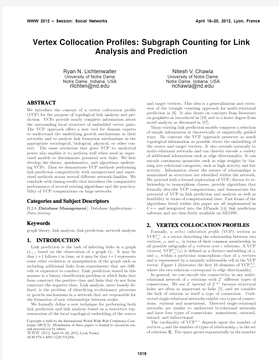
(x)is de?ned as a distinct embedding of v i and v j within a particular isomorphism class of n vertices and is represented by a uniquely addressable cell in the VCP vector.Figure1illustrates the?rst16elements of VCP3,2s,t, where the two relations correspond to edge directionality. In general,we can encode the connectivity in any multi-relational network of r relations with2r di?erent types of connections.We use2r instead of2r?1because structural holes are often as important as links[5],and we consider the lack of relation as itself a type of connection.Undi-rected single-relational networks exhibit two types of connec-tions:existent and nonexistent.Directed single-relational networks are similar to undirected bi-relational networks and have four types of connections:nonexistent,outward, inward,and bidirectional.

The cardinality of VCP n,r depends upon the number of vertices n and the number of types of relationship r in the set of relations R.The space grows exponentially in the number

Figure1:Elements of VCP3,2s,t.16through31are

identical except with the presence of e t,s.

H

H

H

H H

n

r

1234

34322562048

43220481310728.4×106

55125242885.4×1085.5×1011

6163845.4×1081.8×10135.8×1018

Table1:Number of enumerated subgraphs compos-

ing VCP for values of n and r.

of vertices with the base as the cardinality of the power

set of relations.The formula for the number of subgraphs

is written in intuitive form in Equation1.The multiplier

accounts for the number of possible collocation structures

disregarding any links between the source and the target.

The multiplicand is the number of di?erent ways two vertices

with the same embedding can appear based on the di?erent

link possibilities between them.

(2r)

n(n?1)2?1

×2r?1(1)

We can manipulate these to achieve the simpler formula

below.

2n(n?1)r

2

?1(2)

Table1illustrates the number of subgraphs respecting

vertex identity that compose the VCP given di?erent values

of n and r.

The number of subgraphs grows at such a rate as to make

the sheer size of output unmanageable for large values of n

and r.The rate of growth of

VCPs is much

slower due

to

superlinear increases in

the isomorphisms with increasing n,

but nonetheless VCP cardinality

also grows quickly.Fortu-

nately,the most important information is typically located

close to the source and target vertices,and many networks

have few types of relationships.When the number of rela-

tionship types is high,relationships can be compressed or

discarded in various ways albeit with a loss of information.

2.1Isomorphisms

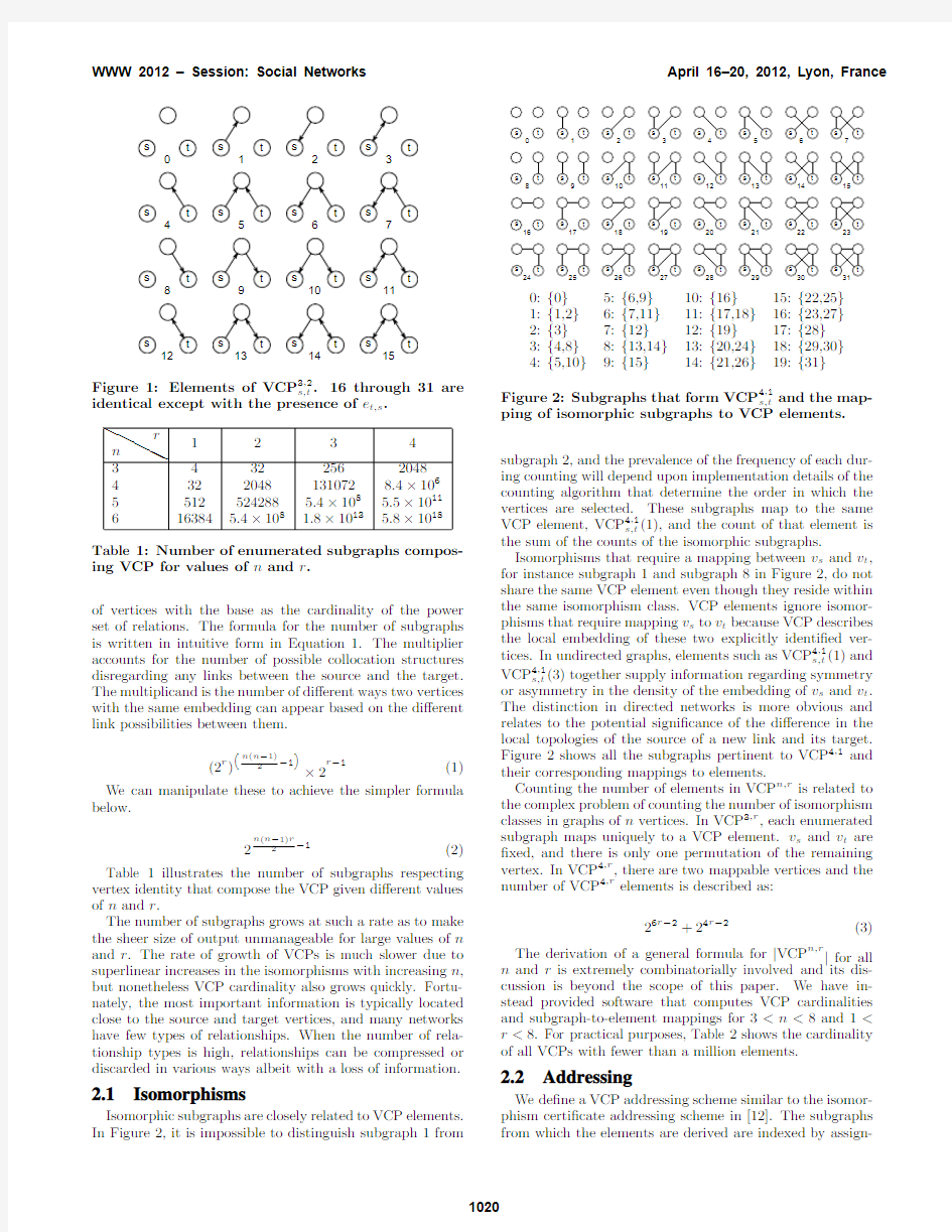
Isomorphic subgraphs are closely related to VCP elements.

In Figure

2,it is impossible to distinguish subgraph1from

0:{0}5:{6,9}10:{16}15:{22,25}

1:{1,2}6:{7,11}11:{17,18}16:{23,27}

2:{3}7:{12}12:{19}17:{28}

3:{4,8}8:{13,14}13:{20,24}18:{29,30}

4:{5,10}9:{15}14:{21,26}19:{31}

Figure2:Subgraphs that form VCP4,1s,t and the map-

ping of isomorphic subgraphs to VCP elements.

subgraph2,and the prevalence of the frequency of each dur-

ing counting will depend upon implementation details of the

counting algorithm that determine the order in which the

vertices are selected.These subgraphs map to the same

VCP element,VCP4,1s,t(1),and the count of that element is

the sum of the counts of the isomorphic subgraphs.

Isomorphisms that require a mapping between v s and v t,

for instance subgraph1and subgraph8in Figure2,do not

share the same VCP element even though they reside within

the same isomorphism class.VCP elements ignore isomor-

phisms that require mapping v s to v t because VCP describes

the local embedding of these two explicitly identi?ed ver-

tices.In undirected graphs,elements such as VCP4,1s,t(1)and

VCP4,1s,t(3)together supply information regarding symmetry

or asymmetry in the density of the embedding of v s and v t.

The distinction in directed networks is more obvious and

relates to the potential signi?cance of the di?erence in the

local topologies of the source of a new link and its target.

Figure2shows all the subgraphs pertinent to VCP4,1and

their corresponding mappings to elements.

Counting the number of elements in VCP n,r is related to

the complex problem of counting the number of isomorphism

classes in graphs of n vertices.In VCP3,r,each enumerated

subgraph maps uniquely to a VCP element.v s and v t are

?xed,and there is only one permutation of the remaining

vertex.In VCP4,r,there are two mappable vertices and the

number of VCP4,r elements is described as:

26r?2+24r?2(3)

The derivation of a general formula for|VCP n,r|for all

n and r is extremely combinatorially involved and its dis-

cussion is beyond the scope of this paper.We have in-

stead provided software that computes VCP cardinalities

and subgraph-to-element mappings for3

r<8.For practical purposes,Table2shows the cardinality

of all VCPs with fewer than a million elements.

2.2Addressing

We de?ne a VCP addressing scheme similar to the isomor-

phism certi?cate addressing scheme in[12].The subgraphs

from which the elements are derived are indexed by assign-

Table 2:Number of elements in VCP n,r i,j .

H H H H H n r

1234

53432256204816384

420108866560--512091520---6996----712208---

-

ing powers of 2r to edges in the adjacency matrix in increas-ing lexicographical order starting with e 1,3and ending with e n ?1,n .v s and v t are de?ned as v 1and v 2respectively,and e 1,2is the edge of highest value.The value of each edge is multiplied by the index of the lexicographically ordered power set,P (R ),corresponding to the ordered set of R rela-tions on the edge.Figures 1and 2demonstrate the indexing scheme for two di?erent values of n and r .For any selec-tion of vertices v s ,v t ,v 3,...,v n ,this addressing scheme will map the resulting multi-relational subgraph to an index that exists within a set of indices of isomorphic structures.

We de?ne the unique address of a VCP element as the subgraph representative with the lowest index within the corresponding isomorphism class.This addressing scheme provides a unique address for all elements in all VCPs.The addresses for elements in VCP 4,1are provided in Figure 2.Because manual identi?cation of isomorphism classes is error-prone and di?cult especially as the number of sub-graphs increases,we have provided a program that outputs the mapping from all subgraph indices to their correspond-ing element addresses for all VCPs.

2.3Directionality

Directed networks with r relations can be treated simi-larly to undirected networks with 2r relations with one ma-jor caveat.The subgraph-to-element mapping di?ers with directed networks.Taking e x i,j momentarily as notation for an edge of relation x and 2x as relation x in the opposite

direction,e x i,j ≡e x

j,i in undirected multi-relational networks,

but e x i,j ≡e 2x

j,i in directed networks.In the context of larger subgraphs,this causes more isomorphic equivalences and de-creases the cardinality of the VCP by comparison to its undirected pseudo-equivalent,a fact demonstrated in Fig-ure 3.For instance,VCP 4,

2contains 1088elements

whereas the

directed variant of VCP 4,1contains only 1056elements.

≡

≡

Figure 3:Subgraphs from undirected VCP 4,2and di-rected VCP 4,1.The directed subgraphs both map to directed VCP 4,1(221),but the undirected subgraphs map to two di?erent VCP 4,2elements.

Algorithm 1VCP 3,r

Input:network G =(V,E ),

relations R ,i :v i ∈V ,j :v j ∈V

Output:V CP 3,|R|

i,j 1:σi,j ←Φ(P (R ),e i,j )

2:for k :e i,k ∈E i ∧e j,k ∈E j do 3:σi,k ←Φ(P (R ),e i,k )4:σj,k ←Φ(P (R ),e j,k )

5:λ←22|R|σi,j +2|R|σj,k +σi,k

6:V CP 3,|R|i,j [λ]←V CP 3,|R|

i,j [λ]+17:end for

8:for k :e i,k ∈E i ∧e j,k /∈E j do 9:σi,k ←Φ(P (R ),e i,k )

10:λ←22|R|σi,j +2|R|σj,k +σi,k

11:V CP 3,|R|i,j [λ]←V CP 3,|R|

i,j [λ]+112:end for

13:for k :e i,k /∈E i ∧e j,k ∈E j do 14:σj,k ←Φ(P (R ),e j,k )

15:λ←22|R|σi,j +2|R|σj,k +σi,k

16:V CP 3,|R|i,j [λ]←V CP 3,|R|

i,j [λ]+117:end for

18:λ←22|R|σi,j 19:for k :e i,k /∈E i ∧e j,k /∈E j do

20:V CP 3,|R|i,j [λ]←V CP 3,|R|

i,j [λ]+121:end for

22:

return V CP 3,|R|

i,j

Therefore,the algorithms in Section 3and the procedures described by all provided code work with only minor ad-justments,which are essentially related to the subgraph-to-element mapping.We include software to construct the mapping for VCP 4,1where there are actually two relations corresponding to directionality.

3.ALGORITHMS

Algorithms 1and 2serve as reference algorithms and not as optimized or even asymptotically optimal approaches for VCP element counting.In fact,implementations of the na ¨?ve VCP 4,1algorithm fail to return within a reasonable time for networks with even thousands of nodes.Fortu-nately,it is possible to design much faster approaches,and we implemented these approaches and provide them as a set of C++?les.We also present a more innovative algorithm,Algorithm 3for counting VCP 4,1that corresponds to the approach in the code for that VCP.

3.13-Vertex VCP

Algorithm 1demonstrates how to calculate VCP 3,r for the set of r relations in R .Φ(P (R ),e x,y )refers to a procedure to determine the index of the multi-relational edge e x,y in P (R ),the lexicographically ordered power set of relations.This procedure can derive power set indices e?ciently by setting individual bits in the index according to the presence of the relation corresponding to that bit and indexing the bits by the natural order of the relations themselves.This na ¨?ve algorithm ?rst determines the contribution of any edge types between v i and v j ,the ?xed source and tar-

get vertices for the link.Then it counts subgraphs with a third vertex connected to both v i and v j,subgraphs only connected to v i,subgraphs only connected to v j,and both.σrepresents the identity of an edge within P(R)andλrep-resents the index of the subgraph.Because no isomorphisms exist with only one mappable vertex,the algorithm directly increments the VCP elements corresponding to the under-lying subgraph index as contrasted to Algorithm2wherein the subgraph index must be mapped to an element address.

A na¨?ve implementation iterates through each vertex in the network and determines the corresponding subgraph in-dex by summing the edge contributions.For one free vertex, this approach has complexity O |V|log |E||V| per edge output assuming O log |E||V| neighbor search time for the average case.This complexity is probably feasible for small networks,but may require an unacceptably long time for large networks.It is simple to improve upon this ap-proach by considering only the vertices that are neighbors, denoted byΓ(v x)of v i,v j,both,or neither and perform-ing set operations.VCP3,1i,j(0)is populated by subtracting |Γ(v i)∪Γ(v j)|from|V|?2.VCP3,1i,j(1)and VCP3,1i,j(2)are populated by computing set di?erences|Γ(v i)?Γ(v j)|and |Γ(v j)?Γ(v i)|respectively.VCP i,j is computed as the inter-section|Γ(v i)∩Γ(v j)|.These operations can be performed quickly especially in graphs in which adjacencies are repre-sented as ordered lists of neighbors.This implementation has average-case complexity O |E||V| per edge output.

3.24-Vertex VCP

Algorithm2iterates through every pair of free vertices, yielding a complexity of O |V|2log |E||V| from |V|?22 pairs of free vertices.This requires trillions of operations even for small networks.It is possible to reduce this time greatly by restricting consideration to known neighbors as described in the discussion of Algorithm1,but na¨?ve im-plementations of this optimization involve many expensive operations in hashes or balanced search trees.

Algorithm3instead uses a minimal number of set op-erations implemented as merge operations on ordered lists. Figure4provides an illustration of the sets mentioned in the following explanation.First,the number of connected pairs and unconnected pairs is computed once for the en-tire network,and these values are represented asχG and?G respectively.We must also track the connected pairs and unconnected pairs internal to the vertices in our consider-ation for the prediction output to di?erentiate VCP4,1(0) from VCP4,1(10).We start by constructing a set of po-tential“third position”vertices,Γ3,asΓ(v i)∩Γ(v j).For each member ofΓ3,we construct two disjoint sets of“fourth position”vertices,Γ4containing vertices reachable by our current member ofΓ3but not contained withinΓ3,andΓ4a constructed fromΓ3excluding the current member ofΓ3. InΓ4,we count new connections and gaps in the con?gu-ration,and we increment the counter for the corresponding subgraph.ForΓ4a,we do not count connections and gaps since con?gurations using those set members are counted when they serve as members ofΓ3,or“third position”ver-tices.Likewise,we only count subgraphs with two mem-bers fromΓ3when the member fromΓ4a compares lower. This avoids multi-counting.After considering the con?g-urations from all members ofΓ4andΓ4a,we account for Algorithm2VCP4,1(Simple)

Input:network G=(V,E),

i:v i∈V,

j:v j∈V,

subgraph-element mapping M

Output:V CP4,1

i,j

1:for k:v k=v i∧v k=v j do

2:for l:v l=v i∧v l=v j∧l>k do

3:λ←0

4:if e i,k∈E then

5:λ←λ+1

6:end if

7:if e i,l∈E then

8:λ←λ+2

9:end if

10:if e j,k∈E then

11:λ←λ+4

12:end if

13:if e j,l∈E then

14:λ←λ+8

15:end if

16:if e k,l∈E then

17:λ←λ+16

18:end if

19:V CP4,1

i,j

(M(λ))←V CP4,1

i,j

(M(λ))+1

20:end for

21:end for

22:return V CP4,1

i,j

structures with isolates by contributing|V|?2?|Γ3|?|Γ4|

to V CP4,1

i,j

(M(λ1)).We also account for multi-counting of VCP4,1(0)due to duplicate consideration of gaps by sub-

tracting the same quantity from V CP4,1

i,j

(M(0)).Finally, we compute VCP4,1(0)and VCP4,1(10)using our computa-tions of vertices and gaps in the vertices we have encountered in the singleΓ3and multipleΓ4sets and subtract their con-tributions from the contributions from the entire network. It is possible to perform the entire procedure using a few relatively inexpensive merge operations in ordered vectors or lists and entirely avoiding hashes or balanced trees.This exposition mostly describes the procedure to quickly com-pute VCP4,1albeit omitting minor implementation details. We refer more interested readers to the code itself.

3.3Extension to Complex Networks

It is trivial to extend VCP algorithms to networks more complex than those on which we obtained our results.This includes any form of edge feature such as directionality, weight,temporality,di?erent relation types,or any infor-mation describing edges or vertex pairs that either exists categorically or can be quantized.One amenable network representation associates an ordered set of bits with each edge.Each bit corresponds to the presence of a particular relation or some Boolean descriptor for a pair of vertices. The determination of the existence of an edge for single-relational data instead becomes an evaluation of the edge as the binary-coded integral value of the ordered set of bits. This is one conceivable implementation forΦ(P(R),e x,y)in Algorithm1,which replaces the constant values for allλupdates in Algorithms2and3.For most values of r,this

Algorithm3VCP4,1(Fast) Input:network G=(V,E),

i:v i∈V,

j:v j∈V,

subgraph-element mapping M

count of connected pairsχG,

count of unconnected pairs?G Output:V CP4,1

i,j

1:υ←2

2:χ←0

3:?←0

4:Γ3←Γ(v i)∩Γ(v j)

5:for k:v k∈Γ3do

6:λ1←0

7:if e i,k∈E∨e k,i∈E then 8:λ1←λ1+1

9:χ←χ+1

10:else

11:?←?+1

12:end if

13:Γ4←Γ(v k)?Γ3

14:υ←υ+|Γ4|

15:for l:v l∈Γ4do

16:λ2←λ1

17:if e i,l∈E∨e l,i∈E then 18:λ2←λ2+2

19:χ←χ+1

20:else

21:?←?+1

22:end if

23:if e j,l∈E∨e l,j∈E then 24:λ2←λ2+8

25:χ←χ+1

26:else

27:?←?+1

28:end if

29:if e k,l∈E∨e l,k∈E then 30:λ2←λ2+16

31:χ←χ+1

32:else

33:?←?+1

34:end if 35:V CP4,1

i,j (M(λ2))←V CP4,1

i,j

(M(λ2))+1

36:end for

37:for l:v l∈Γ3∧l>k do 38:λ2←λ1

39:if e i,l∈E∨e l,i∈E then 40:λ2←λ2+2

41:end if

42:if e j,l∈E∨e l,j∈E then 43:λ2←λ2+8

44:end if

45:if e k,l∈E∨e l,k∈E then 46:λ2←λ2+16

47:χ←χ+1

48:else

49:?←?+1

50:end if 51:V CP4,1

i,j (M(λ2))←V CP4,1

i,j

(M(λ2))+1

52:end for

53:ζ←|Γ3|+|Γ4|

54:V CP4,1

i,j (M(λ1))←V CP4,1

i,j

(M(λ1))+|V|?2?ζ

55:V CP4,1

i,j (M(0))←V CP4,1

i,j

(M(0))+|V|?2?ζ

56:end for

57:ρ←e i,j∈E∨e j,i∈E

58:V CP4,1

i,j (M(16))←V CP4,1

i,j

(M(16))+χG?(χ+ρ)

59:V CP4,1

i,j (M(0))←V CP4,1

i,j

(M(0))+?G?(?+?(ρ))?(2|V|?υ)

60:return V CP4,1

i,j

Figure4:A depiction of the sets considered within Algorithm3.

can be implemented as a constant-time operation equivalent to retrieving the value of a variable,so the asymptotic cost of populating the VCP vector is una?ected.Excepting the additional costs of writing output and of allocating and deal-locating the storage necessary to hold the additional multi-relational structural elements,which is inexpensively pro-portional to2r,the computational complexity of the multi-relational extension is no greater than for single-relational networks.

4.RESULTS

First,we illustrate how VCP can serve as a powerful link analysis and modeling tool.Then we perform a standard comparison of the link prediction e?cacy of VCP and a se-lection of other methods.Timing results are rarely provided in link prediction work despite vast di?erences in the run-ning time and feasibility of methods.For this reason and because we believe many might suspect that a completely theoretically aligned implementation of VCP is computa-tionally unachievable,we also provide comparative timing results.

4.1Data

We present results for several di?erent data sets to demon-strate the performance of the techniques under compari-son for di?erent families of networks.Though all of these data sets contain information with which to generate edge weights,we are interested in providing purely structural comparison here,so all quantitative results are presented based on networks constructed without edge weights.

calls is a stream of262million cellular phone calls from a major cellular phone service provider.We construct directed networks from the calls by creating a node v i for each caller and a directed link e i,j from v i to v j if and only if v i calls v j. sms is a stream of84million text messages from the same source as calls and constructed in the same manner.These two data sets are not publicly available.

condmat-collab is a stream of19,464multi-agent events representing condensed matter physics collaborations from 1995to2000.We construct undirected networks from the collaborations by creating a node for each author in the event and an undirected link connecting each pair of au-thors.For all experiments involving condmat,we use the years1995to1999for constructing training data and the year2000for testing.

dblp-cite is a citation network based on the DBLP com-puter science bibliography.Each researcher is a node v i and directed networks are formed by viewing a citation by re-searcher v i of work by researcher v j as a directed link e i,j. The dblp-collab network uses the same raw data,but links are based on co-authorship collaborations.An undirected

Table3:Some basic properties of the data sets.These?gures are reported for networks constructed using all available longitudinal data.C represents average clustering coe?cient and r a represents assortativity coe?cient.

Name Directed Vertices Edges C r a

calls 7,786,47133,292,5080.1270.212

condmat-collab17,216110,5440.6420.177

dblp-cite 15,963344,3730.128-0.046

dblp-collab367,7252,088,7100.6170.254

disease-g39915,6340.665-0.310

disease-p43781,1580.818-0.406

hepth-cite 8,249335,0280.3520.097

hepth-collab8,38140,7360.4660.237

huddle4,243997,0080.591-0.211

patents-collab1,162,2275,448,1680.5310.141

sms 5,016,74611,598,8430.0480.042

link exists between v i and v j if both are an author on the same paper.

disease-g is a network in which nodes represent diseases and the links between diseases represent the co-occurrence of particular genotypic characteristics.Links are undirected. This network is not longitudinal,but?nding unobserved links is an important task,so we have no choice but to esti-mate performance by randomly removing links to construct test sets.disease-p is from the same source as disease-g. The di?erence is that the links in disease-p represent the co-occurrence of phenotypic characteristics.Predictions of common expressions between diseases are uninteresting since expressions are either observed between diseases or they are not,so practically speaking the value of phenotypic pre-dictions is negligible.Nonetheless,holding out phenotypic links and subsequently predicting their presence is equally instructive for the purposes of predictor evaluation.

hepth-cite and hepth-collab are formed in exactly the same way as dblp-cite and dblp-collab respectively.The raw data for these networks is a set of publications in the-oretical high-energy physics.In particular,we used a data set post-processed by the Knowledge Discovery Lab at the University of Massachusetts for use in[16]rather than the original2003KDD Cup competition data set.This form of the data set o?ers advantages in data quality and entity consolidation and disambiguation.

The huddle data set from[20]is transaction data gath-ered at a convenience store on the University of Notre Dame campus.The data was collected from June2004to Febru-ary2007.Products are represented by nodes,and products purchased together in the same transaction are represented by undirected links.

The patents-collab data set is constructed from the data at the National Bureau of Economic Research.Nodes rep-resent authors of patents and undirected links are formed between authors who work together on the same patent. 4.2Experimental Setup

To run our experiments,we integrated VCP with the LP-made link prediction software[14].LPmade uses a GNU make architecture to automate the steps necessary to per-form supervised link prediction.This integration will allow those interested in VCP for link prediction and other pur-poses to test it on their networks easily.

We compare link prediction output against representatives from di?erent predictor families established as strong by pre-vailing literature[13].The unsupervised selections include the Adamic/Adar common neighbors predictor[1],the Katz path-based predictor[11],and the preferential attachment model[2,18].We also compare against the HPLP super-vised link prediction framework contributed by[15]includ-ing the PropFlow feature.HPLP combines simple topologi-cal information such as node degree and common link predic-tors into a bagged random forests classi?cation framework with undersampling,a framework that the authors showed works well.

When performing classi?cation using VCPs,we opted for the bagged[3]random subspaces[9]implementation from WEKA3.5[22].This classi?cation scheme o?ers signi?-cantly lower peak memory requirements than random forests while simultaneously providing the potential to handle fea-ture redundancy[9].We considered presenting results with HPLP also using random subspaces,but we determined that random subspaces produced decreased or comparable per-formance to the original reference implementation,so we present HPLP results unmodi?ed using random forests[4]. We used the default values from HPLP of10bags of10 random forest trees,10bags of10random subspaces for VCP classi?ers,and training set undersampling to25%pos-itive class prevalence in training.We did not change the size or distribution of the testing data.For undirected networks, we resolve f(v s,v t)=f(v t,v s),by computing the arith-metic mean to serve as the?nal prediction output.By de-fault,LPmade includes features that consider edge weights such as the sum of incoming and outgoing link weights,and PropFlow inherently considers edge weights.We are inter-ested in the comparative prediction performance of the link structure alone,so we ran all predictors on the networks dis-regarding edge weights.There are many di?erent ways to assign edge weights to all the networks here,and the par-ticular choice of edge weight and the precise decision about how to incorporate it into the VCPs would distract from the study.

Computing and evaluating predictions for all possible links on large,sparse networks with any prediction method is in-feasible for multiple computational reasons including time and storage capacity.Link prediction within a two-hop geodesic distance provides much greater baseline precision in many networks[15,21],so e?ectively predicting links within this set o?ers a strong indicator of reasonable deploy-ment performance.For all compared prediction methods,we

Table4:The distributional divergence of highly ver-sus lowly ranked links as output from Adamic/Adar on the

restricted the prediction task by distance and only consid-ered performance comparisons for potential links spanning two hops within the training data due to their higher prior probability of formation and computational feasibility. Reciprocity is an important consideration for link forma-tion in directed networks,so when performing undirected VCP computations on directed networks,we deviate slightly from the de?nitions above to consider existing reciprocal links as a di?erent relation type and accordingly double the width of the VCP feature space to include elements with and without the reciprocal link.

4.3Link Analysis

VCPs can assist with a variety of functions regarding link analysis,and post hoc analysis of link prediction output is an interesting example.We start with the performance of the Adamic/Adar predictor in the sms network.As we show in Table5,it achieves AUROC performance of0.642and AUPR performance of0.009410.It may be helpful to us as modelers to understand better why Adamic/Adar fails. We can do this by looking at other simple characteristics of the graph such as degree,centrality measures,or clustering coe?cient,but VCPs o?er a?ne-grained and informative view of links as they are embedded in the broader topology. We select the Adamic/Adar predictor and?rst extract the positives from the top10million predictions and place them in one set.We place all remaining positives in a sec-ond set.For the positives in each of these sets,we can very quickly compute the VCPs of our choice.For sim-plicity in the demonstration,we choose undirected VCP3,1. Since sms is a directed network,we extend VCP3,1to in-clude reciprocal edges between v i and v j if they exist.This procedure provides two multi-column distributions of corre-sponding columns.One logical?rst step is to compute the distributional divergences of these columns.The distribu-tions are highly skewed,so we use Hellinger distance[10], a non-parametric measure of divergence ranging from0to √2.The distances are shown in Table4.

We select the most divergent element,the?fth,and ex-amine the distribution of highly ranked and lowly ranked

1

10

100

1000

10000

100000

1 10 100 1000 10000

N

u

m

b

e

r

o

f

L

i

n

k

s

Structure Membership

High-ranked Predictions

Low-ranked Predictions

Figure5:Distributional comparison of extended VCP3,1(5)membership for highly ranked and lowly ranked Adamic/Adar prediction outputs.

Adamic/Adar outputs more closely in Figure5.The?fth element is one in which a reciprocal link precedes the target link in the prediction.The distributions indicate that highly ranked predictions in Adamic/Adar tend to have more con-nected source vertices than lowly ranked predictions.Since having many neighbors in common tends to follow from sim-ply having many neighbors,this is not surprising,but the greater dissimilarities of elements1,5,and7and lesser dis-similarities of6and2suggest that the connectedness of the link initiator may be more signi?cant than that of the re-ceiver.Adamic/Adar as a model fails to su?ciently separate links containing low-degree source vertices in this network. In this particular case,we could have obtained the same information by examining the degree distributions of the two sets,but4-vertex VCPs o?er much more distinctive struc-tural information with their greater complexity.This is only one of many ways to perform post hoc link prediction anal-ysis that focuses on the causes of type2error in prediction output.Similar analysis could be applied to analyze type1 error in an attempt to increase precision.Many more pow-erful and imaginative variations on these techniques apply to link analysis and clustering in general.

4.4Prediction Performance

The area under the receiver operating characteristic curve (AUROC)can be deceptive in scenarios with extreme imbal-ance[8]and area under the precision-recall curve(AUPR) exhibits higher sensitivity in the same scenarios[7].We will provide results for those interested in traditional AUROC, but we will also present AUPR results and will mainly re-strict our analysis to those results.Table5shows the com-parative AUROC and AUPR performance of Adamic/Adar, Katz,preferential attachment,HPLP,and VCPs in link pre-diction for potential links spanning a geodesic distance of two hops.

In general,we expect the information content of VCPs to increase in the left-to-right order presented in the table.De-pending on the signi?cance of directedness in the network, the expectation of performance from VCP3D and VCP4U may change.We point the reader to calls,dblp-cite, dblp-collab,disease-g,disease-p,hepth-cite,huddle, patents-collab,and sms as conformant examples.We sus-

AA Katz PA HPLP VCP 3U VCP 3D VCP 4U VCP 4D calls 0.6980.6410.4240.7820.8020.8140.8340.849condmat 0.6630.6300.5850.5880.637-0.582-dblp-cite 0.7940.7910.7730.8410.8300.8470.8430.868dblp-collab 0.6970.6230.5230.6910.640-0.695-disease-g 0.9300.9070.8200.9700.923-0.964-disease-p 0.8980.9200.9320.9220.939-0.951-hepth-cite 0.8260.7940.7660.8380.8360.8460.8450.851hepth-collab 0.6060.6190.5470.5920.598-0.622-huddle

0.8790.8750.8750.8770.881-0.888-patents-collab 0.7930.6710.5320.8000.680-0.816-sms

0.6420.5810.4720.7140.7350.7300.7910.802

(a)AUROC

AA Katz PA HPLP VCP 3U VCP 3D VCP 4U VCP 4D calls 0.0005050.0114650.0000920.0180050.0316550.033091

0.0335330.035127

condmat 0.0001950.0001830.0001770.0077630.011917-0.008589-dblp-cite 0.0003140.0002460.0002340.0160300.0092070.015265

0.0114270.018137

dblp-collab 0.0087770.0067230.0032510.0077720.007152-0.009410-disease-g 0.2212990.1938630.0616940.4667160.155165-0.444153-disease-p 0.6295160.6764190.6736010.3900740.552765-0.633316-hepth-cite 0.0039670.0037840.0032250.0548460.0461400.059245

0.0562440.063387

hepth-collab 0.0085630.0093280.0050600.0061230.007197-0.007156-huddle

0.0007900.0007460.0007450.0399140.039394-0.046803-patents-collab 0.0069620.0056780.0016840.0067350.005564-0.007709-sms

0.009410

0.009164

0.002986

0.011594

0.025206

0.026063

0.027073

0.028201

(b)AUPR

Table 5:Comparative performance for Adamic/Adar (AA),Katz,preferential attachment (PA),HPLP,and VCP.For VCP,U indicates that directionality is ignored and D indicates that it is considered.

0.2 0.4 0.6 0.8 1 0

0.2

0.4

0.6

0.8

1

T r u e P o s i t i v e R a t e

False Positive Rate

Adamic/Adar

HPLP

VCP4Undirected

0.2 0.4 0.6 0.8

1 0

0.2

0.4

0.6

0.8

1

T r u e P o s i t i v e R a t e

False Positive Rate

Adamic/Adar

HPLP

VCP4Undirected

0.2 0.4 0.6 0.8 1 0

0.2

0.4

0.6

0.8

1

T r u e P o s i t i v e R a t e

False Positive Rate

Adamic/Adar

HPLP

VCP4Undirected

0.2 0.4 0.6 0.8 1 0

0.2

0.4

0.6

0.8

1

T r u e P o s i t i v e R a t e

False Positive Rate

Adamic/Adar

HPLP

VCP4Undirected

(a)AUROC

0.001

0.01 0.1

1

0 0.2 0.4 0.6 0.8 1

P r e c i s i o n

Recall Adamic/Adar

HPLP

VCP4Undirected

(i)calls 0.001

0.01 0.1

1

0 0.2 0.4 0.6 0.8 1

P r e c i s i o n

Recall Adamic/Adar

HPLP

VCP4Undirected

(ii)hepth-cite

0.001

0.01

0.1

1

0 0.2 0.4 0.6 0.8 1

P r e c i s i o n

Recall Adamic/Adar

HPLP

VCP4Undirected

(iii)huddle 0.001

0.01

0.1

1

0 0.2 0.4 0.6 0.8 1

P r e c i s i o n

Recall

Adamic/Adar

HPLP

VCP4Undirected

(iv)sms

(b)AUPR

Figure 6:ROC and precision-recall curves for selected networks.

2000

4000 6000 8000 10000 12000 14000 16000

T i m e (s e c o n d s )

Task

(a)dblp-collab 0

100

200

300

400 500

600

T i m e (s e c o n d s )

Task

(b)disease-g 0

200000

400000

600000 800000 1e+06 1.2e+06 1.4e+06

1.6e+06 1.8e+06

T i m e (s e c o n d s )

Task

(c)sms

Figure 7:Timing analysis for three di?erent https://www.360docs.net/doc/d018613984.html,work size information is available in Table 3.pect that the exceptions indicate cases in which the classi-?cation algorithm was either over?tting the training set or failed to create a su?ciently optimized model in the high-dimensional space.

In 7of the 11networks,VCP classi?cation o?ers supe-rior AUPR performance.In a slightly di?erent selection of 7networks,it o?ers superior AUROC performance.In some of the cases in which VCP o?ers the best performance,the di?erences are quite wide.In the sms network it o?ers an AUPR that is 2.3times as high as the best competitor.In the condmat network,it o?ers AUPR 1.53times the nearest competitor.In two of the networks in which VCP classi?-cation does not provide the best performance,HPLP does.As an interesting side note,when weights are removed as they were to obtain these results,HPLP does not always outperform the unsupervised predictors.

Figure 6shows a closer look at the performance di?er-ences.The black dashed line represents the baseline perfor-mance of a random predictor.Across all the selected net-works,VCP maintains high precision longer at increasing values of recall.This is especially important in link predic-tion where high precisions are so di?cult to achieve.

Despite the strong and competitive performance that the VCP method of supervised prediction exhibits,it is not our intent to present the most e?ective possible classi?cation scheme.Our experiences with random forests,random sub-spaces,and other classi?cation techniques suggest that the potential for improvement through feature selection and al-ternative classi?cation algorithms is high.Another option for potential improvement is to concatenate VCP 3,r and VCP 4,r into a single feature vector.VCPs contain much information,and the task is simply to determine how best to leverage it to achieve whatever goals are desired.

4.5Timing

We used two di?erent types of machines for timing.All feature computation and VCP generation was performed se-rially on a quad-core Opteron 2218running at 2.6GHz with 1MB cache and 4GB of main memory.Some classi?cation runs required more than 4GB of memory with the speci-?ed training set undersampling and algorithm parameters,so all WEKA classi?cation was performed on a dual quad-

core Xeon E5620running at 2.4GHz with 12MB cache and 32GB of main memory.To some degree,timings are imple-mentation dependent,and though the implementations of predictors,feature computations,and VCPs are not na ¨?ve,we cannot claim that they are fully optimized.Figure 7shows the results.Adamic/Adar,O |E |

|

V |

per prediction,and preferential attachment,O (1)per prediction,perform very few opera-tions to generate their output.They are so inexpensive to compute that they are invisible within the same scale as Katz and the supervised prediction methods for all three networks in Figure 7.We note that for all three networks the total time to perform supervised link prediction with VCPs is often less than that necessary for HPLP.Most of this is due to the expense of the Katz feature,which involves ?nding paths up to length 5with the aid of memoization in our implementation.Based on these results,Adamic/Adar is clearly an e?ective and inexpensive option for a wide va-riety of networks,but VCP o?ers signi?cant potential for performance enhancement.

Perhaps the most interesting conclusion lies in the incon-sistency of the results in terms of the breakdown of time requirements for di?erent components.Timing is related to the interplay between the speci?c algorithms involved,the local densities or global density of the graph,and the raw size of the graph in terms of the number of vertices and edges.Whether the bulk of time is consumed in feature generation,VCP computation,training,or testing varies greatly across networks as does the total time for any particular method.The VCP implementations provided are slightly limited in e?ciency because of the graph implementation to which they are tied in LPmade.With a more amenable support-ing graph implementation and slight changes to the selection of data structures,we expect that it would be possible to decrease the running time of the VCP vector computation itself by a factor of at least 2.Nonetheless,the computa-tion of even VCP 4,2is competitive in terms of running time with much simpler and less e?ective path-based prediction methods.

The results in Figure 7show that VCP is more e?cient from a cost-performance standpoint than classi?cation based on computing and combining simpler unsupervised predic-

tors.Further,VCP computations are naturally parallel,and the extended times for the sms network include computing VCPs for tens of millions of vertex pairs.The extended fea-ture vector of VCP4,2greatly increases training time,but feature selection or the application of di?erent training algo-rithms or parameters could reduce this greatly,and training is parallelizable across bags.

5.CONCLUSIONS

VCP is a new method of link analysis with solid theoretical roots.We presented evidence of its utility in some applica-tions here,but there are many possible applications.It is useful for post hoc analysis of classi?cation output,compar-ative analysis of network link structure,and it competes ef-fectively with an existing recently published method,HPLP, often outperforming it by wide margins.In well-established networks with past observational data,VCP can serve as a sensitive change detection mechanism for tracking the evolv-ing link formation process.In addition to link prediction and link analysis for the purpose of network growth modeling, VCP can be used for link or vertex pair clustering.Its abil-ity to handle multiple relations naturally extends its utility into many domains and o?ers an alternative to the practice of combining or discarding edge types or edge directionality. The VCP computations for the directed and undirected variants of both VCP3,1and VCP4,1are integrated into the LPmade link prediction framework.The LPmade branch containing the software is available at https://www.360docs.net/doc/d018613984.html,/ software/view/307/.Most of the data sets are publicly available elsewhere,but we have also published all pub-lic data sets to https://www.360docs.net/doc/d018613984.html,/~rlichten/vcp so that our experiments can be repeated with the same longitudinal thresholds and thus the same network saturation.We have provided code to perform VCP subgraph-to-element map-pings at the same location.

6.ACKNOWLEDGMENTS

Research was sponsored in part by the Army Research Laboratory and was accomplished under Cooperative Agree-ment Number W911NF-09-2-0053and in part by the Na-tional Science Foundation(NSF)under Grant BCS-0826958. The views and conclusions contained in this document are those of the authors and should not be interpreted as rep-resenting the o?cial policies,either expressed or implied, of the Army Research Laboratory or the https://www.360docs.net/doc/d018613984.html,ernment. The https://www.360docs.net/doc/d018613984.html,ernment is authorized to reproduce and dis-tribute reprints for Government purposes notwithstanding any copyright notation hereon.

7.REFERENCES

[1]L.Adamic and E.Adar.Friends and neighbors on the

web.Social Networks,25:211–230,2001.

[2]A.-L.Barab′a si,H.Jeong,Z.N′e da,E.Ravasz,

A.Schubert,and T.Vicsek.Evolution of the social

network of scienti?c collaboration.Physica A,

311(3-4):590–614,2002.

[3]L.Breiman.Bagging predictors.Machine Learning,

24(2):123–140,1996.

[4]L.Breiman.Random forests.Machine Learning,

45(1):5–32,2001.

[5]R.S.Burt.Structural holes:The social structure of

competition.Harvard University Press,1995.

[6]D.Davis,R.N.Lichtenwalter,and N.V.Chawla.

Multi-relational link prediction in heterogeneous

information networks.In Proc.of the Intl.Conf.on

Adv.in Social Networks Analysis and Mining,2011. [7]J.Davis and M.Goadrich.The relationship between

precision-recall and ROC curves.In Proc.of the23rd

Intl.Conf.on Machine Learning,pages233–240.2006.

[8]D.Hand.Measuring classi?er performance:a coherent

alternative to the area under the ROC curve.Machine Learning,77(1):103–123,2009.

[9]T.K.Ho.The random subspace method for

constructing decision forests.IEEE Trans.on Pattern Analysis and Machine Intelligence,20(8):832–844,

1998.

[10]T.Kailath.The divergence and Bhattacharyya

distance measures in signal selection.IEEE Trans.on Communications Technology,15(1):52–60,1967. [11]L.Katz.A new status index derived from sociometric

analysis.Psychometrika,18(1):39–43,1953.

[12]D.L.Kreher and https://www.360docs.net/doc/d018613984.html,binatorial

Algorithms:Generation,Enumeration,and Search,

chapter7,pages253–264.CRC Press,1edition,1999.

[13]D.Liben-Nowell and J.Kleinberg.The link-prediction

problem for social networks.Journal of the American

Society for Information Science and Technology,

58(7):1019–1031,2007.

[14]R.N.Lichtenwalter and N.V.Chawla.Lpmade:Link

prediction made easy.Journal of Machine Learning

Research,12:2489–2492,2011.

[15]R.N.Lichtenwalter,J.T.Lussier,and N.V.Chawla.

New perspectives and methods in link prediction.In

Proc.of the16th ACM SIGKDD Intl.Conf.on

Knowledge Discovery and Data Mining,pages

243–252,New York,NY,USA,2010.

[16]A.McGovern,L.Friedland,M.Hay,B.Gallagher,

A.Fast,J.Neville,and D.Jensen.Exploiting

relational structure to understand publication patterns in high-energy physics.ACM SIGKDD Explorations

Newsletter,5(2):165–172,2003.

[17]https://www.360docs.net/doc/d018613984.html,o,S.Shen-Orr,S.Itzkovitz,N.Kashtan,

D.Chklovskii,and https://www.360docs.net/doc/d018613984.html,work motifs:simple

building blocks of complex networks.Science,

298(5594):824,2002.

[18]M.E.J.Newman.Clustering and preferential

attachment in growing networks.Physical Review

Letters E,64,2001.

[19]N.Prˇz ulj.Biological network comparison using

graphlet degree distribution.Bioinformatics,

23(2):177–183,2007.

[20]T.Raeder,O.Lizardo,D.Hachen,and N.V.Chawla.

Predictors of short-term decay of cell phone contacts

in a large-scale communication network.Social

Networks,33(4):245–257,2011.

[21]S.Scellato,A.Noulas,and C.Mascolo.Exploiting

place features in link prediction on location-based

social networks.In Proc.of the ACM SIGKDD Intl.

Conf.on Knowledge Discovery and Data Mining,2011.

[22]I.H.Witten and E.Frank.Data Mining:Practical

Machine Learning Tools and Techniques.Morgan

Kaufmann,San Francisco,California,USA,second

edition,2005.