2011_CVPR_ljduan_Visual Saliency Detection by Spatially Weighted Dissimilarity

Abstract

In this paper, a new visual saliency detection method is proposed based on the spatially weighted dissimilarity. We measured the saliency by integrating three elements as follows: the dissimilarities between image patches, which were evaluated in the reduced dimensional space, the spatial distance between image patches and the central bias. The dissimilarities were inversely weighted based on the corresponding spatial distance. A weighting mechanism, indicating a bias for human fixations to the center of the image, was employed. The principal component analysis (PCA) was the dimension reducing method used in our system. We extracted the principal components (PCs) by sampling the patches from the current image. Our method was compared with four saliency detection approaches using three image datasets. Experimental results show that our method outperforms current state-of-the-art methods on predicting human fixations.

1.Introduction

Human vision system is able to select salient information among mass visual input to focus on. Observers never form

a complete, detailed representation of their surroundings

[1]. This selective attention mechanism enables us to efficiently capture prey and evade predators, and is a crucial feature for surviving. Due to its biological importance, a lot of efforts have been made to probe the nature of attention [2]. Meanwhile, for many applications in graphic, design and human computer interaction, e.g., image search, it is an essential function for understanding where humans look at in a scene [3]. Therefore, computationally modeling such mechanism has become a popular research topic in recent years [4-8]. More and more research work has been published on effectively simulating such intelligent behave in human visual system.

In this paper, our goal is to measure the saliency for each patch drawn from an image. There are three elements in our definition of the saliency: dissimilarity, spatial distance and central bias. We first combined two different kinds of information: the dissimilarities between patches which were evaluated in the reduced dimensional space, and the spatial distance between them which was evaluated in the spatial domain. If one patch is more distinct than all the other ones in the reduced dimensional space, it will be more likely to be a candidate salient region. While, with the increasing of the spatial distance between two patches, the influence of the dissimilarity between them is decreasing. Therefore, the dissimilarity is inversely weighted by the distance, which is known as the spatially weighted dissimilarity. In addition, according to the previous studies on the distribution of human fixations on images [27], people tend to gaze at the center. Therefore we also proposed a weighting mechanism indicating a strong bias to the center of the image.

In our method, we used the PCA to reduce the dimensionality of each image patch which is represented as a vector. PCs throw out dimensions that are noises with respect to the saliency calculation (e.g. high spatial frequencies that are ignored when evaluating fixation due to peripheral blur). The method in Rajashekar et al. [9] also inspired us: they filter the image by using the PCs extracted from the patches of fixation and linearly add the saliency maps generated from each PC. Their experimental results are promising. Because we apply our method to predict human fixations, we refer to the following conclusions [10]: “The fixation locations have a steeper two-point correlation function than the function generated on the base of the locations selected randomly and then the spatial correlations analyzed by PCA can be used to distinguish the fixation locations from the random ones”.

In order to evaluate the performance of our proposed

Visual Saliency Detection by Spatially Weighted Dissimilarity

Lijuan Duan1, Chunpeng Wu1, Jun Miao2, Laiyun Qing3, Yu Fu4 1College of Computer Science and Technology, Beijing University of Technology,

Beijing 100124, China

2Key Laboratory of Intelligent Information Processing, Institute of Computing Technology,

Chinese Academy of Sciences, Beijing 100190, China

3School of Information Science and Engineering, Graduate University of the Chinese Academy of

Sciences, Beijing 100049, China

4Department of Computing, University of Surrey, Guildford, Surrey, UK GU2 7XH ljduan@https://www.360docs.net/doc/fb14927710.html,, wuchunpeng@https://www.360docs.net/doc/fb14927710.html,, jmiao@https://www.360docs.net/doc/fb14927710.html,,

lyqing@https://www.360docs.net/doc/fb14927710.html,, y.fu@https://www.360docs.net/doc/fb14927710.html,

method, we carried out some experiments on two color image datasets and a gray image dataset respectively. By comparing the saliency maps generated by several state-of-the-art saliency detection approaches, our method and the corresponding eye tracking data, we demonstrated that our method could predict human fixations more effectively.

The remainder of the paper is organized as follows: Previous work is discussed in the following section. In Section 3, we stated the framework of our saliency detection method in details. In Section 4 we demonstrated our experimental results using three image datasets and compared the results with another four saliency detection methods. In Section 5, we discussed the application of our method. The conclusions are given in Section 6.

2.Previous Work

Based on Treisman’s feature integration theory [11], the bottom-up model proposed by Itti et al. [4] focuses on the role of intensity, color and orientation, i.e., early visual features. These features were used by many methods [3, 8, 12, 13]. In these methods, the relevant structures were manually determined, such as selecting Gabors as visual filter. However, Kienzle et al. [14] inferred these relevant structures automatically from data. In our method, we found some similar low-level fixation attractors which were discussed in Rajashekar et al. [9] without specifying which image features should be analyzed. However, comparing to [9], we extracted the PCs by sampling the patches from the current image, but not from a large number of images. We suppose that PCA over patches within each image emphasized the variability within the image, which is what will drive fixation.

In frequency domain, Hou et al. [15] analyzed the log amplitude spectrum of an image and obtained the spectral residual which indicated the saliency. While Guo et al. [16] argued that the phase spectrum, but not the amplitude spectrum, of the Fourier transform is the key of obtaining the location of salient areas. Actually, the method in [15] was based on the well-known 1/f law (i.e., scale invariance) which measures the spatial correlations between pixels in an image [17]. In our method, we directly analyzed the correlations in the reduced dimensional space, but not in the frequency domain.

Following the visual saliency model [4], the center-surround mechanism has been widely studied [7, 12]. Besides this measure, other criterions for finding the “irregular patterns” in images were also used in literature. Bruce et al. [6] computed the saliency based on the self-information. Hou et al. [18] introduced the Incremental Coding Length (ICL) to measure the perspective entropy gain from each feature. Harel et al. [19] and Gopalakrishnan et al. [20] formulated the problem of saliency detection as Markov random walks on images represented as graphs. In our method, the saliency is determined by the spatially weighted dissimilarity.

3.Proposed Saliency Measurement

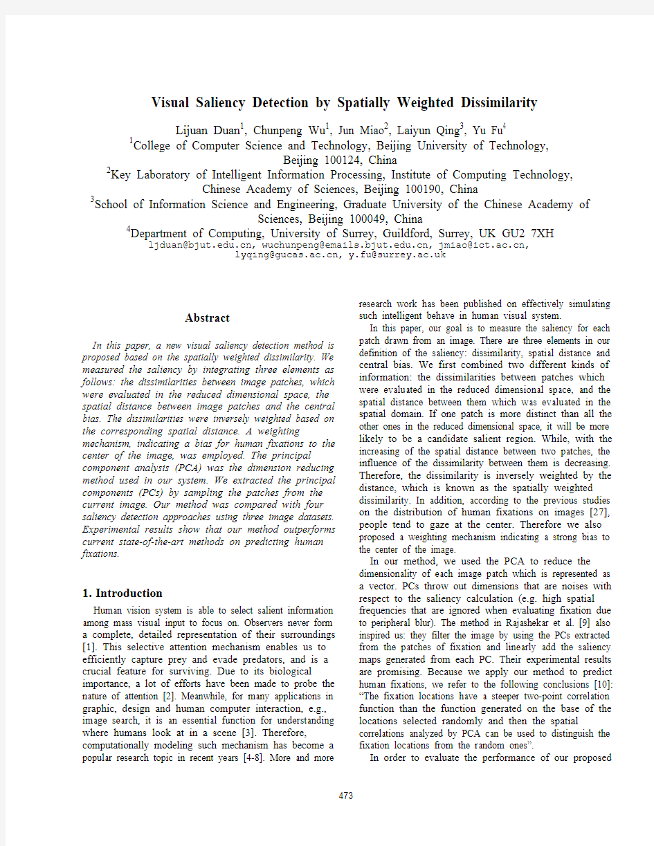
The proposed framework is shown in Fig. 1. There are three main steps in our method: representing image patches, reducing dimensionality and evaluating the spatially-weighted dissimilarity. Non-overlapping patches drawn from an image are represented as vectors of pixels. All patches are mapped into a reduced dimensional space. And then the saliency of each image patch is determined by aggregating the spatially-weighted dissimilarities between this patch and all the other ones in the image. The weighting mechanism indicating central bias is used in this step. Finally, the saliency map is normalized and resized to the scale of the original image, and then is smoothed with a Gaussian filter (3

σ=). In Fig. 1, for a better illustration, all patches are reduced to 3 dimensions which can be arbitrary in practice.

3.1.Image Patches Representation

Given an H W

×image I, non-overlapping patches with

the size of k k

×pixels are drawn from it. So the total number of patches is//

L H k W k

=?

????

????. A patch is

denoted as

i

p where1,2,...,

i L

=. Then, each patch is

represented as a column vector

i

f of pixel values. The length of the vector is2

3k, since the color space has three components. Finally, we get a sample matrix 1

[]

i L

=

2

A f f f f

"" where L is the total number of patches as stated above. In Section 4.2, we will comment on the effect if patches are allowed to overlap and the effect Figure 1: The framework of the proposed method. There are three main steps in our method: representing image patches, reducing dimensionality, and evaluating the spatially-weighted dissimilarity. The weight mechanism indicating the central bias

is used in the third step. In the figure, for a better illustration, all

patches are reduced to 3 dimensions which can be arbitrary in

practice.

if the grid divisions are allowed to arbitrarily locate.

3.2. Dimensionality Reduction

We aim to effectively describe patches in a relatively low dimensional space. As discussed in Section 1, we used an equivalent method to PCA to reduce data dimension. Each column in the matrix A subtracts the average along the columns. Then, we calculated the co-similarity matrix 2()/T L =G A A , therefore the size of the matrix G is L L ×. The eigenvalues and eigenvectors were calculated based on the matrix G and the biggest d eigenvalues were selected with their eigenvectors 12[,,,]T d =U X X X "

where i X is an eigenvector. The size of the matrix U is d L ×. As demonstrated in Fig. 1, a patch is mapped to a point in the reduced dimensional space and the positions of these points are determined by value of eigenvectors in matrix U . For example, the patch i p is represented by the corresponding column 1()T i i di x x =???U where i =1, 2,…, L . In Section 4.2, we will show the results of our method with and without the step of dimensionality reduction.

3.3. Evaluate Spatially Weighted Dissimilarity

There are two factors which were considered for evaluating the saliency: the dissimilarities between image patches in a reduced dimensional space, and their spatial distance. With the increasing of the spatial distance between two patches, the influence of the dissimilarity between them was decreasing. Therefore, the dissimilarities were inversely weighted by their corresponding spatial distances. Furthermore, the distance of each patch from the center of the image is involved in the evaluation of the saliency because of the central bias as stated in [3, 27]. With the increasing of the distance between a patch and the center, the saliency of the patch should be appropriately depreciated.

By integrating the elements of dissimilarity, spatial distance and central bias, the saliency of the patch i p is defined as follows

211()(){(,)(,)}L

j Saliency i i i j Dissimilarity i j ωω==??∑ (1)

where 1(,)i j ω is defined as

11

(,)1(,)

i j i j Dist p p ω=

+ (2)

where (,)i j Dist p p is the spatial distance between the two centers of patch i p and patch j p

in the image. The (,)Dissimilarity i j between the patch i p and patch j p in the reduced dimensional space is defined as

1

(,)||d

si sj s Dissimilarity i j x x ==?∑ (3)

In Equation (1), besides the weight 1ω representing the biological plausible characteristics which is similar to Mexican hat function, 2ωis the second weighting mechanism we proposed according to the average saliency map from human eye fixations indicating a bias to the center of image, which is shown at the bottom right of Fig. 4 in Judd et al. [3]. 2()i ω is defined as :

2()1()/i i DistToCenter p D ω=? (4)

where (

)i DistToCenter p is the spatial distance between two centers of patch i p and the patch at the center of the original image, and max {()}j j D DistToCenter p = is a normalization factor.

We will demonstrate in Section 4.2 that both spatially weighting mechanisms 1ω and 2ω play the significant role in saliency computing.

4. Experimental Validation

We applied our method on three public image datasets to evaluate its performance. Our method was compared with four different state-of-the-art saliency detection models based on a commonly-used validation approach. The same parameters of our method will be used across these datasets to illustrate its robustness.

Input Our method Human fixations

Figure 2: Results for a qualitative comparison between our

method and human fixations on the color image dataset 1. The first column show the input images, the second column is our

4.1. Parameters Selection

There are three parameters in our method: (1) the color space to which each patch is transformed (2) the dimension d to which each vector representing a patch is reduced (3) the size k of each patch. For color space, we choose YCbCr which is perceptually uniform and is a better approximation of the color processing in the human vision system as Gopalakrishnan et al. show in [20]. For each vector, the YCbCr channels are stacked after each other. We chose 11 as reduced dimension, because 11 is also the value that maximizes saliency predictions. The relationship between the dimensionality and the performance of our method will be shown in subsection 4.2. For the size k of each patch, we choose 14 because it is the smallest size that obtained maximal AUC. Also, the relationship between the size and the performance of our method will be shown in subsection 4.2.

4.2. Results on Color Image Dataset 1

The color image dataset which we used is introduced in Bruce et al. [6]. There are 120 images including indoor and outdoor scenes in the dataset, and 20 subjects’ fixations are recorded for each image （all the image sizes are 681× 511 pixels ）. To compare the saliency maps with the human fixations, we use the popular validation approach as Bruce et al. and Tatler et al. introduced in [6, 21]. The area under

the Receiver Operator Characteristics (ROC) curve, i.e., the area under the curve (AUC), was used to quantitatively evaluate the model performance.

Fig. 2 qualitatively shows the comparison between our saliency maps and the fixation density maps generated from the sum of all 2D Gaussians approximations of the drop-off of the density of the human fixations. We also compared our saliency maps with the other four state-of-the-art approaches [4, 6, 18, 19] in Fig. 3. The comparison results show that the most salient locations (the regions in the red circles in particular) on our saliency maps are more consistent with the human fixation density maps. For instance, in the fifth image, the car near the center is attended by human observers, but it is not detected to be salient by all the other saliency detection methods except ours. As demonstrated in Table 1, our method outperforms the other four methods on predicting human fixations. Furthermore, we compared the ROC curves in Fig. 4 which shows that our method achieves higher hit rates and lower false positive rates.

Table 1: Performances on the color image dataset 1

Attention Model AUC Improvement

Itti et al. [4] 0.7049 - Bruce et al. [6] 0.7613 0.0564 Hou et al. [18] 0.7923 0.0310 Harel et al. [19] 0.8021 0.0098 Our method 0.8333 0.0312

Input Itti Bruce Hou Harel Our method Human fixations

Figure 3: Results for a qualitative comparison between our method and the other four approaches on the color image dataset 1. The columns from the left to the right are: the input images, the saliency maps of Itti et al.’s method [4], Bruce et al.’s method [6], Hou et al.’s method [18], Harel et al.’s method [19], our method and the human fixation density maps. The most salient locations (the regions in the red circles in particular) on our saliency maps are more consistent with the human fixation density maps.

The results listed in Table 1 for those four compared methods are different from the results published in their corresponding papers [6, 18, 19]. This is because the sampling density which we used to obtain the thresholds is different with what they used. However, in our experiment, they were all evaluated on the same validation approach (we generated the ROC curves by using Harel et al. [19]’s code), so their relative performance should not be affected.

We compared the results generated by our method with and without doing dimensionality reduction. The comparison results are show in Fig 5. Based on these two curves, we investigated the relationship between the AUC area and the size of the image patches. In Fig. 5(a), although the trends of these two curves are nearly the same, we should notice that the method without dimensionality reduction always gets a smaller AUC for the same size of patches. Numerically, the average difference of AUC between these two methods is 0.02, which means that it is important to reduce the dimensionality according to the third column in Table 1. In Fig. 5(a), our proposed method (the red curve with circles) shows that the AUCs corresponding to the sizes of patches from 11 to 24 are above 0.83 and they are not significantly different. Among these sizes, we choose 14 as stated in subsection 4.1.

Then, in Fig. 5(b), we analyze the relationship between the AUC and the dimension d to which each vector representing an image patch is reduced, when the size k of image patch is 14. When the dimensionality d is bigger than 10, the AUC decreases as the dimensionality increases. That is to say, except the first few PCs, image patches is 14. In Fig. 5(b), when the dimensionality is bigger than 10, the AUC decreases as the dimensionality increases. That is to say, except the first few PCs, most of

the other ones rarely contribute to saliency detection . In fact, according to Hyv?rinen et al. [28], these PCs (except the first few ones) do not have meaningful spatial structure. In addition, in Fig. 5(b), the AUCs above 0.83 correspond to the dimensionality d from 6 to 17. To maximize saliency predictions, we choose d =11 in our method.

We also investigated the role of the two weighting

mechanisms 1ωand 2ω

as mentioned in Section 3.3. By setting 2ω to 1, the AUC decreases from 0.8333 to 0.7986, which is lower than the second largest AUC of 0.8021 by using Harel et al. [19]’s method. If we use the flat weights, i.e., 1ω and 2ω are set to 1, the AUC decreases from largely from 0.8333 to 0.7297. Therefore, both two spatially weighting mechanisms play the significant role in saliency computing.

(a)

(b)

Figure 5: (a) shows the comparison between our method with and without doing dimensionality reduction. Each curve illustrates the relationship between the AUC and the size k of patches. (b) shows the relationship between the AUC and the dimension d , when k is 14.

Figure 4: The ROC curves of our model and the other four approaches on the color image dataset 1.

As proposed in Section 3.1, non-overlapping patches are drawn from images in our method. When patches are half

overlapped, the AUC decreased from 0.8333 to 0.8276. This is because more similar patches produced near the current patch are given the higher weights by the item in Equation (1) and they decrease the dissimilarity between them and the current patch dominantly. However, the decreased AUC 0.8276 is still the highest result among other methods of the state of the art. In addition, adopting arbitrary location of grid divisions does not make a significant variation on the AUC results as shown in Table 2. For example, “Offset = 0.5” in Table 2 indicates that the grid divisions is moved with a 0.5 block size rightwards and downwards, the AUC has a little variation of -0.0006 and is still the highest result.

Table 2: Arbitrary location of grid divisions and AUC results

Offset (block size) AUC

0.1 0.8333 0.3 0.8322 0.5 0.8327 0.7 0.8300 0.9 0.8288 1.0 0.8293

4.3. Results on Color Image Dataset 2

We tested our method on another color image dataset introduced in Judd et al. [3]. The same parameters as stated in Section 4.1 were used. There are 1003 natural images containing different scenes and objects in this dataset, and the corresponding human fixations are also recorded. The size of the images in this dataset is not the same (the width

varies from 682 to 1024 pixels, and the height varies from 628 to 1024 pixels), which is different from the Bruce’s dataset used in Section 4.2. The AUC results and are shown in Table 3. Our method achieved the highest AUC results. The comparison between saliency maps is shown in Fig.6.

Table 3: Performances on the color image dataset 2

Attention Model AUC Bruce et al. [6] 0.7181 Hou et al. [18] 0.7625 Itti et al. [4] 0.7640 Harel et al. [19] 0.8172 Our method 0.8330

4.4. Results on Gray Image Dataset

The gray image dataset is DOVES which is introduced in van der Linde et al. [22]. The same parameters as stated in Section 4.1 are used. The DOVES dataset collects a set of visual eye movements from 29 human observers during viewing 101 natural calibrated images. We removed the first fixations of each eye movement trace superimposed on an image, because these fixations are forced fixations [22], they are not influenced by the saliency information on the current image. In Fig. 7, we compared our saliency maps with Itti et al.’s approach [4]. We used AUC to qualitatively evaluate the performance of our proposed method and the evaluating results are listed in Table 4.

Comparing to the AUC results on color images, the results on gray images do not decrease largely as shown in Table 4. However, the salient regions detected by Itti et al. [4]’s method and our method on gray images are not as consistent with human fixations as the regions detected by

Input Bruce Hou Itti Harel Our method Human Fixations

Figure 6: Results for a qualitative comparison between our method and the other four approaches on the color image dataset 2. The columns from the left to the right are: the input images, the saliency maps of Bruce et al.’s method [6], Hou et al.’s method [18], Itti et al.’s method [4], Harel et al.’s method [19], our method and the human fixation density maps.

these methods on color images. This might be because the images from the color image dataset contain semantic objects, but the images from the gray image dataset contain more raw signals. Meanwhile, Heidemann [23] stated that “for the same eigenvalue the corresponding PC from the color image has lower spatial frequency than the PC from the grey image, and features with lower spatial frequency are more preferable for many vision tasks (e.g., biological vision task) for they are more robust against translation or image distortion”.

Table 4: Performances on the gray image dataset

Attention model Itti et al. [4] Our method AUC 0.7101

0.8352

5.Discussions

The saliency maps produced by our method are a little spread out, i.e., large regions of the image appear to all be quite saliency. On the contrary, Achanta et al. [8]’s method generated sharper and uniformly highlighted salient regions. Using the above method of ROC curve, we found the AUC of [8] was smaller than the results by using Harel et al. [19] and our method. As pointed out by [8], “the true usefulness of a saliency map is determined by the application”. Our saliency maps contain information from several elements of biological plausible characteristics. We can get different salient regions by setting different thresholds for different visual tasks. For example, by setting a higher threshold, the saliency map may produce sparse salient regions approximating human fixations; by setting a lower threshold, the diffuse saliency map may produce the “coarse segmentation” effect that means salient regions contain salient objects. Based on it, the skeleton features can be extracted and used for fine segmentation. As shown

in Achanta et al. [8] and Yu et al. [26], their work indicated the possible application of the proposed method for saliency-guided segmentation.

6.Conclusions and Future Work

In this paper, we have presented a visual saliency detection method. To measure the saliency, we actually combine spatially weighted dissimilarity with a weighting mechanism indicating central bias for human fixations. In Section 4.2, we demonstrate the significant role of the above two weighing mechanisms. We extract PCs by sampling the patches from current image, because we suppose that PCA over patches within each image emphasize the variability within the image, which is what will drive fixation. Experimental results on three public image datasets show that our method outperforms some state-of-the-art saliency detection approaches on predicting human fixations. The saliency maps produced by our method are spread out; however, we can get different salient regions by setting different thresholds for different visual tasks.

One of the limitations of the PCA is that it only captures the structure of data in which the linear pairwise correlations are the most important form of statistical dependence [24]. Therefore we are considering how to extend our analysis to include the non-linear dependencies

in the data. Also, the size of the image patches was predefined, and the image was not represented in a multi-scale way. Therefore, the performance of our method may be degraded on the multi-scales visual attention regions. In future, we will extend our work to find a mechanism which can select suitable scales for a particular location. In addition, in our PCA-based method, the 2D image patches must be transformed into 1D vectors, so the resulting vectors lead to a high dimensional space. To spend less time on determining the corresponding eigenvectors and evaluate the covariance matrix more accurately, we will try to use the two-dimensional PCA introduced in Yang et al. [25], which does not transform the image matrix into a vector.

Acknowledgement. The authors would like to thank the technical assistance from the graduate student Chen Chi and the helpful discussion with Dr. Zhen Yang and Dr. Yuzhi Chen. This research is partially sponsored by National Basic Research Program of China (No.2009CB320902), Hi-Tech Research and Development Program of China (No.2006AA01Z122), Beijing Natural Science Foundation(Nos.4072023 and 4102013), Natural Science Foundation of China (Nos.60702031, 60970087, 61070116, 61070149 and 60802067) and President Fund of Graduate University of Chinese Academy of Sciences (No.085102HN00).

Input Itti Our method Human Figure 7: Results for a qualitative comparison between our method and Itti et al.’s approach [4] on the gray image dataset. The first column is input images, the second columns is the saliency maps of Itti et al.’s method, the third column is the saliency maps of our method, and the fourth column is the human fixation density maps.

References

[1]R. Rensink, K. O’Regan, J. Clark. To see or not to see: The

need for attention to perceive changes in scenes. In:

Psychological Sciences, 1997.

[2]J. K. Tsotsos, L. Itti and G. Rees. A brief and selective

history of attention. In: Neurobiology of Attention, Editors

Itti, Rees & Tsotsos, Elsevier Press, 2005.

[3]T. Judd, K. Ehinger, F. Durand and A. Torralba. Learning to

predict where humans look. In: ICCV, 2009.

[4]L. Itti, C. Koch and E. Niebur. A model of saliency-based

visual attention for rapid scene analysis. In: PAMI, 1998. [5]T. Kadir and M. Brady. Saliency, scale and image

description. In: IJCV, 2001.

[6]N. D. B. Bruce and J. K. Tsotsos. Saliency based on

information maximization. In: NIPS, 2005.

[7] D. Gao and N. Vasconcelos. Bottom-up saliency is a

discriminant process. In: ICCV, 2007.

[8]R. Achanta, S. Hemami, F. Estrada and S. Susstrunk.

Frequency-tuned salient region detection. In: CVPR, 2009. [9]U. Rajashekar, L. K. Cormack and A. C. Bovik. Image

features that draw fixations. ICIP, 2003.

[10]P. Reinagel and A. M. Zador. Natural scene statistics at the

centre of gaze. Network: Computation in Neural Systems,

1999.

[11]A. M. Treisman and G. Gelade. A feature-integration theory

of attention. Cognitive Psychology, 1980.

[12]T. Liu, J. Sun, N. N. Zheng, X. Tang and H. Y. Shum.

Learning to detect a salient object. CVPR, 2007.

[13]V. Gopalakrishnan, Y. Hu and D. Rajan. Salient region

detection by modeling distributions of color and orientation.

IEEE Transactions on Multimedia, 2009.

[14]W. Kienzle, M. O. Franz, B. Scholkopf and F. A. Wichmann.

Center-surround patterns emerge as optimal predictors for

human saccade targets. Journal of Vision, 2009.

[15]X. Hou and L. Zhang. Saliency detection: A spectral residual

approach. CVPR, 2007.

[16]C. Guo, Q. Ma and L. Zhang. Spatio-temporal saliency

detection using phase spectrum of quaternion fourier transform. CVPR, 2008.

[17]J. Gluckman. Higher order whitening of natural images.

CVPR, 2005.

[18]X. Hou and L. Zhang. Dynamic visual attention: Searching

for coding length increments. NIPS, 2008.

[19]J. Harel, C. Koch and P. Perona. Graph-based visual

saliency. NIPS, 2006.

[20]V. Gopalakrishnan, Y. Hu and D. Rajan. Random walks on

graphs to model saliency in images. CVPR, 2009.

[21]B. W. Tatler, R. J. Baddeley, I. D. Gilchrist. Visual correlates

of fixation selection: effects of scale and time. Vision

Research, 2005.

[22]I. van der Linde, U. Rajashekar, A.C. Bovik, and L.K.

Cormack, DOVES: A database of visual eye movements.

Spatial Vision, 2009.

[23]G. Heidemann. The principal components of natural images

revisited. PAMI, 2006.

[24]B. A. Olshausen and D. J. Field. Emergence of simple-cell

receptive field properties by learning a sparse code for

natural images. Nature, 1996.

[25]J. Yang, D. Zhang, A. F. Frangi and J. Y. Yang.

Two-dimensional PCA: A New Approach to

Appearance-Based Face Representation and Recognition.

PAMI, 2004.

[26]H. Yu, J. Li, Y. Tian and T. Huang. Automatic interesting

object extraction from images using complementary saliency maps. ACM International Conference on Multimedia, 2010.

[27]B. W. Tatler. The central fixation bias in scene viewing:

Selecting an optimal viewing position independently of motor biases and image feature distributions. Journal of Vision, 2007.

[28]A. Hyv?rinen, J. Hur r i, and P. O. Hoyer. Natur al Image

Statistics: A Probabilistic Approach to Early Computational Vision, Springer: London, 2009.