3+1 formulation of non-ideal hydrodynamics
甜菜碱型两性离子聚合物P(AM-DMAPAAS)的盐溶液性质

甜菜碱型两性离子聚合物P(AM-DMAPAAS)的盐溶液性质丁伟;毛程;韦兆水;李明;于涛;曲广淼【期刊名称】《应用化学》【年(卷),期】2011(28)5【摘要】将丙烯酰胺丙基二甲基胺(DMAPAA)和1,3-丙基磺内酯,在55℃下反应20 h,合成了3-(丙烯酰胺丙基二甲胺基)丙磺酸盐(DMAPAAS),将其在盐溶液中与丙烯酰胺(AM)单体进行自由基共聚合反应,获得净电荷为零的磺基甜菜碱型两性离子共聚物P(AM-DMAPAAS);对该两性离子共聚物进行了表征和溶解性评价.研究结果表明,共聚物在NaCl溶液中的粘度比在纯水中的大,在Mg(2+)和Ca(2+)盐溶液中的粘度更大,且随着溶液浓度的增大而增大,表现出明显的反聚电解质溶液性质.升高相同温度,两性离子共聚物的粘度保留率是普通聚丙烯酰胺的1.4倍.%A zwitterionic monomer of 3-( N, N-dimethylamino-N-sulfopropane propyl acrylamide ) (DMAPAAS) was prepared by the ring opening reaction of 1,3-cyclopropanesultone with N,N-dimethylamino propyl acrylamide( DMAPAA) at 55 ℃ for 20 h. Zwitterionic copolymers P ( AM-DMAPAAS) containing sulfobetaine groups were synthesized by copolymerization of AM and DMAPAAS in aqueous solution. The copolymers were characterized and the solubility of copolymers P ( AM-DMAPAAS) was evaluated. The viscosity of the copolymers was determined. The results show that the viscosity of the copolymers in brine solution is greater than that in deionized water, and the viscosity in Mg2+ and Ca2+ salt solution is increased as the salt concentration is increased. The copolymers exhibita typical antipolyelectrolyte behavior. Under the situation where the same temperature is increased, the viscosity retention of the zwitterionic copolymer is 1. 4 times of that of PAM.【总页数】5页(P555-559)【作者】丁伟;毛程;韦兆水;李明;于涛;曲广淼【作者单位】东北石油大学,化学化工学院,大庆,163318;东北石油大学,化学化工学院,大庆,163318;东北石油大学,化学化工学院,大庆,163318;东北石油大学,化学化工学院,大庆,163318;东北石油大学,化学化工学院,大庆,163318;东北石油大学,化学化工学院,大庆,163318【正文语种】中文【中图分类】O631【相关文献】1.磺基甜菜碱型两性离子聚合物的盐溶液性质 [J], 毛程;丁伟;于涛;曲广淼2.磺基甜菜碱型两性离子聚合物的合成 [J], 丁伟;毛程;于涛;刘宏彬;曲广淼3.甜菜碱型两性离子聚合物的水解及其对抗菌性能影响的研究 [J], 刘东立;陈昌林;郎美东4.羧基甜菜碱型两性离子聚氨酯水凝胶的制备及水下抗原油黏附性能 [J], 王阿强;朱玉长;靳健5.含磺酸甜菜碱两性离子共聚物P(AM-co-VPPS)的合成及盐溶液性质 [J], 桂张良;安全福;曾俊焘;徐红;钱锦文因版权原因,仅展示原文概要,查看原文内容请购买。
锂离子电池非水电解质中Li +迁移特性
收稿:2006年12月,收修改稿:2007年5月 3通讯联系人 e 2mail :hexm @锂离子电池非水电解质中的Li +迁移特性赵吉诗 王 莉 何向明3 姜长印 万春荣(清华大学核能与新能源技术研究院 北京102201)摘 要 电解质是锂离子电池的重要组成部分之一,其中Li +的迁移特性对电池性能具有显著影响。
本文综述了用于锂离子电池的凝胶、聚合物和非水液态电解质中Li +迁移特性的研究进展,分析了影响Li +迁移的主要因素,并提出了进一步的研究重点和新的研究方法。
关键词 锂离子电池 非水电解质 电导率 Li +迁移数中图分类号:O646;T M911 文献标识码:A 文章编号:10052281X (2007)1021467208Transport Properties of Lithium 2Ion of E lectrolyte Usedin Lithium 2Ion B atteriesZhao Jishi Wang Li He Xiangming3 Jiang Changyin Wan Chunrong(Institute of Nuclear &New Energy T echnology ,Tsinghua University ,Beijing 102201,China )Abstract The ability to conduct ions is the basic function of non 2aqueous electrolytes used in the lithium 2ion batteries.It determines how fast the energy stored in electrodes can be delivered.Recent advances of the transport properties of the lithium ion in the non 2aqueous electrolyte including the gel ,polymer and liquid systems are reviewed.The factors in fluencing the trans fer of the lithium ion and the prospects of the research are als o discussed.K ey w ords lithium 2ion batteries ;non 2aqueous electrolyte ;conductivity ;lithium 2ion transport number1 引言锂离子电池已经在便携式电子设备中得到了广泛的应用,随着信息时代的到来,其应用范围正在迅速扩展。
非线性动态方法评估重合钢筋建筑的地震抗性说明书
7th International Conference on Mechatronics, Control and Materials (ICMCM 2016)Assessment of seismic resistance of the reinforced concrete buildingby nonlinear dynamic methodOleg Vartanovich Mkrtychev1, Marina Sergeevna Busalova2*1Head of the Research laboratory “Safety and Seismic Resistance of Structures” Professor of theDepartment “Strength of Materials”Moscow State University of Civil Engineering (National Research University) 26, YaroslavskoeShosse, Moscow, Russia2Engineer of the Research laboratory “Safety and Seismic Resistance of Structures” Moscow State University of Civil Engineering (National Research University) 26, Yaroslavskoe Shosse, Moscow,Russia**************************Keywords:direct dynamic method, non-linearity, seismic impact, reinforced concrete structures, near-collapse criterion.Abstract.The article studies the reaction of the 5-storey reinforced concrete building of the cross-sectional wall structural scheme to the seismic impact. Bearing structures of the building were simulated by the three-dimensional finite elements, connecting concrete and reinforcement, in the software application LS-DYNA. The calculation was carried out by the direct dynamic method using the directly integrated equation of motion according to the explicit scheme. Using this method for calculation allows to make calculations in the temporary area and also to take into account the nonlinearities in the analytic model. In particular, the physical non-linearity is taken into account by means of the non-linear diagram of the concrete deformation. To create an adequate analytic-dynamic model the authors of the article developed the method allowing to take into account the actual reinforcement of the structure. The research conducted allows to estimate the reaction of the 5-storey reinforced concrete building to the set seismic impact.IntroductionThe base of the edition of SP 14.13330.2014 SNiP II-7-81* “Construction in Seismic Regions” [1] acting since 2015 takes the requirements of the two-level calculation of the seismic impact. The earthquake analysis corresponding to the level of the maximal design earthquake shall be performed according to the near-collapse criterion. It means that the calculation methods shall directly take into account the non-linear character of the structural deformation (physical, geometrical, structural non-linearities). However, now in Russia the corresponding method and verified dynamic model allowing to make calculations at the level of maximal design earthquake are not available. The authors of the article developed the method allowing to take into account the non-linear properties of concrete when making calculations of seismic impact, and also to include the elements of the connection of concrete and reinforcement into the analytical model taking into account the actual reinforcement of the structure.Setting of problemConcrete is a complicated composite material that consists mostly of the filling and the grouting, and at the different impacts its reaction can vary from brittle fracture at tensioning to yield behavior at compression. Non-linear diagram of concrete deformation taking into account the physical non-linearity is shown in the Figure 1 [2].Figure 1. Non-linear diagram of concrete deformationTo solve the problem it is necessary to have a corresponding material model. The Figure 2 shows the most complete models describing adequately the work of concrete at deformation (CSCM – Continuous Surface Cap Model) [3].Figure 2. Mathematical model of concrete (CSCM – Continuous Surface Cap Model) Concrete yield surface is described by the invariants of the stress tensor that in turn are determined from the formula (1)-(3).13J P=(1)212ij ijJ S S′=(2)313ij jk kiJ S S S′=(3)where1J is the first invariant of the stress tensor, 2J′ is the second invariant of the stress tensor, 3J′is the third invariant of the stress tensor,ijS is stress tensor, P is pressure.To study the actual reaction of the structure to the seismic impact it will not be sufficient to take into account the nonlinear properties of the concrete only. To show the real picture of thedeformation it is necessary to include the actual reinforcement into the analytic dynamic model, that is, to simulate the reinforcement cage of the building under analysis in the structural design [4].The Figure 3 shows the structural design of the five-storey reinforced concrete building of the cross-sectional wall structural scheme. All bearing structures are simulated by the three dimensional elements for concrete and bar elements for reinforcement [5].Figure 3. Structural design The Figure 4 shows the reinforcement cages of the building.Figure 4. Reinforcement cageCalculation resultsCalculation was made by the software application LS-DYNA by the direct dynamic method [6]. Equations of motion (4) were integrated directly according to the explicit scheme (5):a ++=Mu Cu Ku f (4)where u is nodal displacement vector, =uv is nodal velocity vector, =u a is nodal acceleration vector, M is mass matrix, C is damping matrix, K is rigidity matrix, af is vector of applied loads. /22t t t t t t t t t t +∆+∆+∆∆+∆=+u u v (5)This method allows to take into account the geometrical, physical and structural nonlinearities andalso to make calculations in the temporary area (dynamics in time).Three-component diagram was used as a design seismic impact corresponding to the intensity 9 earthquake (Figure 5). a)b)c)Figure 5. Three-component accelerograma)component X, b) component Y, c) component ZIsofields of the plastic deformations after the earthquake (t = 30 s) are shown in the Figure 6. Figure 6. Isofields of the plastic deformations after the earthquake at the moment of time t = 30 s The character of the plastic deformations corresponds completely to the character of cracks distribution. The Figure 6 shows that the bearing structures of the building of this structural scheme were damaged seriously but the building did not collapse, that means the conditions of the special limit state (near-collapse criterion) are satisfied. As a result of the conducted research, the seismic resistance of the building according to the near-collapse criterion was determined as intensity 9.ConclusionsThe analysis of the data obtained as a result of the research allows to conclude that for the adequate estimation of the reaction of the structure to the seismic impact it is necessary to make calculations in the nonlinear dynamic arrangement taking into account the nonlinear diagrams of concrete deformation and also to add the actual reinforcement into the structural design. The use of the offered method of the buildings earthquake calculations at the design stage will allow to estimate adequately the level of seismic resistance of the building structures.AcknowledgementsThis study was performed with the support of RF Ministry of Education and Science, grant No.7.2122.2014/K.References[1].SP 14.13330.2014 SNIP II-7-81. Stroitel'stvo v seysmicheskikh rayonakh[SP 14.13330.2014SNIP II-7-81. Construction in Seismic Areas]. (2014). Moscow: Analitik.[2].SP 63.13330.2012 SNIP 52-01-2003. Betonnye i zhelezobetonnye konstruktsii. Osnovnyepolozheniya[SP 63.13330.2012 SNIP 52-01-2003. Concrete and Reinforced Concrete Structures. Summary]. (2012). Moscow: Analitik.[3].Murray, Y.D. (2007). Users Manual for LS-DYNA Concrete Material Model 159. Report No.FHWA-HRT-05-062. U.S. Department of Transportation: Federal Highway Administration. [4].Murray, Y.D. (2007). Evaluation of LS-DYNA Concrete Material Model 159. Publication No.FHWA-HRT-05-063. U.S. Department of Transportation: Federal Highway Administration. [5].LS-DYNA. (n.d.). Keyword User’s Manual(Vol. 1, 2). Livermore Software TechnologyCorporation (LSTC).[6].Andreev, V.I., Mkrtychev, O.V., & Dzinchvelashvili, G.A. (2014). Calculation of Long SpanStructures to Seismic and Accidental Impacts in Nonlinear Dynamic Formulation. Applied Mechanics and Materials, 670-671, 764-768。
MaterialModeling-3

The Influence of Permanent Volumetric Deformationon the Reduction of the Load Bearing Capabilityof Plastic ComponentsP.A. Du Bois*, S. Kolling**, M. Feucht***, A. Haufe*****Consultant, Freiligrathstr. 6, 63071 Offenburg, Germany**Gießen University of Applied Sciences, 35390 Gießen, Germanystefan.kolling@mmew.fh-giessen.de***Daimler AG, EP/SPB, 71059 Sindelfingen, Germanymarkus.feucht@****DYNAmore GmbH, Industriestrasse 2, 70565 Stuttgart, Germanyandre.haufe@dynamore.deAbstractDuring the past years polymer materials have gained enormous importance in the automotive industry. Especially their application for interior parts to help in passenger safety load cases and their use for bumper fascias in pedes-trian safety load cases have driven the demand for much more realistic finite element simulations. For such applica-tions the material model 187 (i.e. MAT_SAMP-1) in LS-DYNA® has been developed.In the present paper the authors show how the parameters for the rather general model may be adjusted to allow for the simulation of crazing effects during plastic loading. Crazing is usually understood as inelastic deformation that exhibits permanent volumetric deformations. Hence a material model that is intended to be applied for polymer components that show crazing effects during the experimental study, should be capable to produce the correct volu-metric strains during the respective finite element simulation. The paper discusses the real world effect of crazing, the ideas to capture these effect in a numerical model and exemplifies the theoretical ideas with a real world struc-tural component finite element model.IntroductionCrazing is generally understood as the formation of micro cracks as sketched in Figure 1 (the mi-crograph is taken from [16]). As a consequence thereof, the change of color to white is visibly detectable since the crack-lengths become the magnitude of the wavelength of light. From a me-chanical point of view, crazing leads to plastic (i.e. permanent) deformation accompanied by an increase of volume. Since surface cracks occur preferably under biaxial loading, crazing leads to low yield stress values in uniaxial/biaxial tension that can also be detected experimentally. It also seems to occur under high values of hydrostatic tension. In the present paper, the authors like to show how these effects can be captured in a phenomenological way by using non-isochoric plas-ticity and ductile damage.Figure 1: Formation of crazingNumerical TreatmentIn the present study, we used the SAMP-model suggested in [11]. This model combines non-isochoric plasticity and ductile damage. The advantage of this model is that all required input data may be provided in a tabulated way. Thus no parameter identification is necessary which represents an important factor in daily practice. See e.g. [13] for an overview of ductile damage models in LS-DYNA ® in comparison with the tabulated damage model in SAMP. In what fol-lows we give a short overview of the SAMP-model and the corresponding damage formulation.Yield Surface and Plastic Potential in SAMPThe basic idea of SAMP is illustrated in Figure 2. Starting point is the definition of a pressure depending, quadratic yield surface()0,,22102≤−−−=p A p A A p f vm p vm σεσ .(1)This yield surface is defined by three independent stress states in the invariant plane following from tensile, compression, shear or biaxial stress for a fixed plastic strain during hardening. The hardening curve may be given in a tabulated way as it is well known from MAT_PIECE-WISE_LINEAR_PLASTICTY. The strain rate dependency is defined by tabulated tensile curves, i.e. the strain rate behaviour is assumed to be identically for all stress states. If less than three stress states are provided, the SAMP yield surface degenerates to a Drucker-Prager model (see [4], 2 curves are used) and a von Mises model (1 curve) respectively. Providing usually ten-sile, compression and shear data, the SAMP-coefficients are computed from the hardening curves internally bysFigure 2: Yield surface in SAMP (Semi-Analytical Model for Polymers)In order to simulate crazing, the increase of volume during plastic flow is taken into account by defining the plastic potential22p g vm ασ+=. (2)The parameter α is determined internally if a plastic Poisson ratio νp (lateral strain rate over lon-gitudinal strain rate) is provided by the user: i.e. either by a constant value or in a tabulated way as a function of longitudinal strain. In this context, it is also possible to define different behav-iour under tension and compression. In the latter case, thermoplastics do not show volume in-crease so that it is recommended to define νp =0.5=const under pressure.Damage Models in SAMPThe model uses the notion of the effective cross section, which is the true cross section of the material minus the cracks that have developed. We define the effective stress as the force divided by the effective cross sectionA F =σ, dd A F A F eff eff −=−==11σσ (3) which allows defining an effective yield stress of dyeff y −=1,σσ. The damaged yield function inSAMP is given by()()02122211A d p A d p A vm −−−−−=Φσ (4)2220123399c t c t s ss c t c t A A A σσσσσσσ⎛⎞⎛⎞−−===⎜⎟⎜⎟⎝⎠⎝⎠By application of the principle of strain equivalence, stating that if the undamaged modulus is used, the effective stress corresponds to the same elastic strain as the true stress using the dam-aged modulus, one can write ()d E E E ede eff −===1,εσεσ. Note that the plastic strains are therefore the same: deffp E E σεσεε−=−=. No damage will occur under pure elastic deforma-tion with this model. Among others, the damage model represents a good approximation to fit the unloading behavior of plastics [6]. A similar model is given by Lemaitre, where the damaged yield function is given by()()eff p eff y vm d ,2,221εσσ−−=Φ ,(5)which leads to the same formulation as SAMP if we set 021==A A and 2,0eff y A σ=. For a com-parison of the chosen model with the formulation by Gurson we may rewrite ()0123cosh 22*1,2*12,2=−−⎟⎟⎠⎞⎜⎜⎝⎛−+=Φf q p q f q eff y eff y vm σσσ . (6)With ()221cosh x x +≈ we obtain a Taylor-approximation of Gurson's yield surface by()2,2222*12*1149eff y vm f q p q f q σσ−−+≈Φ . (7)Figure 3: Evolution of the yield surface in function of damage in invariant planef*=0.00 f*=0.05 f*=0.10 f*=0.15 f*=0.20Comparison with Equation (4) yields the SAMP-parameters to be *1f q d =, 2,0eff y A σ=, 01=Aand t dq A cons 49222≠−=. Note that the last term is non-constant, i.e. the shape of the yield sur-face changes with increasing damage, see Figure 3. A comparison of the damage model in SAMP with Gurson's formulation, where Gurson's evolution law is approximated in SAMP by an equivalent tabulated input consisting of damage in function of plastic strain can be found in the study [15].ApplicationAs an industrial application we show a validation procedure for a structural part taken from a bumper that is made from PP T10. The experimental setup consists of a compression test on the structural component (Figure 4). In the picture in the middle, the formation of crazing can be ob-served very nicely. The intent of the present study is, on the one hand, to demonstrate the impor-tance to consider the different behavior of thermoplastics under tension and compression. And, on the other hand, to represent crazing of the thermoplastic as it occurs in real-world-experiments.Figure 4: Component testIn the first step, strain rate dependent tensile tests are performed and a material card is fitted solely from this tensile tests. We start our component validation with a standard material model in LS-DYNA: MAT_PIECEWISE_LINEAR_PLASTICTY (Mat No. 24). In order to investigate the mesh dependency we provide two meshes: A fine mesh (1mm element size) and a coarse mesh (6mm element size), see Figure 5.Figure 5: Coarse mesh (6mm element size) and fine mesh (1mm element size)displacementf o r c eFigure 6: Force-displacement in comparison with the experiment: Mat No. 24 vs. SAMPThe problem of material cards which are fitted entirely under tension consists of the fact that there is no guarantee that it also works for multi-axial loading. In the present component test we have bending and, nearly exclusive, compression. The force-displacement-diagram in Figure 6 shows a typical behavior for thermoplastics: Material cards that are fitted for uniaxial tension yield a too soft response under bending and compression. Mat. No. 24 (dashed line) is therefore not capable to fit the experiment (dotted line) and, thus, different yield curves under compression and tension are necessary! This has been done in SAMP where a Drucker-Prager-model has been generated by scaling the tensile date by a factor 1.3 in the compressive region. This model is al-ready in a very good agreement with the experimental data, though the range in the diagram where cracks occur are still too stiff. This is a topic of further investigation in near future.displacementf o r c eFigure 7: Influence of meshinga) Mat. No. 24b) SAMPFigure 8: Crazing: Mat No. 24 vs. SAMP (coarse mesh)Figure 7 shows the influence of using a coarse mesh and a fine mesh. As expected, the coarse mesh yields to a slightly stiffer response. This has also to be taking into account in full-car-simulations where the average element size is rather 5mm than 1mm. Further study has shown that mesh convergence will be reached for approximately 2mm element characteristic length.At last, crazing of the component is approached by using the following SAMP-features:− plastic Poisson’s ratio decreases with increasing plastic strain (further input curve) − plastic incompressibility under compression − reduced biaxial strength (further input curve)− damage evolution is considered (further input curve)Figures 8 and 9 show the results of the simulation in comparison to Mat No. 24. As can be seen, the deformation behavior (see Figure 4) cannot be reproduced by using Mat No. 24. We obtain a totally different (and wrong) buckling mode. The simulation using SAMP together with the fea-tures described above yields to a quite more realistic deformation behavior. Moreover, the region of plastic volumetric strain (which is zero in Mat No. 24) represents a one-to-one relation to the region of crazing in the structural part. With other words, the effect of crazing cannot be simu-lated by any isochoric elasto-plastic material law! The craze deformation can be further im-proved by using the fine mesh (see Figure 9b).a) Mat. No. 24 b) SAMPFigure 9: Crazing: Mat No. 24 vs. SAMP (fine mesh)Summary and OutlookMatching a measured force-displacement curve in a simulation should be phase 2 of the valida-tion process. The numerical model will have a very limited range of validity unless the deforma-tion (and failure) mode in the simulation correspond to what was observed. It seems useful to consider a coupling between damage and volumetric plastic strain in the simulation of thermo-plastics. A combination of volumetric plastic strain, damage and reduced biaxial strength al-lowed to simulate the craze deformation in a rather complex structural part. The influence of crack formation and crack propagation is topic of further investigation in the near future.References[1]LS-DYNA®, Theory Manual / Keyword User’s Manual, Livermore Software Technology Corporation.[2]P.A. Du Bois: Crashworthiness Engineering Course Notes, Livermore Software Technology Corporation,2004.[3]S. Kolling, A. Haufe: A constitutive model for thermoplastic materials subjected to high strain rates, Proceed-ings in Applied Mathematics and Mechanics • PAMM 5: 303-304.[4] D.C. Drucker, W. Prager: Soil mechanics and plastic analysis or limit design. Quaterly of Applied Mathemat-ics, 10:157-165, 1952.[5]V.A. Kolupaev, S. Kolling, A. Bolchoun, M. Moneke: A limit surface formulation for plastically compressi-ble polymers. Mechanics of Composite Materials, 43(3):245--258, 2007.[6]P. A. Du Bois, S. Kolling, M. Koesters, T. Frank: Material behavior of polymers under impact loading. Inter-national Journal of Impact Engineering 32 (2006) 725-740.[7]J.C. Simo, T.J.-R. Hughes: Elastoplasticity and viscoplasticity – computational aspects. Springer Series inApplied Mathematics, Springer, Berlin, 1989.[8]T.J.-R. Hughes: Efficient and simple algorithms for the integration of general classes of inelastic constitutiveequations including damage and rate effects. In T.J.-R. Hughes, T. Belytschko: nonlinear finite element analysis course notes, 2003.[9]J. Lemaitre, J.-L. Chaboche: Mécanique des matériaux solides, Dunod, 1988.[10]W.W. Feng, W.H. Yang: general and specific quadratic yield functions, composites technology review.[11]S. Kolling, A. Haufe, M. Feucht, P.A. Du Bois: A semianalytical model for the simulation of polymers. 4thLS-DYNA Forum, Germany 2005, Conference Proceedings, ISBN 3-9809901-1-7, pp. A-II-27/52.[12]M. Vogler, R. Rolfes, S. Kolling: Orthotropic plasticity with application to fibre-reinforced thermoplastics.Proceedings of the 6th LS-DYNA Forum Meeting, Frankenthal, Germany, D-II:55-74, 2007.[13]P.A. Du Bois, M. Feucht, S. Kolling, A. Haufe: An overview of ductile damage models in LS-DYNA. Pro-ceedings of the 6th LS-DYNA Forum Meeting, Frankenthal, Germany, Keynote-Lectures I, pp 1-17, 2007. [14]M. Vogler, S. Kolling and A. Haufe: A constitutive model for plastics with piecewise linear yield surface anddamage. Proceedings of the 6th LS-DYNA Forum Meeting, Frankenthal, Germany, B-II:13-30, 2007. [15]P.A. Du Bois, S. Kolling, M. Feucht, A. Haufe: A comparative review of damage and failure models and atabulated generalization. Proceedings of the 6th European LS-DYNA Users Conference, Gothenburg, Swe-den, pages 75-86, 2007.[16]J. Rottler, M.O. Robbins: Growth, microstructure, and failure of crazes in glassy polymers, Phys Rev E, 68,011801, 2003.。
LS-DYNA 理论及功能(简介)
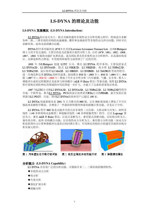
LS-DYNA 理论及功能LS-DYNA 的理论及功能LS-DYNA 发展概况 (LS-DYNA Introduction)LS-DYNA是以显式为主、隐式为辅的通用非线性动力分析有限元程序,特别适合求解 各种二维、三维非线性结构的高速碰撞、爆炸和金属成形等非线性动力冲击问题,同时可以 求解传热、流体及流固耦合问题。
DYNA 程序系列最初是 1976 年在美国 Lawrence Livermore National Lab. 由 J.O.Hallquist 博士主持开发完成的,主要目的是为武器设计提供分析工具,后经 1979、1981、1982、1986、 1987、1988 年版的功能扩充和改进,成为国际著名的非线性动力分析软件,在武器结构设 计、内弹道和终点弹道、军用材料研制等方面得到了广泛的应用。
1988 年 J.O.Hallquist 创建 LSTC 公司,推出 LS-DYNA 程序系列,主要包括显式 LS-DYNA2D、LS-DYNA3D、隐式 LS-NIKE2D、LS-NIKE3D、热分析 LS-TOPAZ2D、 LS-TOPAZ3D、前后处理 LS-MAZE、LS-ORION、LS-INGRID、LS-TAURUS 等商用程序, 进一步规范和完善 DYNA 的研究成果,陆续推出 930 版(1993 年)、936 版(1994 年)、940 版(1997 年),950 版(1998 年)增加了汽车安全性分析(汽车碰撞、气囊、安全带、假人)、 薄板冲压成形过程模拟以及流体与固体耦合(ALE 和 Euler 算法)等新功能,使得 LS-DYNA 程序系统在国防和民用领域的应用范围进一步扩大,并建立了完备的质量保证体系。
1997 年LSTC公司将LS-DYNA2D、LS-DYNA3D、LS-TOPAZ2D、LS-TOPAZ3D等程序 合成一个软件包,称为LS-DYNA,PC版的前后处理采用ETA公司的FEMB,新开发的后处 理器为LS-POST。
非牛顿流体电动力学外文文献翻译、中英文翻译、外文翻译
论文翻译原文:Electrokinetics of non-Newtonian fluids: A reviewABSTRACTThis work presents a comprehensive review of electrokinetics pertaining to non-Newtonian fluids. The topic covers a broad range of non-Newtonian effects in electrokinetics, including electroosmosis of non-Newtonian fluids, electrophoresis of particles in non-Newtonian fluids, streaming potential effect of non-Newtonian fluids and other related non-Newtonian effects in electrokinetics. Generally, the coupling between non-Newtonian hydrodynamics and electrostatics not only complicates the electrokinetics but also causes the fluid/particle velocity to be nonlinearly dependent on the strength of external electric field and/or the zeta potential. Shear-thinning nature of liquids tends to enhance electrokinetic phenomena, while shear-thickening nature of liquids leads to the reduction of electrokinetic effects. In addition, directions for the future studies are suggested and several theoretical issues in non-Newtonian electrokinetics are highlighted.1. IntroductionThe recently growing interests in electrokinetic phenomena are triggered by their diverse applications in microfluidic devices which could have the potential to revolutionize conventionalways of chemical analysis,medical diagnostics, material synthesis, drug screening and delivery aswell as environmental detection andmonitoring. The prevalent use of electrokinetic techniques in microfluidic devices is ascribed to their several distinctive advantages: (i) the devices are energized by electricitywhich is widely available and ease of control; (ii) the devices involve no moving parts and thus less mechanical failures; (iii) the induced velocity of liquid or particle is independent of geometric dimensions of devices; (iv) the devices can be readily integrated with other electronic controlling units to achieve fully-automated operation. In addition to its useful applications in microfluidics, electrokinetics is also a basis for understanding various phenomena, such as ionic transport and rectification in nanochannels [1,2], thermophoresis inaqueous solutions [3,4], electrowetting of electrolyte solutions [5,6] and so on. When a solid surface is brought into contact with an electrolyte solution, the solid surface obtains electrostatic charges. The presence of such surface charges causes redistribution of ions and then forms a charged diffuse layer in the electrolyte solution near the solid surface to naturalize the electric charges on solid surface. Such electrically nonneutral diffuse layer is usually dubbed electric double layer (EDL) which is responsible for two categories of electrokinetic phenomena, (i) electrically-driven electrokinetic phenomena and (ii) nonelectrically-driven electrokinetic phenomena. The basic physics behind the first category is as follows: when an external electric field is applied tangentially along the charged surface, the charged diffuse layer experiences an electrostatic body force which produces relativemotion between the charged surface and the liquid electrolyte solution. The liquid motion relative to the stationary charged surfaces is known as electroosmosis (Fig. 1a), and the motion of charged particles relative to the stationary liquid is known as electrophoresis (Fig. 1b). The classic electroosmosis occurs around solids with fixed surface charges (or, equivalently, zeta potential ζ) for given physiochemical properties of surface and solution, and then the effective liquid slip at the solid surface under the situation of thin EDLs is quantified by the well-known Helmholtz–Smoluchowski velocity, i.e., us = −εζE0/μ (ε is the electric permittivity of the electrolyte solution, ζis the zeta potential of the solid surface, E0 is the external electric field strength and μ is the dynamic viscosity of electrolyte solution). When a charged particle with a thin EDL is freely suspended in a stationary liquid electrolyte solution, electroosmotic slip motion of solution molecules on the particle surface induces the electrophoretic motion of particle with a velocity given by the Smoluchowski equation, U =εζE0/μ(Note that here ζ denotes the zeta potential of particle). One typical behavior of the second category is the generation of streaming potential effect in pressure-driven flows (Fig. 1c). There are surplus counterions in EDLs adjacent to the channel walls, and the pressuredriven flow convects these counterions downstream to gives rise to a streaming current. Simultaneously, the depletion (accumulation) of counterions in the upstream (downstream) sets up a streaming potential which drives a conduction current in opposite direction to the streaming current. At the steady state, the conduction current exactly counter-balances the streaming current, and the streaming potential built up across the channel under the limit of thin EDLs is givenby Es = Pεζ/(σ0μ) (P is externally applied pressure gradient and σ0 represents the bulk conductivity of electrolyte solution). More fundamental and comprehensive descriptions of electrokinetic phenomena are given in textbooks and reviews [7–13].Previous description of electrokinetics usually assumes Newtonian fluids with constant liquid viscosity, and most studies of electrokinetics in literature adopt such assumption. But in reality, microfluidic devices are more frequently involved in analyzing and/or processing biofluids (such as solutions of blood, saliva, protein and DNA), polymeric solutions and colloidal suspensions. These fluids cannot be treated as Newtonian fluids. Therefore, the characterization of hydrodynamics of such non-Newtonian fluids relies on the general Cauchy momentum equation in conjunction with proper constitutive equations which generally define the viscosity of liquid to vary with the rate of hydrodynamic shear, rather than the Navier–Stokes equation which is only applicable to Newtonian fluids. Since electrokinetics results from the coupling of hydrodynamics and electrostatics, it is straightforward to believe that non-Newtonian hydrodynamics would modify the conventional Newtonian electrokinetics. In this review, non-Newtonian effects on electrokinetics are comprehensively summarized and discussed. This review is organized as follows: Section 2 provides a review on the most widelystudied electroosmosis of non-Newtonian fluids. Section 3 presents a review for the electrophoresis of particles in non-Newtonian fluids, and Section 4 discusses the streaming potential effects of non-Newtonian fluids. Other non-Newtonian effects of particular interest on electrokinetics are given in Section 5. Lastly, Section 6 concludes the review and identifies the directions for the future studies.2. Electroosmosis of non-Newtonian fluidsThe pioneering contribution to this field is probably attributed to Bello et al.[14] who experimentally measured an electroosmotic flow of a polymer (methyl cellulose) solution in a capillary. Their investigation showed that the electroosmotic velocity of such polymer solution is much higher than that predicted with the classic Helmholtz–Smoluchowski velocity. It was then proposed that the shear-thinning induced by polymermolecules lowers the effective fluid viscosity inside the EDL. About a decade later, more interests were paid to such phenomenonboth experimentally and theoretically. Chang and Tsao [15] conducted an experiment similar to that of Bello et al. [14] to investigate an electroosmotic flowof the polyethylene glycol solution and observed that the drag aswell as the effective viscositywas greatly reduced due to the sheared polymericmolecules inside the EDL. On theoretical aspects, recent efforts have resulted in a great deal of information on electroosmotic flows of non-Newtonian fluids. Specifically, non-Newtonian effects are characterized by proper constitutive models which relate the dynamic viscosity and the rate of shear. There has been a large class of constitutive models available in the literature for analyzing the non-Newtonian behavior of fluids, such as power-law model, Carreau model, Bingham model, Oldroyd-B model, Moldflow second-order model and so on. Power-law fluid model is certainly the most popular because it is simple and able to fit awide range of non-Newtonian fluids. One important parameter in the power law fluid model is the fluid behavior index (n) which delineates the dependence of the dynamic viscosity on the rate of shear. If n is smaller (greater) than one, the fluids demonstrate the shear-thinning (shear-thickening) effect that the viscosity of fluid decreases with the increase (decrease) of the rate of shear. If n is equal to one, the fluids then exactly behave as Newtonian fluids. Das and Chakraborty [16] obtained the first approximate solution for electroosmotic velocity distributions of power-law fluids in a parallel-plate microchannels. However, their analysis did not clearly address the effect of non-Newtonian effects on electroosmotic flows. Zhao et al. [17,18] carried out theoretical analyses of electroosmosis of power-law fluids in a slit parallel-plate microchannel and fully discussed the non-Newtonian effects on electroosmotic flow. Their analyses revealed that the fluid rheology substantially modifies the electroosmotic velocity profiles and electroosmotic pumping performance. Particularly, they derived a generalized Helmholtz–Smoluchowski velocity for power-lower fluids in a similar fashion to the classic Newtonian Smoluchowski velocity and further elaborated the influencing factors of such velocity. Similar analyses were later extended to a cylindrical microcapillary by Zhao and Yang [19,20]. Recently, an experimental investigation was performed by Olivares et al. [21] who measured the electroosmotic flow rate of a non-Newtonian polymeric (Carboxymethyl cellulose) solution, and their experimental measurements agree well with the theoretical results predicted from the generalized Helmholtz–Smoluchowski velocity of power-law fluids. Paul [22] conceptuallydevised a series of fluidic devicesemploying electroosmosis of shear-thinning fluids. These devices included pumps, flow controllers, diaphragmvalves and displacement systemswhichwere all claimed to outperform their counterparts employing Newtonian fluids. Berli and Olivares [23] addressed the electrokinetic flow of non- Newtonian fluids in microchannels with the depletion layers near channel walls. Their analysis essentially considered a combined effect of electroosmosis and pressure-driven flow, and is greatly simplified due to the presence of depletion layers. Berli [24] evaluated the thermodynamic efficiency for electroosmotic pumping of power-law fluids in cylindrical and slit microchannels. It was revealed that both the output pressure and pumping efficiency for shear-thinning fluids could be several times higher than those for Newtonian fluids under the same experimental conditions. Utilizing the Lattice–Boltzmann method, Tang et al. [25] numerically investigated the electroosmotic flow of power-law fluids in microchannels. An electroosmotic body force was incorporated in the Bhatnagar–Gross–Krook collision approximation which simulates the Cauchy momentum equation. These studies of electroosmotic flow of non-Newtonian fluids however all assumed small surface zeta potentials which are much less than the so-call thermal voltage, i.e., kBT/(ze), where kB is the Boltzmann constant, T is the absolute temperature, e is the elementary charge, z denotes the valence of electrolyte ion. This assumption could be easily violated when large surface zeta potentials are present. Therefore, investigations of electroosmotic flow of power-law fluids over solid surfaces with arbitrary surface zeta potentials were reported in [26,27].However, the constitutive model for non-Newtonian fluids in abovementioned investigations is just an extreme case of the more general non-Newtonian Carreau fluid model. In comparison with the Newtonian fluid model, Carreau constitutive model includes five additional parameters and can describe the rheology of a wide range of non-Newtonian fluids. Under the limit of zero shear rates, the commonly used power-lawmodelwould predict an infinitely large viscosity for shear-thinning fluids, while the Carreau model does not have such defect but has smoothly transits to a constant viscosity. The Carreau fluid model can well characterize the rheology of various polymeric solutions, such as glycerol solutions of 0.3% hydroxyethyl-cellulose Natrosol HHX and 1% methylcellulose Tylose [28], and pure poly(ethylene oxide) [29]. These polymers arewidely used for improving selectivity and resolution in the capillary electrophoresis for separation of protein [30] andDNA [31]. Zimmerman et al. [32,33] performed finite element numerical simulations of the electroosmotic flow of a Carreau fluid in a microchannel T-junction. The analyses suggested that the flow field remarkably depends on the non-Newtonian characteristics of fluids, and therefore could guide the design of electroosmotic flow rheometers. Zhao and Yang [34] presented a general framework to address electroosmotic/electrophoretic mobility regarding non-Newtonian Carreau fluids. They concluded that electroosmotic/electrophoretic mobility can be significantly enhanced with shearthinning fluids and large surface zeta potentials.Due to the nonlinear dependence of the dynamic viscosity on the rate of shear, equations governing electroosmotic flows of non-Newtonian fluids also become highly nonlinear and then most of theoretical analyses rely on either approximate solutions or numerical simulations. Exact solutions are valuable because they not only can provide physical insight into the studied phenomena, but also can serves as benchmarks for experimental, numerical and asymptotic analyses. An exact solution for electroosmotic flow of non-Newtonian fluids was presented by Zhao and Yang[18]who considered electroosmosis of a power-law fluid in a slit parallel-plate microchannel as illustrated in Fig. 2. The channel is filledwith a non-Newtonian power-lawelectrolyte solution having a flowbehavior index n, anda flowconsistency indexm. The microchannel walls are uniformly charged with a zeta potential ζ. The application of an external electric field E0 drives the liquid into motion because of electroosmotic effect, and the velocity profile was derived for the situation of low zeta potentials as [18]()()()()1,,cosh s n G n H G n y u y u H κκκ-= (1)where the Debye parameter κ is defined as κ = 1/λ D = [2e2z 2n ∞/(εkBT)]1/2 (wherein e is the charge of an electron, z is the ionic valence, n ∞ is the bulk number concentration of ions, ε is the electric permittivity of the solution, kB is the Boltzmann constant, and T is the absolute temperature). The function G(υ,ϖ) in Eq. (1) is defined as()()()()1222121113,cosh ,;;cosh 222G F υυυυϖϖϖυυ---⎡⎤=⎢⎥⎣⎦(2) where 2F1[α1,α2;β1;z] denotes the Gauss' hypergeometric function [35]. us in Eq.(1) denotes the so-called Helmholtz –Smoluchowski velocity for power-law fluids and can be written as110n nn s E u n m εζκ-⎛⎫=- ⎪⎝⎭ (3) which was firstly derived by Zhao et al. [17] using an approximate method. The thickness of EDL on the channel wall is usually measured by the reciprocal of the Debye parameter (κ−1), so the nondimensional electrokinetic parameter κH = H/κ−1 characterizes the relative importance of the half channel height to the EDL thickness. Then for large values of electrokinetic parameter κH (thin EDL or large channel), the Helmholtz –Smoluchowski velocity given by Eq. (3) signifies the constant bulk velocity in microchannel flows due to electroosmosis. In electrokinetically-driven microfluidics dealing with non-Newtonian fluids, the Helmholtz –Smoluchowski velocity in Eq. (3) is of both practical and fundamental importance due to two reasons: First, the volumetric flow rate can be simply calculated by multiplying the area of channel cross-section and the Helmholtz –Smoluchowski velocity. Second, numerical computations of electroosmotic flow fields in complex microfluidic structures can be immensely simplified by prescribing the Helmholtz –Smoluchowski velocity as the slip velocity on solid walls. One can find more detailed derivation and discussion of this generalized Smoluchowski velocity in Refs. [17,18,21]. Very recently, Zhao and Yang [20] reported an interesting but counterintuitive effect that the Helmholtz –Smoluchowski velocity of non-Newtonian fluids becomes dependent on the dimension and geometry of channels owing to the complex coupling between the non-Newtonian hydrodynamics and the electrostatics.Inmicrofluidic pumping applications, the flow rate or average velocity is usually an indicator of pump performance.With the above derived electroosmotic velocity in Eq. (1), the electroosmotic average velocity along the cross-section of channel can be sought as()01Hu u y dy H =⎰ (4) where 3F2[α1,α2,α3;β1,β2;z] represents one of the generalized hypergeometric functions [35]. It needs to be pointed out that all the hypergeometric functions presented in this review can be efficiently computed in commercially-available software, such as MATLab and Mathematica.翻译:非牛顿流体电动力学:回顾摘要:本文对关于非牛顿流体电动力学进行了全面的回顾,涵盖大量非牛顿流体电动力学效应,包括非牛顿流体的电渗、非牛顿流体的电泳、流动的非牛顿流体的潜在影响以及其他电动力学中的非牛顿流体影响。
DYNA材料
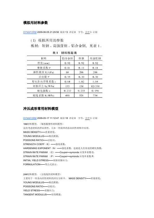
模拟用材料参数DYNAFORM 2009-06-05 21:29:56 阅读13 评论0 字号:大中小订阅冲压成形常用材料模型DYNAFORM 2009-05-17 11:12:47 阅读18 评论0 字号:大中小订阅18#材料模型:(幂指数塑性材料模型)没有考虑材料的厚向异性,只在一些简单的各向同性材料中应用。
MASS DENSITY——质量密度;YOUNG MODULUS——杨氏模量;POISSONS RATIO——泊松比;STRENGTH COEFF(K)——强度系数;HARDENING EXPONENT(N)——强化系数,也就是人们常说的硬化指数;STRAIN RATE PARAM (C)——Couper—symonds应变率系数C;STRAIN RATE PARAM (P)——Couper—symonds应变率系数P;INITIAL YIELD STRESS——初始屈服应力;FORMULATION——用公式表示。
24#材料模型:(分段线性材料模型)主要用于一些各向同性材料的冲压分析中。
MASS DENSITY——质量密度;YOUNG MODULUS——杨氏模量;POISSONS RATIO——泊松比;YIELD STRESS——屈服应力;TANGENT MODULUS——切变模量;FAILURE PL。
STRAIN——材料失效时的等效塑性应变;STEP SIZE FOR EL. DEL——段数;STRAIN RATE PARAM (C)——Couper—symonds应变率系数C;STRAIN RATE PARAM (P)——Couper—symonds应变率系数P;DYNAFORM 基本分析过程DYNAFORM 2009-05-01 18:01:57 阅读58 评论0 字号:大中小订阅这是在一个论坛上看到的,感觉还不错,特别适合于初学者,故在此与大家共同分享。
DYANFORM分析过程介绍一、导入几何或网格模型FILE----IMPORT二、修改零件名称PARTS----EDIT三、划分曲面网格对于坯料:TOOLS----BLANK GENERATOR对于工具:PREPROCESS----ELEMENT四、检查网格PREPROCESS----MODEL CHECK五、创建不见及偏置凹模(凸模)创建凸模(凹模)和压边圈创建部件:PARTS----CREAT偏置单元:PREPROCESS----ELEMENT----COPY六、分离压料面和凸模(凹模)PARTS----ADD TO PART/SEPARATE七、定义坯料材料及属性TOOLS----DEFINE BLANK八、定义工具TOOLS----DEFINE TOOLS九、定义等效拉延筋创建拉延筋线:PREPROCESS----LINE/POINT----FE BOUNDARY LINE/OFFSET创建拉延筋:TOOLS----DRAW BEAD十、工具自动定位分析设置:TOOLS----ANALYSIS SETUP自动定位:TOOLS----POSITION----AUTO POSITION十一、定义工具运动曲线测量工具间距离:TOOLS----POSITION----MIN DISTANCE定义工具运动速度/力曲线:TOOLS----DEFINE TOOLS----DEFINE LOAD CURVE十二、检查工具运动情况TOOLS----ANIMATE十三、定义成形参数和控制参数ANALYSIS----ANALYSIS十四、提交工作到求解器进行计算ANALYSIS----FULL RUN DYNA十五、后处理分析POSTPROCESS十六、分析报告DFE模面设计过程一、导入零件几何模型DFE----PREPARATION----IMPORT二、划分网格1、创建新零件DIEPART----CREAT2、划分网格DFE----PREPARATION----MESH TOOL三、检查并修补网格DFE----MODEL CHECK/REPAIR四、冲压方向调整DFE----TIPPING/UNDERCUT五、内部填充DFE----PREPARATION----INNER FILL六、外部光顺DFE----PREPARATION---OUTER SMOOTH七、创建压料面DFE----BINDER八、创建过渡面(工艺补充面)DFE----ADDENDUM九、切割压料面DFE----MODIFICATION----BINDER TRIMBSE坯料估算过程一、导入零件模型BSE----PREPARATION----IMPORT二、划分网格BSE----PART MESH三、检查和修补网格BSE----MESH CHECK/REPAIR四、坯料尺寸估算BSE----BLANK SIZE ESTIMATE----MSTEP五、坯料网格划分BSE----DEVELOPMENT----BLANK GENERATOR 六、外部光顺BSE----OUTER SMOOTH七、生成新的坯料轮廓线和网格PREPROCESS----LINE/POINT----FE BOUNDARY LINEBSE----DEVELOPMENT----BLANK GENERATOR八、坯料排样BSE----NESTING九、输出排样报告和报价DY中的模拟设置DYNAFORM 2009-04-30 22:06:33 阅读7 评论0 字号:大中小订阅(1)DY中的模拟设置即DY中的“SETUP”菜单,它主要包括两种设置类型:一种为快速设置(QS);一种为自动设置(TUTOSETUP)。
强壮灵合剂的抗炎作用

胃内漂浮滞留型缓释片是依据流体动力学原理,此种剂型进入人体胃环境内,能够漂浮于胃液的上面,并且能够缓慢释放药物,该制剂被称之为“生物有效制剂”[15]。
组成此种剂型的几个因素为药物、亲水凝胶滞留材料以及其他的辅助材料。
在凝胶屏障的保护下,该种剂型的骨架材料的密度小于胃内容物,因此漂浮于胃液之上,并且不受胃排空的影响[15]。
崔京浩[16]等根据胃内滞留剂的释药原理,将葛根素制成胃内滞留剂。
首先将难溶物葛根素制成HP-β-CD 包合物,作为滞留剂的内容物。
以海藻酸钙做为滞留微丸的主要材料,通过考察其他辅料(甲基纤维素、硬脂酸镁、壳聚糖)对药物释放的影响。
实验结果表明,硬脂酸镁为2%时,滞留剂的漂浮效果最好。
与此同时,考察该剂型在人工胃液中的释放情况,其在8h 内的累积释放率为87%,未出现药物突释现象。
胃内滞留丸不仅表现了较好的漂浮效果,其缓释效果也很稳定。
7 小结目前已研究的葛根素缓控释制剂很多,但是从体内药动学的角度来看,关于葛根素制剂的体内研究还不完善,葛根素制剂的体内运行机理还未明确。
希望以上关于葛根素的剂型总结,为以后学者们对葛根素的深入研究提供一定的帮助。
参考文献[1] 夏华玲.葛根素药理作用研究进展[J].时珍国医国药,2006,17(3):434.[13]宋金春,陈佳丽,黄岭.葛根素环糊精包合物脂质体的制备及体外性质研究[J].中国药学杂志,2008,43(23):1792-1797.LIN H S,CHAN S Y,YANGLOW K S.Ki n eti c study of 2 -hydrox yprop y -β-c yc l ode xtr i n-based Formulation of all -tr ansre ti no i c ac i d in sprague -dawle rast after o r a l or i ntr avenousa dmini stra ti o n[J].J Pha r m Sc i,2000,89(2):260-267.Sheth P R,Tossun ia n J L.The hydr odyna mi ca ll y ba l anced system (HBSTM);A nove l dr ug de li ve ry system fo r o r a l use[J].Dr ug D e vInd Pha r m,1984,10(2):313-316.[14][15][16] 崔京浩,钱颖,缪文俊,等.含葛根素-羟丙基β-环糊精包合物胃滞留剂的制备与体外评价[J].中国中药杂志,2008,33(16):1960-1964.收稿日期:2013-08-26强壮灵合剂的抗炎作用李娜1李仁花2窦德强1*姜素云3*1.辽宁中医药大学(大连116000)2 .吉林省图们市人民医院(吉林132000)3.大连市食品药品检验所(大连 116021)[2]苑程鲲,沈文娟,吴效科.葛根素临床应用新进展[J].中医药信息,2011,28(6):125-127. 马家骅,杨明,曹世栋,等.葛根素的提取和含量测定[J].华西药学杂志,2006,21(2):206-207. 由立红,邹英华,景秋芳,等.葛根素缓释复合骨架片理化性质的研究[J].沈阳药科大学学报,2002,19(3):168-172. 景秋芳,任福正,沈永嘉,等.葛根素复合骨架缓释片的处方及制备工艺[J].华东理工大学学报,2003,29(2):173-180. 周珊珊,谭睿,谢彬,等.葛根素骨架缓释片的研制及体外释放评价[J].中国实验方剂学杂志,2013,19(3):23-26. 高秀蓉,许小红,张永模,胡霞.葛根素包衣缓释滴丸的制备及其体外释放度研究[J].时珍国医国药,2011,22(6):1417-1419. 刘伟星,李宁,高崇凯.葛根素自微乳化渗透泵控释胶囊的制备[J].中草药,2013,44(12):1568-1573.摘要目的研究强壮灵合剂对小鼠炎症的影响。
- 1、下载文档前请自行甄别文档内容的完整性,平台不提供额外的编辑、内容补充、找答案等附加服务。
- 2、"仅部分预览"的文档,不可在线预览部分如存在完整性等问题,可反馈申请退款(可完整预览的文档不适用该条件!)。
- 3、如文档侵犯您的权益,请联系客服反馈,我们会尽快为您处理(人工客服工作时间:9:00-18:30)。
a r X i v :g r -q c /9710107v 1 22 O c t 1997Mon.Not.R.Astron.Soc.000,000–000(0000)Printed 7February 2008(MN L A T E X style file v1.4)3+1formulation of non-ideal hydrodynamicsJochen Peitz 1⋆and Stefan Appl 2,3†1LandessternwarteK¨o nigstuhl,69117Heidelberg,Germany 2ObservatoireAstronomique,Universit´e Louis Pasteur,11,rue de l’Universit´e ,67000Strasbourg,France3Institut f¨u r Angewandte Mathematik,Universit¨a t Heidelberg,Im Neuenheimer Feld 294,69120Heidelberg,Germany Accepted for publication in the MNRAS ABSTRACT The equations governing dissipative relativistic hydrodynamics are formu-lated within the 3+1approach for arbitrary spacetimes.Dissipation is ac-counted for by applying the theory of extended causal thermodynamics (Israel-Stewart theory).This description eliminates the causality violating infinite signal speeds present in the conventional Navier-Stokes equation.As an ex-ample we treat the astrophysically relevant case of stationary and axisymmet-ric spacetimes,including the Kerr metric.The equations take a simpler form whenever the inertia due to the dissipative contribution can be neglected.Key words:relativity –hydrodynamics –black hole physics –accretion,accretion discs –galaxies:active –stars:neutron1INTRODUCTIONThe motion of dissipative fluids in strong gravitational fields is of considerable interest in various fields of astrophysics and cosmology.Examples include accretion discs around compact objects,rotating relativistic fluid configurations such as supermassive stars,neutron stars or strange (boson)stars,the collapse of stellar objects and the merging of compact objects.Examples in cosmology cover inflationary cosmological scenarios and the evolution of density fluctuations.The non-stationary modeling of relativistic matter is most conveniently performed within ⋆e-mail:jpeitz@lsw.uni-heidelberg.de†e-mail:appl@gaia.iwr.uni-heidelberg.dec0000RAS2J.Peitz and S.Applthe3+1formalism,where the equations of motion for gravitational-and matterfields are decomposed w.r.t.a congruence offiducial observers(FIDOs),allowing to express time derivatives on a per-unit-universal-time basis.The3+1representation of the equations for ideal,non-dissipative(relativistic)hydrodynamics as well as Maxwell’s equations for the electric and magneticfields and Einstein’s equations for the gravitationalfields have been discussed by many authors,both in a cosmological context(e.g.Durrer&Straumann1988) and in the case of black hole spacetimes(e.g.Thorne&Macdonald1982).Modeling dissipative processes requires non-equilibrium or irreversible thermodynamics. Standard(or classical),irreversible thermodynamics(in the following referred to as standard thermodynamics)wasfirst extended from Newtonian to relativisticfluids by Eckart(1940). However,the Eckart theory,and a variation thereof by Landau&Lifshitz(1959)shares with its Newtonian counterpart serious problems.Notably that dissipativefluctuations propagate at an infinite speed.In addition,generic short wavelength secular instabilities driven by dissipative processes exist(Lindblom&Hiscock1983)andfinally,no well-posed initial value problem exists for rotatingfluid configurations.At the origin of these problems in standard thermodynamics is the description of non-equilibrium via the local equilibrium states alone,i.e.it is assumed that local thermodynamic equilibrium is established on an infinitely short time-scale(see e.g.Jou,Casas-V´a zquez& Lebon1997for an introduction).In extended theories of irreversible thermodynamics the set of thermodynamic variables is extended to include the dissipative variables.This re-stores causality and stability under a wide range of conditions(Hiscock&Lindblom1983).A non-relativistic extended theory was proposed by M¨u ller(1967),and was then general-ized to the relativistic case by Israel(1976)and Stewart(1977).The extended theory is commonly referred to as causal thermodynamics,second-order thermodynamics or transient thermodynamics.The problem of non-causality has recently received attention in the context of transonic accretion discs.Two different approaches have been proposed to overcome this difficulty. For steadyflow Narayan(1992)has established causality by calculating the coefficient of kinematic viscosity within an extended version offlux limited diffusion theory(Levermore& Pomraning1981),assuming a particular steady state phase-space distribution function for the turbulentfluid elements in the disc.The influence of this modified viscosity coefficient was studied in stationary accretion discs by Popham&Narayan(1994)and Syer&Narayan (1993).A relativitic generalization of the modified viscosity has been proposed,and used inc 0000RAS,MNRAS000,000–0003+1formulation of non-ideal hydrodynamics3 models of stationary relativistic accretion discs(Peitz&Appl(1997)).A different approach by Papaloizou&Szuskiewicz(1994),which is related to a causal description for the thermo-dynamics,was used by Kley&Papaloizou(1997)in time-dependent models for accretion disc boundary layers.Gammie&Popham(1997)have recently considered a similar extension to stationary relativistic accretion discs.In cosmology the theory of causal thermodynamics is currently attracting growing interest predominantly in the contexts of re-heating processes after inflation(Zimdahl,Pav´o n&Maartens1997)and in linear perturbation theory for the evolution of densityfluctuations(Maartens&Triginer1997).This paper provides a complete set of equations for dissipativefluid mechanics in their 3+1representation,using a causal description of thermodynamics.In Section2the ba-sic elements of both standard and causal dissipative hydrodynamics are reviewed in their spacetime description,and their3+1representation is derived in Section3.As a particular application of astrophysical interest we specify the system of equations given in Section3 to the case of a stationary,axisymmetric back ground in Section4.2DISSIPATIVE RELATIVISTIC HYDRODYNAMICSThe equations of ideal relativisticfluid mechanics and the equations for dissipative relativis-ticfluid mechanics in both the standard irreversible and the extended causal thermodynam-ics description are reviewed.For a detailed discussion see Israel&Stewart(1979),Hiscock &Lindblom(1983)or a recent treatment by Maartens(1997).2.1NotationWe use geometrized units such that c=1=G.Tensorfields defined on spacetime(M,g) with metric g of signature(−,+,+,+)appear in roman(e.g.u,T),while scalar functions are in italic.The velocity u of thefluid is normalized to u·u=−1.The tensor h=g+u⊗u projects into the3-space orthogonal to u,the local rest frame of thefluid(LRF).Total projections(i.e.projection in any free index)parallel to and orthogonal to u are denoted by()u and()h.If A,B and C are a scalar,vector and rank-2tensorfield on(M,g), respectively,thenA u=A h=A,B u=B u=u·B,B h=h·B,C u=C u=u·C·u,C h=h·C·h.(1) c 0000RAS,MNRAS000,000–0004J.Peitz and S.ApplTwo covariant differential operators˙D and D are defined as projections of the affine con-nection∇on(M,g)into directions parallel and orthogonal to u,˙D≡∇=u·∇,(2)uD≡∇h=h·∇.(3) For2-tensorfields C we further introduce(anti-)symmetrization operators a and s by C= C a if C is anti-symmetric and C= C s if C is symmetric and trace-free.Finally,the irreducible decomposition of∇u yields∇u=σ+ω+1/3Θh−a⊗u,(4) with shearσ≡ ∇u s h,vorticityω≡ ∇u a h,acceleration a≡˙D u and expansionΘ≡D·u=∇·u of thefluid trajectories.2.2PerfectfluidsA perfectfluid is described by the velocity u,baryon number density n,mass-energy density ρ,isotropic pressure p and specific entropy s,which are subject to the conservation laws0=∇·n,(5) 0=∇·T.(6) The particle current vector n and the symmetric stress-energy tensor T are given byn=n u,(7) T=ρu⊗u+p h.(8) The LRF conservation laws for energy and momentum result from projecting(6)parallel and orthogonal to u.With(8)one can write0=(∇·T)u and0=(∇·T)h as0=˙Dρ+(ρ+p)Θ,(9) 0=D p+(ρ+p)a.(10) The metric g is coupled to stress-energy T by Einstein’s equationsG=8πT,(11) where G is the Einstein tensor.Thermodynamic scalar functions are defined in the LRF.The entropyfluxs=s n(12)c 0000RAS,MNRAS000,000–0003+1formulation of non-ideal hydrodynamics5 is conserved alongflow lines(adiabaticflow),0=∇·s.(13) The temperature T is defined via the Gibbs equationT d s=d(ρ/n)+p d(1/n),(14) where d is the exterior derivative on(M,g).In general,two thermodynamic scalars are needed as independent variables,which we choose n andρ.A scalar equation of state,e.g. p=p(n,ρ),closes the system of equations(5),(9)-(11)for the dynamical variables{n,ρ,u, g}.2.3DissipativefluidsChoosing the particle current for dissipativefluids by(7)corresponds to selecting an average velocity u such that the particleflux in the associated rest frame vanishes.This so-called particle frame or Eckart frame(Eckart1940)is the natural frame in systems where particle number is conserved(see Israel&Stewart1979for the alternative energy frame description). The state of thefluid is assumed close to afictitious thermodynamic equilibrium state, characterized by the local thermodynamic equilibrium scalars n0,ρ0,p0,s0,T0and the local equilibrium velocity u0,which in the Eckart frame can be chosen such that only the pressure p deviates from the local equilibrium pressure p0by the bulk viscous pressureΠ=p−p0, whereas n=n0andρ=ρ0.Dropping subscripts0allows then to write the general stress-energy tensor for dissipativefluids asT=ρu⊗u+(p+Π)h+q⊗u+u⊗q+π,(15) where the heatflux q relative to the particle frame and the anisotropic stress tensorπare orthogonal to u,q=q h,π= π s h.(16) Conservation laws again hold for n and T.However,in irreversible thermodynamics the entropy is no longer conserved.According to the second law,the rate of entropy generation must therefore be positive definite,∇·s≥0,(17) implying that s has a dissipative vector contribution R in excess to(12),s=s n+R/T.(18) c 0000RAS,MNRAS000,000–0006J.Peitz and S.ApplFollowing the phenomenological Israel-Stewart approach,s=s0remains related to T=T0 by the Gibbs equation(14).The dissipative part R is assumed to be an algebraic function of n and T only,which vanishes in equilibrium(R0=0).The theories of standard irreversible thermodynamics and of extended causal thermodynamics differ in the forms of R,as given below.The equations of energy and momentum conservation for(15)can be written as0=˙Dρ+(ρ+p+Π)Θ+σ:π+(2a+D)·q,(19) 0=(ρ+p+Π)a+D(p+Π)+D·π+π·a+(˙D q)h+(σ+ω+4/3Θh)·q(20) where B:C≡tr(B·C)for2-tensorfields B,C.The above treatment applies for a single-componentfluid and allows a natural extension to multi-componentfluids.2.4Standard thermodynamicsStandard thermodynamics assumes a linear dependence of R on the thermodynamicfluxes {Π,q,π},which is possible only if(18)takes the forms=s n+q/T.(21) Using(5),(19)and(20)yields the entropy generation rateT∇·s=−ΘΠ−(D ln T+a)·q−σ:π.(22) The simplest relation to be imposed between the thermodynamicfluxes{Π,q,π}and the thermodynamic forces{3Θ,D ln T+a,σ}in agreement with(17)is linear,Π=−ζΘ,(23) q=−λT(D ln T+a),(24)π=−2ησ,(25) with non-negative coefficients of bulk viscosityζ(ρ,n),thermal conductivity,λ(ρ,n)and shear viscosityη(ρ,n).This brings(22)toT∇·s=Π2/ζ+q·q/(λT)+π:π/(2η),(26) which on using(5),(14),(19)and(20)yields an evolution equation for the entropy density s,T n˙Ds=−ΘΠ−∇·q−a·q−π:σ.(27)c 0000RAS,MNRAS000,000–0003+1formulation of non-ideal hydrodynamics7 As a consequence of(23)-(25),the thermodynamicfluxes react instantaneously to the cor-responding thermodynamic forces,implying propagation of signals at(causality violating) infinite speed.In standard thermodynamics thedynamics of thefluid is governed by the(com-pressible)Navier-Stokes equation,which results from substitution of(23)-(25)into(20).2.5Causal thermodynamicsKinetic theory can motivate that R is second-order in the dissipative terms(Israel&Stewart 1979).Truncation atfirst order removes terms necessary for causality and stability.The most general algebraic form for R of at most second-order in the dissipativefluxes leads tos=s n+q/T−1/2 β0Π2+β1q·q+β2π:π u/T+α0Πq/T+α1π·q/T.(28) The entropy density measured in LRF then becomes−s·u=sn−1/2 β0Π2+β1q·q+β2π:π .(29) The negative sign of the non-equilibrium contributions reflects the fact that the entropy den-sity is maximum in equilibrium.The thermodynamic coefficientsβj(ρ,n)≥0in(28)model deviations of the physical entropy density from sn due to scalar/vector/tensor dissipative contributions to R.Theαi(ρ,n)model contributions due to viscous/heat coupling,which do not influence the physical entropy density(29).The entropy generation rate associated with(28)follows from(5),(14),(19)and(20)to T∇·s=−ΠX−q·Y−π: Z s(30) with the scalar,vector and rank-2tensorfieldsX=Θ+β0˙DΠ−α0D·q−κ0T q·∇(α0/T)+1/2ΠT∇·(β0u/T),(31) Y=∇ln T+a+β1˙D q−α0∇Π−α1∇·π−(1−κ0)ΠT∇(α0/T)−(1−κ1)Tπ·∇(α1/T)+1/2T q∇·(β1u/T),(32) Z=∇u+β2˙Dπ−α1∇q−κ1T q⊗∇(α1/T)+1/2Tπ∇·(β2u/T).(33) The simplest evolution equations for the causal thermodynamicfluxes{Π,q,π}in agreement with the second law(17)are again linear relationships,Π=−ζX,(34) q=−λT Y h,(35)π=−2η Z s.(36)hc 0000RAS,MNRAS000,000–0008J.Peitz and S.ApplTwo additional thermodynamic coefficientsκk(ρ,n)had to be introduced in(31)-(33)as a consequence of the ambiguity involved in factoring terms which involve productsΠq and π·q in(28).Furthermore,(34)-(36)contain terms involving gradients of theαi andβj. Since theκk are unknown a priori,these terms could be important even if the gradients themselves are small(Hiscock&Lindblom1983).Finally,in(31)-(33)we neglected further contributions due to additional coupling terms between{Π,q,π}and a,ω,which can be shown to exist in kinetic theory(Israel&Stewart1979).The complexity of the full evolution equations(34)-(36)makes applications tractable only if certain simplifications are made.A particularly simple set of evolution equations results from the assumptions(Maartens1997)0=κ0=κ1,(37) 0=α0=α1,(38) 0≃∇·(βj u/T),(39) where(37)reflects essentially the lack of knowledge on theκk while(38)neglects the cou-pling between heatflux and viscosity.Implications of(39)are multifold and need to be justified after a particular solution was found using a parametrization forβj(ρ,n).The evo-lution equations resulting from(34)-(36)under the assumptions(37)-(39)are of covariant relativistic Maxwell-Cattaneo form,τ0(˙DΠ)h+Π=˜Π,(40)τ1(˙D q)h+q=˜q,(41)τ2(˙Dπ)h+π=˜π,(42) with the relaxation timesτj(ρ,n)given byτ0=ζβ0,τ1=λTβ1,τ2=2ηβ2,,(43) and{˜Π,˜q,˜π}the(re-named)standard thermodynamicfluxes as in(23)-(25).In contrast to the algebraic constraint equations(23)-(25),the evolution equations(40)-(42)arefirst order partial differential equations,which assure that in the LRF the viscous bulk/shear stresses and the heatflux relax towards their standard limits{˜Π,˜q,˜π}on time-scalesτj. The relaxation timesτj follow in principle from kinetic theory,but can be estimated as mean collision times,1/τ∼nΣv,withΣthe collision cross section and v the mean particle speed.c 0000RAS,MNRAS000,000–0003+1formulation of non-ideal hydrodynamics 9For later use we re-write (40)-(42)as˙DΠ=1τ1˜q −q +(q ·a)u ,(45)˙D π=1=−ζΘ=−λT D ln T ,(48)˜π,(49)with the thermodynamic forces calculated from the kinematic propertiesΘ≡a |a=0=0,σh .(50)The causal evolution equations (44)-(46)simplify to˙DΠτ0˜Π ,(51)˙D q τ1˜q ,(52)c 0000RAS,MNRAS 000,000–00010J.Peitz and S.Appl˙Dπτ2 ˜π .(53)3DISSIPATIVE HYDRODYNAMICS IN3+1FORMULATION Particularly useful for time-dependent calculations in general relativity is the3+1formu-lation,where time derivatives are always with respect to globally defined universal time. Applications of3+1hydrodynamics and3+1magnetohydrodynamics have been mostly re-stricted to idealfluids(see Bonazzola et al.1993for an exception).A collection of numerous general relativistic equations in the3+1representation can be found in Durrer&Straumann (1988).We give a3+1representation of relativistic dissipative hydrodynamics for both,stan-dard and causal thermodynamics.For a detailed derivation of the equations presented in this section we refer to Peitz(Peitz1998).3.1Generalities on the3+1formalismAssuming that spacetime(M,g)admits a slicing by slicesΣt,i.e.there is a diffeomorphism Φ:M→Σ×I,I⊂I R,such that the manifoldsΣt=Φ−1(Σ×{t})are spacelike and the curvesΦ−1(m,t)are timelike.These curves define a vectorfield∂t which can be decomposed into normal and parallel components relative to the slicing,∂t=αˆn+β.(54) Hereˆn is the timelike unit normalfield(congruence offiducial observers=FIDOs)andβis tangent to the slicesΣt.αis the lapse function andβis the shift vectorfield.A coordinate system{x i}onΣinduces natural coordinates on M,i.e.Φ−1(m,t)has coordinates(t,x i)if m∈Σhas coordinates x i.The timelike curves∂t have constant spatial coordinates (preferred timelike curves).Now setβ=βi∂i(where∂i≡∂/∂x i).From g(ˆn,∂i)=0one finds g(∂t,∂t)=−(α2−βiβi)and g(∂t,∂i)=βi.In coordinates co-moving with the FIDOs the metric thus readsg=−(α2−βiβi)d t⊗d t+βi d t⊗d x i+βi d x i⊗d t+γij d x i⊗d x j(55) =−α2d t⊗d t+γij(d x i+βi d t)⊗(d x j+βj d t).(56) The forms d t and d x i+βi d t are thus orthogonal.γis the metric induced onΣt,and the affine connection on(Σt,γ)is denoted by∇.The tangent and cotangent spaces of M have two natural decompositions,which give rise to two types of bases of vectorfields and1-forms.These are the dual pair{∂µ}andc 0000RAS,MNRAS000,000–000{d xµ}for comoving coordinates{xµ}and,on the other hand,the dual pair{ˆn,∂i}and {αd t,d x i+βi d t}.Instead of the coordinate basis{∂i}one may also use an orthonormal horizontal basis{e i}with g(e i,e j)=δij,together with the dual basis{ϑj}for{d x i}.Then one has the two dual pairs{∂t,e i},{d t,ϑi}and{e0=ˆn,e i},{θµ}with the orthonormal tetrad{θµ}given byθ0=αd t andθi=ϑi+βi d t,withβi defined byβ=βi e i.From(54) follows the relation1e0=ˆn=on(Σt,γ),and the horizontal parts of only two spatial tensorfields,namelyˆa=∇lnα,(61) K=TK.(62) Here K is the extrinsic curvature tensor(second fundamental form),defined on(M,g)by K≡−∇ˆn=−13ˆΘγ+1α ∂t−Lβ E A+˙D E A,(65)E ˙D B =γα ∂t−LβS B+˙D S B−E B F−γK·S B,(67)E ˙D C =γα ∂t−LβS C+˙D S C−γK·T C− E Cγ+T C ·F,(69)T ˙D C =γirreducible decomposition∇u=σ+ω+1α ∂t−Lβ(γn)+1α ∂t−Lβ E T−tr(K)E T+2(S T·∇)lnα+∇·S T−tr(K·T T),(80)0=1α∇·(αTT).(81)For completeness we give the3+1representation of the Einstein equations(e.g.Durrer c 0000RAS,MNRAS000,000–000&Straumann1988).They consist of evolution equations forγand K,obtained from the definition of the extrinsic curvature(63)and from the(space,space)components of(11). These dynamical equations arefirst order differential equations,1α ∂t−Lβ K=Ri(γ)−2K2+tr(K)K−8πT T+4π tr(K)−E T γ−He(lnα),(83)where K2≡K·K,Ri()is the Ricci tensor and He()is the Hessian on(Σt,γ),respectively. The(time,time)and(time,space)components of(11)yield the Hamiltonian and momentum constraints,R−tr(K)2−tr(K2)=16πE T,(84)∇·K−∇tr(K)=8πST,(85) where R is the curvature scalar on(Σt,γ).3.3The standard constraint equationsThe3+1representation of the constraint equations(23)-(25)for the thermodynamicfluxes {˜Π,˜q,˜π}depends on the3+1representation of the kinematic propertiesΘ,a,σof thefluid, which can be calculated toEΘ=W+ϑ−γtr(K),(86)Ea=γW+˙Dγ−K u,(87)Sa=γW+a,(88)E σ=12(γ2−1)W+γ2 Dγ+γa − 12(γ2−1)W+13 W+ϑ−γtr(K) u− 12 W⊗u+u⊗W−1α ∂t−Lβγ+(u·∇)lnα,(92)W≡1(23)-(25),E ˜Π=−ζEΘ,(94)E˜q=−λT γ2−1 1α ∂t−Lβ ln T+D ln T+S a ,(96)E ˜π=−2ηEσ,(97)S ˜π=−2ηSσ,(98)T ˜π=−2ηTσ.(99)3.4The causal evolution equationsFor the sake of simplicity the following discussion will be restricted to the causal evolu-tion equations(44)-(46).Generalization to the full evolution equations(34)-(36)is straight-forward.The required3+1representations of˙DΠ,˙D q,˙Dπfollow readily from(65)-(70). Remains to decompose products q·a in(45)andπ·a in(46),E q·a =EqEa+Sq·S a,(100)E π·a =EπEa+Sπ·S a,(101)S π·a =EaSπ+Tπ·S a.(102)The3+1evolution equations for the causal thermodynamicfluxes{EΠ,E q,S q,Eπ,Sπ,Tπ} then follow from(44)-(46)toγτ0 E˜Π−EΠ ,(103)γτ1 E˜q−E q +γE q·a+F·S q,(104)γτ1 S˜q−S q +E q·a u+E q F+γK·S q,(105)γτ2 E˜π−Eπ +2γEπ·a+2F·Sπ,(106)γτ2 S˜π−Sπ +γSπ·a+Eπ·a u+γK·Sπ+ Eπγ+Tπ ·F,(107)γτ2 T˜π−Tπ +u⊗Sπ·a+Sπ·a⊗u+2γK·Tπ+F⊗Sπ+Sπ⊗F,(108)with F according to(71).c 0000RAS,MNRAS000,000–0003.5The weakly dissipative limitThe limit of weak dissipation discussed in section 2.6implies three simplifications of the 3+1equations of causal hydrodynamics.The first simplfication concerns the 3+1conservation laws (80)and (81)for energy and momentum,where dissipative contributions {Π,q,π}to the matter sources {E T ,S T ,T T }in (75)-(78)can be dropped wherever they enter alge-braically,and only temporal and spatial gradients remain.The second simplification affects the 3+1representation of the kinematic properties of the fluid,(86)-(91).Using the geodesic conditions E a =S a =0,(87)and (88)yield simplified expressions for W and W ,W =−˙D ln γ+K u /γ,(109)W =−a /γ,(110)which are no longer time-dependent.Therefore,any kinematic properties (86)-(91)simplify to time-independent expressionsΘE =0,(112)aE =13γ2−1ϑ−γtr(K )=23ϑ−γtr(K ) +1S =13˙D ln γ−K u /γ−ϑ+γtr(K ) γu ,(115)σ−γK +1= ∇u s −1/2ϑh .Finally,the weak dissipation limit affects the 3+1evolution equa-tions (103)-(108)for the thermodynamic fluxes {E Π,E q ,S q ,E π,S π,T π},where productsE q ·a ,E π·a ,S π·a as in (100)-(102)are dropped.This yields the weak dissipative evolution equations for the thermodynamic fluxes {E Π,S q ,S π},γ+˙D E Πτ0 E ˜Π ,(117)γ+˙D E q τ1 E ˜q +F ·S q α ∂t −L β S q =1−S q F +γK ·S q α ∂t −L β E π=1−E π,(120)c0000RAS,MNRAS 000,000–000γ+˙D Sπτ2 S˜π +γK·Sπγ+Tπα ∂t−Lβ Tπ=1−Tπ+F⊗Sπ⊗F.(122)4STATIONARY AND AXISYMMETRIC BACKGROUND SPACETIMES The3+1equations of dissipative hydrodynamics are specified to the class of stationary,ax-isymmetric background spacetimes.This situation is realized if thefluid under consideration has negligible influence on the gravitationalfield of a central object,and in addition this field is known to be stationary and axisymmetric.These assumptions include most appli-cations related to accretion/ejectionflows in the vicinity of compact objects.For rotating black holes the vacuum metric is Kerr,and we give the equations also for this special case.4.1Implications of symmetriesThe general form of a stationary,axisymmetric vacuum spacetime can be put in a form which is symmetric under a simultaneous change of sign of t andφ,the Killing coordinates associated with the commuting time and axial Killing vectorfields k and m.Choosing the remaining two meridional coordinates as spherical coordinates allows to write g asg=−α2d t⊗d t+˜ω2(dφ−ωd t)⊗(dφ−ωd t)+e2µd r⊗d r+e2νdθ⊗dθ,(123) with the invariant metric coefficients˜ω2=m2,ω=−k·m/m2,α2=−k2+k·m/m2.(124) For the physical interpretation of˜ω,ωandαsee e.g.Bardeen(1970).The generic choice of thefiducial congruence is(see e.g.Thorne&Macdonald(1982)for criteria that uniquelyfix this choice)ˆn=e0=1and the metric induced on (Σt ,γ)becomes γ=˜ω2d φ⊗d φ+e 2µd r ⊗d r +e 2νd θ⊗d θ.(127)The 3+1representation of Killing’s equation for k and m,together with their commutivity,allows to establish the following relations (Thorne &Macdonald 1982)∂t µ=0,∂t ν=0,∂t ω=0,∂t m =0,∂t γ=0,(128)m ·∇µ=0,m ·∇ν=0,m ·∇ω=0, ∇m s =0,(129)ˆΘ=0,ˆσ=12αm ⊗∇ω+∇ω⊗m .(131)Therefore K measures the shear of hypersurfaces Σt ,which vanishes for ω=0.4.2Gravitomagnetic and gravitoelectric tensor fieldsA characteristic phenomenon in axisymmetric spacetimes is the dragging of inertial frames.Physical implications due to this effect (see Thorne et al.1986for the case of the Kerr metric)are often described in terms of the gravitomagnetic tensor field H ,defined on (Σt ,γ)by H ≡1α∇(ωm )=−12(H ·T +T ·H ).(133)The antisymmetric part of H can be expressed as an axial vector field on (Σt ,γ),namely the gravitomagnetic vector field J ≡12J ∧S .(135)The Lie derivatives L βin the 3+1equations derived in section 3can then be expressed as L βE =(β·∇)E ,(136)L βS =(β·∇)S −(S ·∇)β=(β·∇)S −αS ·H ,(137)c0000RAS,MNRAS 000,000–000LβT=(β·∇)T−2 (T·∇)β s=(β·∇)T−2α T·H s=(β·∇)T−2T·K.(138) The term S·H in(137)may be expressed by either H as in(132)or in terms of J and K via(135).In addition to the gravitomagnetic tensorfields H and J,we introduce the gravitoelectric vectorfield G,defined on(Σt,γ)byG≡−ˆa=−∇lnα.(139) Thisfield measures the gravitational acceleration measured by thefiducial observers.4.3Conservation lawsThe3+1conservation laws for particle number(79),energy(80)and momentum(81)in a stationary,axisymmetric background read0=1∂t−β·∇(γn)+1α ∂α ∂α∇(αT T)=1∂t−β·∇S T+∇·T T−H·S T− E Tγ+T T ·G.(142)4.4Evolution equationsThe3+1representation(86)-(91)of the kinematic properties of thefluid in stationary, axisymmetric background readEΘ=W+ϑ,(143)Ea=γW+˙Dγ+ˆσu,(144)Sa=γW+a,(145)E σ=32 γ2−1 W+γ2Dγ+γa − ˆσuγ+ˆσ ·u,(147)T σ=γ3W h+σ+γˆσ(148)with time derivatives contained inW=1∂t−β·∇γ−G u,(149)W=1∂t−β·∇u−H·u−γG.(150)c 0000RAS,MNRAS000,000–000The 3+1representation of the standard constraint equations (94)-(99)can be written as E ˜Π=−ζE Θ,(151)E ˜q =−κTγ2−11∂t −β·∇ ln T +γ˙D ln T +E a ,(152)S ˜q =−κT γu1∂t −β·∇ln T +D ln T +S a ,(153)E ˜π=−2ηE σ,(154)S ˜π=−2ηS σ,(155)T ˜π=−2ηT σ.(156)The 3+1representation ofthe causal evolution equations (103)-(108)reads γ∂t −β·∇E Π+˙DE Π=1α∂τ1E ˜q −Eq+γE q ·a+F ·S q,(158)γ∂t −β·∇S q +˙DS q=12γJ ∧S q,(159)γ∂t −β·∇E π+˙DE π=1α ∂τ2 S ˜π−S π+γS π·a +E π·au +1α ∂τ2T ˜π−T π+u ⊗S π·a+S π·a⊗u +γF ⊗S π+γS π⊗F ,(162)withF =γG −ˆσ·u .(163)4.5Weakly dissipative limitThe 3+1representation of the kinematic properties of the fluid in the weak dissipation limit can be written asΘE =0,(165)aE =13γ2−1ϑ=23ϑ+1σ2 a /γ+∇γ +ˆσ·u +1T =σ3˙D ln γ−ˆσu /γ h .(169)The 3+1weak dissipation evolution equations (103)-(108)for {E Π,S q ,S π}can be written asγ∂t−β·∇ E Π=1−E Πα ∂+˙D E q τ1 E ˜q +F ·S q α ∂+˙D S q τ1S ˜q +E q 2γJ ∧S q α ∂+˙D E πτ2E ˜π +2F ·S πα ∂+˙D S πτ2S ˜π +1+ E π ·F ,(174)γ∂t −β·∇ T π=1−T π+S π∆Σ2,˜ω=Σ∆,e 2ν=̺2.(177)A consistent treatment of viscous hydrodynamics in the vicinity of a rotating black hole would require a careful analysis of the boundary conditions at the horizon.Such an analysis is best performed within the concept of a streched horizon ,defined by a small value of lapse α.We refer to the membrane paradigma of Thorne et al.(1986),where this approach is applied to ideal magnetohydrodynamics and Maxwell’s equations.This work also contains a coordinate representation of G and H .。