15-A family of skew-symmetric-Laplace distributions
翻译的外文文献
The Beginning of Model Checking:A Personal PerspectiveE.Allen Emerson1,21.Department of Computer Sciencesputer Engineering Research CenterThe University of Texas at Austin,Austin TX78712,USAAbstract.Model checking provides an automated method for verify-ing concurrent systems.Correctness specifications are given in tempo-ral logic.The method hinges on an efficient andflexible graph-theoreticreachability algorithm.At the time of its introduction in the early1980’s,the prevailing paradigm for verification was a manual one of proof-theoretic reasoning using formal axioms and inference rules oriented to-wards sequential programs.The need to encompass concurrent programs,the desire to avoid the difficulties with manual deductive proofs,and thesmall model theorem for temporal logic motivated the development ofmodel checking.Keywords:model checking,model-theoretic,synthesis,history,origins1IntroductionIt has long been known that computer software programs,computer hardware designs,and computer systems in general exhibit errors.Working programmers may devote more than half of their time on testing and debugging in order to increase reliability.A great deal of research effort has been and is devoted to developing improved testing methods.Testing successfully identifies many significant errors.Yet,serious errors still afflict many computer systems including systems that are safety critical,mission critical,or economically vital.The US National Institute of Standards and Technology has estimated that programming errors cost the US economy$60B annually[Ni02].Given the incomplete coverage of testing,alternative approaches have been sought.The most promising approach depends on the fact that programs and more generally computer systems may be viewed as mathematical objects with behavior that is in principle well-determined.This makes it possible to specify using mathematical logic what constitutes the intended(correct)behavior.Then one can try to give a formal proof or otherwise establish that the program meets This work was supported in part by National Science Foundation grants CCR-009-8141&CCR-020-5483and funding from Fujitsu Labs of America. email:emerson@ URL:/∼emerson/its specification.This line of study has been active for about four decades now. It is often referred to as formal methods.The verification problem is:Given program M and specification h determine whether or not the behavior of M meets the specification h.Formulated in terms of Turing Machines,the verification problem was considered by Turing[Tu36]. Given a Turing Machine M and the specification h that it should eventually halt (say on blank input tape),one has the halting problem which is algorithmically unsolvable.In a later paper[Tu49]Turing argued for the need to give a(manual) proof of termination using ordinals,thereby presaging work by Floyd[Fl67]and others.The model checking problem is an instance of the verification problem.Model checking provides an automated method for verifying concurrent(nominally)finite state systems that uses an efficient andflexible graph search,to determine whether or not the ongoing behavior described by a temporal property holds of the system’s state graph.The method is algorithmic and often efficient because the system isfinite state,despite reasoning about infinite behavior.If the answer is yes then the system meets its specification.If the answer is no then the system violates its specification;in practice,the model checker can usually produce a counterexample for debugging purposes.At this point it should be emphasized that the verification problem and the model checking problem are mathematical problems.The specification is for-mulated in mathematical logic.The verification problem is distinct from the pleasantness problem[Di89]which concerns having a specification capturing a system that is truly needed and wanted.The pleasantness problem is inherently pre-formal.Nonetheless,it has been found that carefully writing a formal specifi-cation(which may be the conjunction of many sub-specifications)is an excellent way to illuminate the murk associated with the pleasantness problem.At the time of its introduction in the early1980’s,the prevailing paradigm for verification was a manual one of proof-theoretic reasoning using formal axioms and inference rules oriented towards sequential programs.The need to encom-pass concurrent programs,and the desire to avoid the difficulties with manual deductive proofs,motivated the development of model checking.In my experience,constructing proofs was sufficiently difficult that it did seem there ought to be an easier alternative.The alternative was suggested by temporal logic.Temporal logic possessed a nice combination of expressiveness and decidability.It could naturally capture a variety of correctness properties, yet was decidable on account of the“Small”Finite Model Theorem which en-sured that any satisfiable formula was true in somefinite model that was small. It should be stressed that the Small Finite Model Theorem concerns the satisfi-ability problem of propositional temporal logic,i.e.,truth in some state graph. This ultimately lead to model checking,i.e.,truth in a given state graph.The origin and development of model checking will be described below.De-spite being hampered by state explosion,over the past25years model checking has had a substantive impact on program verification efforts.Formal verification2has progressed from discussions of how to manually prove programs correct to the routine,algorithmic,model-theoretic verification of many programs.The remainder of the paper is organized as follows.Historical background is discussed in section2largely related to verification in the Floyd-Hoare paradigm; protocol verification is also considered.Section3describes temporal logic.A very general type of temporal logic,the mu-calculus,that defines correctness in terms offixpoint expressions is described in section4.The origin of model checking is described in section5along with some relevant personal influences on me.A discussion of model checking today is given in section6.Some concluding remarks are made in section7.2Background of Model CheckingAt the time of the introduction of model checking in the early1980’s,axiomatic verification was the prevailing verification paradigm.The orientation of this paradigm was manual proofs of correctness for(deterministic)sequential pro-grams,that nominally started with their input and terminated with their out-put.The work of Floyd[Fl67]established basic principles for proving partial correctness,a type of safety property,as well as termination and total correct-ness,forms of liveness properties.Hoare[Ho69]proposed an axiomatic basis for verification of partial correctness using axioms and inference rules in a formal deductive system.An important advantage of Hoare’s approach is that it was compositional so that the proof a program was obtained from the proofs of its constituent subprograms.The Floyd-Hoare framework was a tremendous success intellectually.It en-gendered great interest among researchers.Relevant notions from logic such as soundness and(relative)completeness as well as compositionality were in-vestigated.Proof systems were proposed for new programming languages and constructs.Examples of proofs of correctness were given for small programs.However,this framework turned out to be of limited use in practice.It did not scale up to“industrial strength”programs,despite its merits.Problems start with the approach being one of manual proof construction.These are formal proofs that can involve the manipulations of extremely long logical formulae. This can be inordinately tedious and error-prone work for a human.In practice, it may be wholly infeasible.Even if strict formal reasoning were used throughout, the plethora of technical detail could be overwhelming.By analogy,consider the task of a human adding100,000decimal numbers of1,000digits each.This is rudimentary in principle,but likely impossible in practice for any human to perform reliably.Similarly,the manual verification of100,000or10,000or even 1,000line programs by hand is not feasible.Transcription errors alone would be prohibitive.Furthermore,substantial ingenuity may also be required on the part of the human to devise suitable assertions for loop invariants.One can attempt to partially automate the process of proof construction using an interactive theorem prover.This can relieve much of the clerical burden.3However,human ingenuity is still required for invariants and various lemmas. Theorem provers may also require an expert operator to be used effectively.Moreover,the proof-theoretic framework is one-sided.It focuses on providing a way to(syntactically)prove correct programs that are genuinely(semantically) correct.If one falters or fails in the laborious process of constructing a proof of a program,what then?Perhaps the program is really correct but one has not been clever enough to prove it so.On the other hand,if the program is really incorrect,the proof systems do not cater for proving incorrectness.Since in practice programs contain bugs in the overwhelming majority of the cases,the inability to identify errors is a serious drawback of the proof-theoretic approach.It seemed there ought to be a better way.It would be suggested by temporal logic as discussed below.Remark.We mention that the term verification is sometimes used in a specific sense meaning to establish correctness,while the term refutation(or falsification) is used meaning to detect an error.More generally,verification refers to the two-sided process of determining whether the system is correct or erroneous.Lastly,we should also mention in this section the important and useful area of protocol work protocols are commonlyfinite state.This makes it possible to do simple graph reachability analysis to determine if a bad state is accessible(cf.[vB78],[Su78]).What was lacking here was aflexible and expres-sive means to specify a richer class of properties.3Temporal LogicModal and temporal logics provided key inspiration for model checking.Origi-nally developed by philosophers,modal logic deals with different modalities of truth,distinguishing between P being true in the present circumstances,pos-sibly P holding under some circumstances,and necessarily P holding under all circumstances.When the circumstances are points in time,we have a modal tense logic or temporal logic.Basic temporal modalities include sometimes P and always P.Several writers including Prior[Pr67]and Burstall[Bu74]suggested that temporal logic might be useful in reasoning about computer programs.For in-stance,Prior suggested that it could be used to describe the“workings of a digital computer”.But it was the seminal paper of Pnueli[Pn77]that made the crit-ical suggestion of using temporal logic for reasoning about ongoing concurrent programs which are often characterized as reactive systems.Reactive systems typically exhibit ideally nonterminating behavior so that they do not conform to the Floyd-Hoare paradigm.They are also typically non-deterministic so that their non-repeatable behavior was not amenable to testing. Their semantics can be given as infinite sequences of computation states(paths) or as computation trees.Examples of reactive systems include microprocessors, operating systems,banking networks,communication protocols,on-board avion-ics systems,automotive electronics,and many modern medical devices.4Pnueli used a temporal logic with basic temporal operators F(sometimes) and G(always);augmented with X(next-time)and U(until)this is today known as LTL(Linear Time Logic).Besides the basic temporal operators applied to propositional arguments,LTL permitted formulae to be built up by forming nestings and boolean combinations of subformulae.For example,G¬(C1∧C2) expresses mutual exclusion of critical sections C1and C2;formula G(T1⇒(T1U C1)specifies that if process1is in its trying region it remains there until it eventually enters its critical section.The advantages of such a logic include a high degree of expressiveness permit-ting the ready capture of a wide range of correctness properties of concurrent programs,and a great deal offlexibility.Pnueli focussed on a proof-theoretic approach,giving a proof in a deductive system for temporal logic of a small example program.Pnueli does sketch a decision procedure for truth overfinite state graphs.However,the complexity would be nonelementary,growing faster than anyfixed composition of exponential functions,as it entails a reduction to S1S,the monadic Second order theory of1Successor,(or SOLLO;see be-low).In his second paper[Pn79]on temporal logic the focus is again on the proof-theoretic approach.I would claim that temporal logic has been a crucial factor in the success of model checking.We have one logical framework with a few basic temporal operators permitting the expression of limitless specifications.The connection with natural language is often significant as well.Temporal logic made it possible, by and large,to express the correctness properties that needed to be expressed. Without that ability,there would be no reason to use model checking.Alternative temporal formalisms in some cases may be used as they can be more expressive or succinct than temporal logic.But historically it was temporal logic that was the driving force.These alternative temporal formalisms include:(finite state)automata(on infinite strings)which accept infinite inputs by infinitely often entering a desig-nated set of automaton states[Bu62].An expressively equivalent but less succinct formalism is that ofω-regular expressions;for example,ab cωdenotes strings of the form:one a,0or more b s,and infinitely many copies of c;and a property not expressible in LTL(true P)ωensuring that at every even moment P holds. FOLLO(First Order Language of Linear Order)which allows quantification over individual times,for example,∀i≥0Q(i);and SOLLO(Second Order Language of Linear Order)which also allows quantification over sets of times corresponding to monadic predicates such as∃Q(Q(0)∧∀i≥0(Q(i)⇒Q(i+1)).1These alterna-tives are sometimes used for reasons of familiarity,expressiveness or succinctness. LTL is expressively equivalent to FOLLO,but FOLLO can be nonelementarily more succinct.This succinctness is generally found to offer no significant practi-cal advantage.Moreover,model checking is intractably(nonelementarily)hard for FOLLO.Similarly,SOLLO is expressively equivalent toω−regular expres-sions but nonelementarily more succinct.See[Em90]for further discussion.1Technically,the latter abbreviates∃Q(Q(0)∧∀i,j≥0(i<j∧¬∃k(i<k<j))⇒(Q(i)⇒Q(j)).5Temporal logic comes in two broad styles.A linear time LTL assertion h is interpreted with respect to a single path.When interpreted over a program there is an implicit universal quantifications over all paths of the program.An assertion of a branching time logic is interpreted over computation trees.The universal A (for all futures)and existential E(for some future)path quantifiers are important in this context.We can distinguish between AF P(along all futures,P eventually holds and is thus inevitable))and EF P(along some future,P eventually holds and is thus possible).One widely used branching time logic is CTL(Computation Tree Logic)(cf. [CE81]).Its basic temporal modalities are A(for all futures)or E(for some fu-ture)followed by one of F(sometime),G(always),X(next-time),and U(until); compound formulae are built up from nestings and propositional combinations of CTL subformulae.CTL derives from[EC80].There we defined the precursor branching time logic CTF which has path quantifiers∀fullpath and∃fullpath, and is very similar to CTL.In CTF we could write∀fullpath∃state P as well as ∃fullpath∃state P These would be rendered in CTL as AF P and EF P,respec-tively.The streamlined notation was derived from[BMP81].We also defined a modal mu-calculus FPF,and then showed how to translate CTF into FPF. The heart of the translation was characterizing the temporal modalities such as AF P and EF P asfixpoints.Once we had thefixpoint characterizations of these temporal operators,we were close to having model checking.CTL and LTL are of incomparable expressive power.CTL can assert the existence of behaviors,e.g.,AGEF start asserts that it is always possible to re-initialize a circuit.LTL can assert certain more complex behaviors along a computation,such as GF en⇒F ex relating to fairness.(It turns out this formula is not expressible in CTL,but it is in“FairCTL”[EL87])The branching time logic CTL*[EH86]provides a uniform framework that subsumes both LTL and CTL,but at the higher cost of deciding satisfiability.There has been an ongoing debate as to whether linear time logic or branching time logic is better for program reasoning(cf.[La80],[EH86],[Va01]).Remark.The formal semantics of temporal logic formulae are defined with respect to a(Kripke)structure M=(S,S0,R,L)where S is a set of states,S0 comprises the initial states,R⊆S×S is a total binary relation,and L is a labelling of states with atomic facts(propositions)true there.An LTL formula h such as F P is defined over path x=t0,t1,t2...through M by the rule M,x|= F P iff∃i≥0P∈L(t i).Similarly a CTL formula f such as EGP holds of a state t0,denoted M,t0|=EGP,iffthere exists a path x=t0,t1,t2,...in M such that∀i≥0P∈L(t i).For LTL h,we define M|=h ifffor all paths x starting in S0,M,x|=h.For CTL formula f we define M|=f ifffor each s∈S0,M,s|=f.A structure is also known as a state graph or state transition graph or transition system.See[Em90]for details.64The Mu-calculusThe mu-calculus may be viewed as a particular but very general temporal logic. Some formulations go back to the work of de Bakker and Scott[deBS69];we deal specifically with the(propositional or)modal mu-calculus(cf.[EC80],[Ko83]). The mu-calculus provides operators for defining correctness properties using re-cursive definitions plus leastfixpoint and greatestfixpoint operators.Leastfix-points correspond to well-founded or terminating recursion,and are used to capture liveness or progress properties asserting that something does happen. Greatestfixpoints permit infinite recursion.They can be used to capture safety or invariance properties.The mu-calculus is very expressive and veryflexible.It has been referred to as a“Theory of Everything”.The formulae of the mu-calculus are built up from atomic proposition con-stants P,Q,...,atomic proposition variables Y,Z,...,propositional connectives ∨,∧,¬,and the leastfixpoint operator,µas well as the greatestfixpoint opera-tor,ν.Eachfixpoint formula such asµZ.τ(Z)should be syntactically monotone meaning Z occurs under an even number of negations,and similarly forν.The mu-calculus is interpreted with respect to a structure M=(S,R,L). The power set of S,2S,may be viewed as the complete lattice(2S,S,∅,⊆,∪,∩).Intuitively,each(closed)formula may be identified with the set of states of S where it is true.Thus,false which corresponds to the empty set is the bottom element,true which corresponds to S is the top element,and implication (∀s∈S[P(s)⇒Q(s)])which corresponds to simple set-theoretic containment (P⊆Q)provides the partial ordering on the lattice.An open formulaτ(Z) defines a mapping from2S→2S whose value varies as Z varies.A givenτ: 2S→2S is monotone provided that P⊆Q impliesτ(P)⊆τ(Q).Tarski-Knaster Theorem.(cf.[Ta55],[Kn28])Letτ:2S→2S be a monotone functional.Then(a)µY.τ(Y)=∩{Y:τ(Y)=Y}=∩{Y:τ(Y)⊆Y},(b)νY.τ(Y)=∪{Y:τ(Y)=Y}=∪{Y:τ(Y)⊇Y},(c)µY.τ(Y)=∪iτi(false)where i ranges over all ordinals of cardinality at mostthat of the state space S,so that when S isfinite i ranges over[0:|S|],and (d)νY.τ(Y)=∩iτi(true)where i ranges over all ordinals of cardinality at mostthat of the state space S,so that when S isfinite i ranges over[0:|S|].Consider the CTL property AF P.Note that it is afixed point orfixpoint of the functionalτ(Z)=P∨AXZ.That is,as the value of the input Z varies,the value of the outputτ(Z)varies,and we have AF P=τ(AF P)=P∨AXAF P. It can be shown that AF P is the leastfixpoint ofτ(Z),meaning the set of states associated with AF P is a subset of the set of states associated with Z,for any fixpoint Z=τ(Z).This might be denotedµZ.Z=τ(Z).More succinctly,we normally write justµZ.τ(Z).In this case we have AF P=µZ.P∨AXZ.We can get some intuition for the the mu-calculus by noting the following fixpoint characterizations for CTL properties:7EF P=µZ.P∨EXZAGP=νZ.P∧AXZAF P=µZ.P∨AXZEGP=νZ.P∧EXZA(P U Q)=µZ.Q∨(P∧AXZ)E(P U Q)=µZ.Q∨(P∧EXZ)For all these properties,as we see,thefixpoint characterizations are simple and plausible.It is not too difficult to give rigorous proofs of their correctness (cf.[EC80],[EL86]).We emphasize that the mu-calculus is a rich and powerful formalism;its formulae are really representations of alternatingfinite state au-tomata on infinite trees[EJ91].Since even such basic automata as deterministic finite state automata onfinite strings can form quite complex“cans of worms”, we should not be so surprised that it is possible to write down highly inscrutable mu-calculus formulae for which there is no readily apparent intuition regard-ing their intended meaning.The mu-calculus has also been referred to as the “assembly language of program logics”reflecting both its comprehensiveness and potentially intricate syntax.On the other hand,many mu-calculus char-acterizations of correctness properties are elegant due to its simple underlying mathematical organization.In[EL86]we introduced the idea of model checking for the mu-calculus in-stead of testing satisfiability.We catered for efficient model checking in fragments of the the mu-calculus.This provides a basis for practical(symbolic)model checking algorithms.We gave an algorithm essentially of complexity n d,where d is the alternation depth reflecting the number of significantly nested least and greatestfixpoint operators.We showed that common logics such as CTL,LTL, and CTL*were of low alternation depth d=1or d=2.We also provided succinctfixpoint characterizations for various natural fair scheduling criteria.A symbolic fair cycle detection method,known as the“Emerson-Lei”algorithm, is comprised of a simplefixpoint characterization plus the Tarski-Knaster theo-rem.It is widely used in practice even though it has worst case quadratic cost. Empirically,it usually outperforms alternatives.5The Origin of Model CheckingThere were several influences in my personal background that facilitated the de-velopment of model checking.In1975Zohar Manna gave a talk at the University of Texas onfixpoints and the Tarski-Knaster Theorem.I was familiar with Di-jkstra’s book[Di76]extending the Floyd-Hoare framework with wlp the weakest liberal precondition for partial correctness and wp the weakest precondition for to-tal correctness.It turns out that wlp and wp may be viewed as modal operators, for which Dijkstra implicitly gavefixpoint characterizations,although Dijkstra did not favor this viewpoint.Basu and Yeh[BY75]at Texas gavefixpoint char-acterizations of weakest preconditions for while loops.Ed Clarke[Cl79]gave similarfixpoint characterizations for both wp and wlp for a variety of control structures.8I will now describe how model checking originated at Harvard University.In prior work[EC80]we gavefixpoint characterizations for the main modalities of a logic that was essentially CTL.These would ultimately provide thefirst key ingredient of model checking.Incidentally,[EC80]is a paper that could very well not have appeared.Some-how the courier service delivering the hard-copies of the submission to Amster-dam for the program chair at CWI(Dutch for“Center for Mathematics and Computer Science”)sent the package in bill-the-recipient mode.Fortunately, CWI was gracious and accepted the package.All that remained to undo this small misfortune was to get an overseas bank draft to reimburse them.The next work,entitled“Design and Synthesis of Synchronization Skeletons using Branching Time Logic”,was devoted to program synthesis and model checking.I suggested to Ed Clarke that we present the paper,which would be known as[CE81],at the IBM Logics of Programs workshop,since he had an invitation to participate.Both the idea and the term model checking were introduced by Clarke and Emerson in[CE81].Intuitively,this is a method to establish that a given program meets a given specification where:–The program defines afinite state graph M.–M is searched for elaborate patterns to determine if the specification f holds.–Pattern specification isflexible.–The method is efficient in the sizes of M and,ideally,f.–The method is algorithmic.–The method is practical.The conception of model checking was inspired by program synthesis.I was interested in verification,but struck by the difficulties associated with manual proof-theoretic verification as noted above.It seemed that it might be possible to avoid verification altogether and mechanically synthesize a correct program directly from its CTL specification.The idea was to exploit the small model property possessed by certain decidable temporal logics:any satisfiable formula must have a“small”finite model of size that is a function of the formula size. The synthesis method would be sound:if the input specification was satisfiable, it built afinite global state graph that was a model of the specification,from which individual processes could be extracted The synthesis method should also be complete:If the specification was unsatisfiable,it should say so.Initially,it seemed to me technically problematic to develop a sound and complete synthesis method for CTL.However,it could always be ensured that an alleged synthesis method was at least sound.This was clear because given anyfinite model M and CTL specification f one can algorithmically check that M is a genuine model of f by evaluating(verifying)the basic temporal modal-ities over M based on the Tarski-Knaster theorem.This was the second key ingredient of model posite temporal formulae comprised of nested subformulae and boolean combinations of subformulae could be verified by re-cursive descent.Thus,fixpoint characterizations,the Tarski-Knaster theorem, and recursion yielded model checking.9Thus,we obtained the model checking framework.A model checker could be quite useful in practice,given the prevalence offinite state concurrent systems. The temporal logic CTL had theflexibility and expressiveness to capture many important correctness properties.In addition the CTL model checking algorithm was of reasonable efficiency,polynomial in the structure and specification sizes. Incidentally,in later years we sometimes referred to temporal logic model check-ing.The crucial roles of abstraction,synchronization skeletons,andfinite state spaces were discussed in[CE81]:The synchronization skeleton is an abstraction where detail irrelevant to synchronization is suppressed.Most solutions to synchronization prob-lems are in fact given as synchronization skeletons.Because synchronization skeletons are in generalfinite state...proposi-tional temporal logic can be used to specify their properties.Thefinite model property ensures that any program whose synchroniza-tion properties can be expressed in propositional temporal logic can be realized by afinite state machine.Conclusions of[CE81]included the following prognostications,which seem to have been on target:[Program Synthesis]may in the long run be quite practical.Much addi-tional research will be needed,however,to make it feasible in practice....We believe that practical[model checking]tools could be developed in the near future.To sum up,[CE81]made several contributions.It introduced model check-ing,giving an algorithm of quadratic complexity O(|f||M|2).It introduced the logic CTL.It gave an algorithmic method for concurrent program synthesis(that was both sound and complete).It argued that most concurrent systems can be abstracted tofinite state synchronization skeletons.It described a method for efficiently model checking basic fairness using strongly connected components. An NP-hardness result was established for checking certain assertions in a richer logic than CTL.A prototype(and non-robust)model checking tool BMoC was developed,primarily by a Harvard undergraduate,to permit verification of syn-chronization protocols.A later paper[CES86]improved the complexity of CTL model checking to linear O(|f||M|).It showed how to efficiently model check relative to uncondi-tional and weak fairness.The EMC model checking tool was described,and a version of the alternating bit protocol verified.A general framework for efficiently model checking fairness properties was given in[EL87],along with a reduction showing that CTL*model checking could be done as efficiently as LTL model checking.Independently,a similar method was developed in France by Sifakis and his student[QS82].Programs were interpreted over transition systems.A branching10。
科英写作(08)

正是法拉第首先发现了电磁感应现象。
It was Faraday who first discovered electromagnetic induction. However, it is just this distinction with which the second law of thermodynamics is concerned. 然而,热力学第二定律所涉及的就是这一特性。
Translation technique
When an electron and a proton attract each other, it will be the tiny electron that will do most of the actual moving.
RADIO PHYSICS LIANG YU
然而,现在的问题是晶片规模集成这一技术是否会迅速发展起来 呢? 图8画出的是数字计算机的方框图。
Shown in Fig. 8 is a block diagram of a digital computer.
Moving around the nucleus are negatively charged RADIO PHYSICS LIANG YU
Of particular value has been the constructive
criticism(建设性的批评意见)of many teachers. Also shown in Fig 2 is a special kind of transistor. Of great importance are the two concepts below.
opened the door.
线代名词中英文对照

《线性代数》英文专业词汇序号英文中文1LinearAlgebra线性代数2determinant行列式3row行4column列5element元素6diagonal对角线7principaldiagona主对角线8auxiliarydiagonal次对角线9transposeddeterminant转置行列式10triangulardeterminants三角行列式11thenumberofinversions逆序数12evenpermutation奇排列13oddpermutation偶排列14parity奇偶性15interchange互换16absolutevalue绝对值17identity恒等式18n-orderdeterminantsn阶行列式19evaluationofdeterminant行列式的求值20Laplace’sexpansiontheorem拉普拉斯展开定理21cofactor余子式22Algebracofactor代数余子式23theVandermondedeterminant范德蒙行列式24bordereddeterminant加边行列式25reductionoftheorderofadeterminant降阶法26methodofRecursionrelation递推法27induction归纳法28Cramer′s rule克莱姆法则29matrix矩阵30rectangular矩形的31thezeromatrix零矩阵32theidentitymatrix单位矩阵33symmetric对称的序号英文中文34skew-symmetric反对称的35commutativelaw交换律36squareMatrix方阵37amatrixoforder m×n矩阵m×n38thedeterminantofmatrixA方阵A的行列式39operationsonMatrices矩阵的运算40atransposedmatrix转置矩阵41aninversematrix逆矩阵42anconjugatematrix共轭矩阵43andiagonalmatrix对角矩阵44anadjointmatrix伴随矩阵45singularmatrix奇异矩阵46nonsingularmatrix非奇异矩阵47elementarytransformations初等变换48vectors向量49components分量50linearlycombination线性组合51spaceofarithmeticalvectors向量空间52subspace子空间53dimension维54basis基55canonicalbasis规范基56coordinates坐标57decomposition分解58transformationmatrix过渡矩阵59linearlyindependent线性无关60linearlydependent线性相关61theminorofthe k thorderk阶子式62rankofaMatrix矩阵的秩63rowvectors行向量64columnvectors列向量65themaximallinearlyindependentsubsystem最大线性无关组66Euclideanspace欧几里德空间67Unitaryspace酉空间序号英文中文68systemsoflinearequations线性方程组69eliminationmethod消元法70homogenous齐次的71nonhomogenous非齐次的72equivalent等价的73component-wise分式74necessaryandsufficientcondition充要条件75incompatiable无解的76uniquesolution唯一解77thematrixofthecoefficients系数矩阵78augmentedmatrix增广矩阵79generalsolution通解80particularsolution特解81trivialsolution零解82nontrivialsolution非零解83thefundamentalsystemofsolutions基础解系84eigenvalue特征值85eigenvector特征向量86characteristicpolynomial特征多项式87characteristicequation特征方程88scalarproduct内积89normedvector单位向量90orthogonal正交的91orthogonalization正交化92theGram-Schmidtprocess正交化过程93reducingamatrixtothediagonalform对角化矩阵94orthonormalbasis标准正交基95orthogonaltransformation正交变换96lineartransformation线性变换97quadraticforms二次型98canonicalform标准型99thecanonicalformofaquadraticform二次型的标准型100themethodofseparatingperfectsquares配完全平方法101thesecond-ordercurve二次曲线102coordinatetransformation坐标变换。
Gluon Radiation and Parton Energy Loss

12Leabharlann A. Kovner and U.A. Wiedemann
Contents 1. Introduction 2. Gluon Bremsstrahlung in the Eikonal Approximation 2.1. N=1 opacity approximation (single hard scattering limit) 2.2. Multiple soft scattering limit (dipole approximation) 3. Gluon Radiation beyond the Eikonal Approximation 3.1. Wilson Lines for Non-Eikonal Trajectories 3.1.1. Non-abelian Furry approximation (target field A0 ) 3.2. Target averages for non-eikonal Wilson lines 3.3. The medium-induced gluon radiation spectrum 4. Properties of the medium-induced gluon radiation spectrum 4.1. Multiple soft scattering 4.1.1. The harmonic oscillator approximation (static medium) dI 4.1.2. Qualitative estimates of ω dω vs. quantitative calculations 4.1.3. Angular Dependence of the gluon energy distribution 4.1.4. Harmonic oscillator approximation (expanding medium) 4.1.5. Properties of the transport coefficient 4.2. Opacity Expansion of the radiation cross section 4.2.1. Expansion to order N = 0 and N = 1 dI 4.2.2. Qualitative estimates of ω dω vs. quantitative calculations 4.2.3. Parameters in the opacity expansion 5. Applications 5.1. Properties of Quenching Weights 5.1.1. Discrete part of the quenching weight 5.1.2. Continuous part of the quenching weight 5.2. Quenching factors for hadronic spectra 5.3. Medium-modified fragmentation functions 6. Appendix A: Eikonal calculations in the target light cone gauge. 7. Appendix B: Path integral formalism for the photon radiation spectrum References 3 4 8 12 13 13 16 19 20 23 24 25 26 29 31 33 34 35 37 40 40 41 42 43 44 47 49 51 54
Analogue of Weil representation for abelian schemes

a r X i v :a l g -g e o m /9712021v 1 19 D e c 1997ANALOGUE OF WEIL REPRESENTATION FOR ABELIANSCHEMESA.POLISHCHUK This paper is devoted to the construction of projective actions of certain arithmetic groups on the derived categories of coherent sheaves on abelian schemes over a normal base S .These actions are constructed by mimicking the construction of Weil in [27]of a projective representation of the symplectic group Sp(V ∗⊕V )on the space of smooth functions on the lagrangian subspace V .Namely,we replace the vector space V by an abelian scheme A/S ,the dual vector space V ∗by the dual abelian scheme ˆA ,and the space of functions on V by the (bounded)derived category of coherent sheaves on A which we denote by D b (A ).The role of the standard symplectic form on V ⊕V ∗is played by the line bundle B =p ∗14P ⊗p ∗23P −1on (ˆA ×S A )2where P is the normalized Poincar´e bundle on ˆA ×A .Thus,the symplectic group Sp(V ∗⊕V )is replaced by the group of automorphisms of ˆA ×S A preserving B .We denote the latter group by SL 2(A )(in [20]the same group is denoted by Sp(ˆA ×S A )).We construct an action of a central extension of certain ”congruenz-subgroup”Γ(A,2)⊂SL 2(A )on D b (A ).More precisely,if we write an element of SL 2(A )in the block form a 11a 12a 21a 22 then the subgroup Γ(A,2)is distinguished by the condition that elements a 12∈Hom(A,ˆA )and a 21∈Hom(ˆA,A )are divisible by 2.We construct autoequivalences F g of D b (A )corresponding to elements g ∈Γ(A,2),such the composition F g ◦F g ′differs from F gg ′by tensoring with a line bundle on S and a shift in the derived category.Thus,we get an embedding of the central extension of Γ(A,2)by Z ×Pic(S )into the group of autoequivalences of D b (A ).The 2-cocycle of this central extension is described by structures similar to the Maslov index of a triple of lagrangian subspaces in a symplectic vector space.However,the situation here is more complicated since the construction of the functor F g requires a choice of a Schr¨o dinger representation of certain Heisenberg group G g associated with g .The latter is a central extension of a finite group scheme K g over S by G m such that the commutation pairing K g ×K g →G m is non-degenerate.If the order of K g is d 2then a Schr¨o dinger representation of G g is a representation of G g in a vector bundle of rank d over S such that G m ⊂G g acts naturally.Any two such representations differ by tensoring with a line bundle on S .The classical example due to D.Mumford arises in the situation when there is1a relatively ample line bundle L on an abelian schemeπ:A→S.Then the vector bundleπ∗L on S is a Schr¨o dinger representation of the Mumford group G(L)attached to L,this group is a central extension of thefinite group scheme K(L)by G m where K(L)is the kernel of the symmetric homomorphismφL:A→ˆA associated with L. Our Heisenberg groups G g are subgroups in some Mumford groups and there is no canonical choice of a Schr¨o dinger representation for them in general(this ambiguity is responsible for the Pic(S)-part of our central extension ofΓ(A,2)).Moreover, unless S is a spectrum of an algebraically closedfield,it is not even obvious that a Schr¨o dinger representation for G g exists.Our main technical result that deals with this problem is the existence of a”Schr¨o dinger representation”forfinite symmetric Heisenberg group schemes of odd order established in section2.Further we observe that the obstacle to existence of such a representation is an elementδ(G g)in the Brauer group of S,and that the map g→δ(G g)is a homomorphism.This allows us to use the theory of arithmetic groups to prove the vanishing ofδ(G g).When an abelian scheme A is equipped with some additional structure(such as a symmetric line bundle)one can sometimes extend the above action of a central exten-sion ofΓ(A,2)on D b(A)to an action of a bigger group.The following two cases seem to be particularly interesting.Firstly,assume that a pair of line bundles on A andˆA is given such that the composition of the corresponding isogenies between A andˆA is the morphism of multiplication by some integer N>0.Then we can construct an action of a central extension of the principal congruenz-subgroupΓ0(N)⊂SL2(Z) on D b(A)(note that in this situation there is a natural embedding ofΓ0(N)into SL2(A)but the image is not necessarily contained inΓ(A,2)).Secondly,assume that we have a symmetric line bundle L on A giving rise to a principal polarization.Then there is a natural embedding of Sp2n(Z)into SL2(A n),where A n denotes the n-fold fibered product over S,which is an isomorphism when End(A)=Z.In this case we construct an action of a central extension of Sp2n(Z)on D b(A n).The main point in both cases is to show the existence of relevant Schr¨o dinger representations.Both these situations admit natural generalizations to abelian schemes with real multipli-cation treated in the same way.For example,we consider the case of an abelian scheme A with real multiplication by a ring of integers R in a totally real number field,equipped with a symmetric line bundle L such thatφL:A →ˆA is an R-linear principal polarization.Then there is an action of a central extension of Sp2n(R)by Z×Pic(S)on D b(A n).When R=Z we determine this central extension explicitly using a presentation of Sp2n(Z)by generators and relations.It turns out that the Pic(S)-part of this extension is induced by a non-trivial central extension of Sp2n(Z) by Z/2Z via the embedding Z/2Z֒→Pic(S)given by an element(π∗L)⊗4⊗ωA is the restriction of the relative canonical bundle of A/S to the zero section.Also we show that the restriction of this central extension to certain congruenz-subgroup Γ1,2⊂Sp2n(Z)splits.In the case when S is the spectrum of the algebraically closedfield the constructions2of this paper were developed in[22]and[20].In the latter paper the Z-part of the above central extension is described in the analytic situation.Also in[22]we have shown that the above action of an arithmetic group on D b(A)can be used to construct an action of the corresponding algebraic group over Q on the(ungraded)Chow motive of A.In the present paper we extend this to the case of abelian schemes and their relative Chow motives.Under the conjectural equivalence of D b(A n)with the Fukaya category of the mir-ror dual symplectic torus(see[12])the above projective action of Sp2n(Z)should correspond to a natural geometric action on the Fukaya category.The central exten-sion by Z appears in the latter situation due to the fact that objects are lagrangian subvarieties together with some additional data which form a Z-torsor(see[12]). The paper is organized as follows.In thefirst two sections we studyfinite Heisen-berg group schemes(non-degenerate theta groups in the terminology of[14])and their representations.In particular,we establish a key result(Theorem2.3)on the existence of a Schr¨o dinger representation for a symmetric Heisenberg group scheme of odd order.In section3we consider another analogue of Heisenberg group:the central extension H(ˆA×A)ofˆA×S A by the Picard groupoid of line bundles on S.We develop an analogue of the classical representation theory of real Heisenberg groups for H(ˆA×A).Schr¨o dinger representations forfinite Heisenberg groups enter into this theory as a key ingredient for the construction of intertwining operators.In section4we construct a projective action ofΓ(A,2)on D b(A),in section5—the corresponding action of an algebraic group over Q on the relative Chow motive of A. In section6we study the group SL2(A),the extension of SL2(A)which acts on the Heisenberg groupoid.In section7we extend the action ofΓ(A,2)to that of a bigger group in the situation of abelian schemes with real multiplication.In section8we study the corresponding central extension of Sp2n(Z).All the schemes in this paper are assumed to be noetherian.The base scheme S is always assumed to be connected.We denote by D b(X)the bounded derived category of coherent sheaves on a scheme X.For a morphism of schemes f:X→Y offinite cohomological dimension we denote by f∗:D b(X)→D b(Y)(resp.f∗:D b(Y)→D b(X))the derived functor of direct(resp.inverse)image.For any abelian scheme A over S we denote by e:S→A the zero section.For an abelian scheme A(resp. morphism of abelian schemes f)we denote byˆA(resp.ˆf)the dual abelian scheme (resp.dual morphism).For every line bundle L on A we denote byφL:A→ˆA the corresponding morphism of abelian schemes(see[17]).When this is reasonable a line bundle on an abelian scheme is tacitly assumed to be rigidified along the zero section(one exception is provided by line bundles pulled back from the base).For every integer n and a commutative group scheme G we denote by[n]=[n]G:G→G the multiplication by n on G,and by G n⊂G its kernel.We use freely the notational analogy between sheaves and functions writing in particular F x= Y G y,x dy,where x∈X,y∈Y,F∈D b(X),G∈D b(Y×X),instead of F=p2∗(G).31.Heisenberg group schemesLet K be afiniteflat group scheme over a base scheme S.Afinite Heisenberg group scheme is a central extension of group schemes(1.1)0→G m→G p→K→0such that the corresponding commutator form e:K×K→G m is a perfect pairing. Let A be an abelian scheme over S,L be a line bundle on A trivialized along the zero section.Then the group scheme K(L)={x∈A|t∗x L≃L}has a canonical central extension G(L)by G m(see[17]).When K(L)isfinite,G(L)is afinite Heisenberg group scheme.A symmetric Heisenberg group scheme is an extension0→G m→G→K→0 as above together with an isomorphism of central extensions G →[−1]∗G(identical on G m),where[−1]∗G is the pull-back of G with respect to the inversion morphism [−1]:K→K.For example,if L is a symmetric line bundle on an abelian scheme A (i.e.[−1]∗L≃L)with a symmetric trivialization along the zero section then G(L)is a symmetric Heisenberg group scheme.For any integer n we denote by G n the push-forward of G with respect to the morphism[n]:G m→G m.For any pair of central extensions(G1,G2)of the same group K we denote by G1⊗G2their sum(given by the sum of the corresponding G m-torsors).Thus,G n≃G⊗n.Note that we have a canonical isomorphism of central extensions(1.2)G−1≃[−1]∗G opwhere[−1]∗G op is the pull-back of the opposite group to G by the inversion morphism [−1]:K→K.In particular,a symmetric extension G is commutative if and only if G2is trivial.Lemma1.1.For any integer n there is a canonical isomorphism of central exten-sions[n]∗G≃G n(n+1)2where[n]∗G is the pull-back of G with respect to the multiplication by n morphism [n]:K→K.In particular,if G is symmetric then[n]∗G≃G n2.Proof.The structure of the central extension G of K by G m is equivalent to the following data(see e.g.[3]):a cube structure on G m-torsor G over K and a trivial-ization of the corresponding biextensionΛ(G)=(p1+p2)∗G⊗p∗1G−1⊗p∗2G−1of K2. Now for any cube structure there is a canonical isomorphism(see[3])[n]∗G≃G n(n+1)2which is compatible with the natural isomorphism of biextensions([n]×[n])∗Λ(G)≃Λ(G)n2≃Λ(G)n(n+1)2.4The latter isomorphism is compatible with the trivializations of both sides when G arises from a central extension.Remark.Locally one can choose a splitting K→G so that the central extension is given by a2-cocycle f:K×K→G m.The previous lemma says that for any 2-cocycle f the functions f(nk,nk′)and f(k,k′)n(n+1)2differ by a canonical coboundary.In fact this coboundary can be written explicitly in terms of the functions f(mk,k)for various m∈Z.Proposition1.2.Assume that K is annihilated by an integer N.If N is odd then for any Heisenberg group G→K the central extension G N is canonically trivial, otherwise G2N is trivial.If G is symmetric and N is odd then G N(resp.G2N if N is even)is trivial as a symmetric extension.bining the previous lemma with(1.2)we get the following isomorphism: [n]∗G≃G n(n+1)2≃G n⊗(G⊗G op−1)n(n−1)2=1for n=2N(resp.for n=N if N is odd).Hence, the triviality of G n in these cases.Corollary1.3.Let G→K be a symmetric Heisenberg group such that the order of K over S is odd.Then the G m-torsor over K underlying G is trivial.Proof.The isomorphism(1.2)implies that the G m-torsor over K underlying G2is trivial.Together with the previous proposition this gives the result.If G→K is a(symmetric)Heisenberg group scheme,such that K is annihilated by an integer N,n is an integer prime to N then G n is also a(symmetric)Heisenberg group.When N is odd this group depends only on the residue of n modulo N(due to the triviality of G N).We call aflat subgroup scheme I⊂K G-isotropic if the central extension(1.1) splits over I(in particular,e|I×I=1).Ifσ:I→G is the corresponding lifting,then we have the reduced Heisenberg group scheme0→G m→p−1(I⊥)/σ(I)→I⊥/I→0where I⊥⊂K is the orthogonal complement to I with respect to e.If G is a symmetric Heisneberg group,then I⊂K is called symmetrically G-isotropic if the restriction of the central extension(1.1)to I can be trivialized as a symmetric ex-tension.Ifσ:I→G is the corresponding symmetric lifting them the reduced Heisenberg group p−1(I⊥)/σ(I)is also symmetric.5Let us define the Witt group WH sym (S )as the group of isomorphism classes of finite symmetric Heisenberg groups over S modulo the equivalence relation generated by[G ]∼[p −1(I ⊥)/σ(I )]for a symmetrically G -isotropic subgroup scheme I ⊂K .The (commutative)addition in WH sym (S )is defined as follows:if G i →K i (i =1,2)are Heisenberg groups with commutator forms e i then their sum is the central extension0→G m →G 1×G m G 2→K 1×K 2→0so that the corresponding commutator form on K 1×K 2is e 1⊕e 2.The neutral element is the class of G m considered as an extension of the trivial group.The inverse element to [G ]is [G −1].Indeed,there is a canonical splitting of G ×G m G −1→K ×K over the diagonal K ⊂K ×K ,hence the triviality of [G ]+[G −1].We define the order of a finite Heisenberg group scheme G →K over S to be the order of K over S (specializing to a geometric point of S one can see easily that this number has form d 2).Let us denote by WH ′sym (S )the analogous Witt group of finite Heisenberg group schemes Gover S of odd order.Let also WH(S )and WH ′(S )be the analogous groups defined for all (not necessarily symmetric)finite Heisenberg groups over S (with equivalence relation given by G -isotropic subgroups).Remark.Let us denote by W(S )the Witt group of finite flat group schemes over S with non-degenerate symplectic G m -valued forms (modulo the equivalence relation given by global isotropic flat subgroup schemes).Let also W ′(S )be the analogous group for group schemes of odd order.Then we have a natural homomorphism WH(S )→W(S )and one can show that the induced map WH ′sym →W ′(S )is anisomorphism.This follows essentially from the fact that a finite symmetric Heisen-berg group of odd order is determined up to an isomorphism by the corresponding commutator form,also if G →K is a symmetric finite Heisenberg group with the commutator form e ,I ⊂K is an isotropic flat subgroup scheme of odd order,then there is a unique symmetric lifting I →G .Theorem 1.4.The group WH sym (S )(resp.WH ′sym (S ))is annihilated by 8(resp.4).Proof .Let G →K be a symmetric finite Heisenberg group.Assume first that the order N of G is odd.Then we can find integers m and n such that m 2+n 2≡−1mod(N ).Let αbe an automorphism of K ×K given by a matrix m −n n m .Let G 1=G ×G m G be a Heisenberg extension of K ×K representing the class 2[G ]∈WH ′sym (S ).Then from Lemma 1.1and Proposition 1.2we get α∗G 1≃G −11,hence 2[G ]=−2[G ],i.e.4[G ]=0in WH ′(S ).If N is even we can apply the similar argument to the 4-th cartesian power of G and the automorphism of K 4given by an integer 4×4-matrix Z such that Z t Z =6(2N−1)id.Such a matrix can be found by considering the left multiplication by a quaternion a+bi+cj+dk where a2+b2+c2+d2=2N−1.2.Schr¨o dinger representationsLet G be afinite Heisenberg group scheme of order d2over S.A representation of G of weight1is a locally free O S-module together with the action of G such that G m⊂G acts by the identity character.We refer to chapter V of[14]for basic facts about such representations.In this section we study the problem of existence of a Schr¨o dinger representation for G,i.e.a weight-1representation of G of rank d(the minimal possible rank).It is well known that such a representation exists if S is the spectrum of an algebraically closedfield(see e.g.[14],V,2.5.5). Another example is the following.As we already mentioned one can associate a finite Heisenberg group scheme G(L)(called the Mumford group)to a line bundle L on an abelian schemeπ:A→S such that K(L)isfinite.Assume that the base scheme S is connected.Then R iπ∗(L)=0for i=i(L)for some integer i(L) (called the index of L)and R i(L)π∗(L)is a Schr¨o dinger representation for G(L)(this follows from[17]III,16and[16],prop.1.7).In general,L.Moret-Bailly showed in [14]that a Schr¨o dinger representation exists after some smooth base change.The main result of this section is that for symmetric Heisenberg group schemes of odd order a Schr¨o dinger representation always exists.Let G be a symmetricfinite Heisenberg group scheme of order d2over S.Then lo-cally(in fppf topology)we can choose a Schr¨o dinger representation V of G.According to Theorem V,2.4.2of[14]for any weight-1representation W of G there is a canon-ical isomorphism V⊗HomG (V,V)≃O.Choose an open covering U i such that there existSchr¨o dinger representations V i for G over U i.For a sufficentlyfine covering we have G-isomorphismsφij:V i→V j on the intersections U i∩U j,andφjkφij=αijkφik on the triple intersections U i∩U j∩U k for some functionsαijk∈O∗(U i∩U j∩U k).Then(αijk) is a Cech2-cocycle with values in G m whose cohomology class e(G)∈H2(S,G m) doesn’t depend on the choices made.Furthermore,by definition e(G)is trivial if and only if there exists a global weight-1representation we are looking for.Using the language of gerbs(see e.g.[8])we can rephrase the construction above withoutfixing an open ly,to eachfinite Heisenberg group G we can associate the G m-gerb Schr G on S such that Schr G(U)for an open set U⊂S is the category of Schr¨o dinger representations for G over U.Then Schr G represents the cohomology class e(G)∈H2(S,G m).Notice that the class e(G)is actually represented by an Azumaya algebra A(G) which is defined as follows.Locally,we can choose a Schr´o dinger representation V for G and put A(G)=End(V)≃Endisomorphism f:V→V′(since any other G-isomorphism differs from f by a scalar), hence these local algebras glue together into a global Azumaya algebra A(G)of rank d2.In particular,d·e(G)=0(see e.g.[9],prop.1.4).Now let W be a global weight-1representation of G which is locally free of rank l·d over S.Then we claim that EndG (W)≃Mat l(O).Now we claim that there is a global algebra isomorphismA(G)⊗End(W).Indeed,we have canonical isomorphism of G-modules of weight1(resp.−1)V⊗Hom G(V∗,W∗) →W∗).Hence,we have a sequence of natural morphismsEnd G(V∗,W∗)⊗Hom(V)⊗Hom G×G(V∗⊗V,W∗⊗W)→End G(W)—the latter map is obtained by taking the image of the identity section id∈V∗⊗V under a G×G-morphism V∗⊗V→W∗⊗W.It is easy to see that the composition morphism gives the required isomorphism.This leads to the following statement. Proposition2.1.For anyfinite Heisenberg group scheme G over S a canonical element e(G)∈Br(S)is defined such that e(G)is trivial if and only if a Schr¨o dinger representation for G exists.Furthermore,d·e(G)=0where the order of G is d2, and if there exists a weight-1G representation which is locally free of rank l·d over S then l·e(G)=0.Proposition2.2.The map[G]→e(G)defines a homomorphism WH(S)→Br(S). Proof.First we have to check that if I⊂K is a G-isotropic subgroup, I⊂G its lifting, and G)=e(G).Indeed,there is a canonical equivalence of G m-gerbs Schr G→SchrProof.Let[G]∈WH′sym(S)be a class of G in the Witt group.Then4[G]=0by Theorem1.4,hence4e(G)=0by Proposition2.2.On the other hand,d·e(G)=0 by Proposition2.1where d is odd,therefore,e(G)=0.Let us give an example of a symmetricfinite Heisenberg group scheme of even order without a Schr¨o dinger representation.First let us recall the construction from [23]which associates to a group scheme G over S which is a central extension of afinite commutative group scheme K by G m,and a K-torsor E over S a class e(G,E)∈H2(S,G m).Morally,the mapH1(S,K)→H2(E,G m):E→e(G,E)is the boundary homomorphism corresponding to the exact sequence0→G m→G→K→0.To define it consider the category C of liftings of E to to a G-torsor.Locally such a lifting always exists and any two such liftings differ by a G m-torsor.Thus,C is a G2-gerb over S,and by definition e(G,E)is the class of C in H2(S,G m)Note that e(G,E)=0if and only if there exists a G-equivariant line bundle L over E,such that G m⊂G acts on L via the identity character.A K-torsor E defines a commutative group extension G E of K by G m as follows. Choose local trivializations of E over some covering(U i)and letαij∈K(U i∩U j) be the corresponding1-cocycle with values in K.Now we glue G E from the trivial extensions G m×K over U i by the following transition isomorphisms over U i∩U j:f ij:G m×K→G m×K:(λ,x)→(λe(x,αij),x)where e:K×K→G m is the commutator form corresponding to G.It is easy to see that G E doesn’t depend on a choice of trivializations.Now we claim that if G isa Heisenberg group then(2.1)e(G,E)=e(G⊗G E)−e(G).This is checked by a direct computation with Cech cocycles.Notice that if E2is a trivial K-torsor then G2E is a trivial central extension of K,hence G E is a symmetric extension.Thus,if G is a symmetric Heisenberg group,then G⊗G E is also symmetric. As was shown in[23]the left hand side of(2.1)can be ly,consider the case when S=A is a principally polarized abelian variety over an algebraically closedfield k of characteristic=2.Let K=A2×A considered as a(constant)finite group scheme over A.Then we can consider E=A as a K-torsor over A via the morphism[2]:A→A.Now if G→A2is a Heisenberg extension of A2(defined over k)then we can consider G as a constant group scheme over A and the class e(G,E) is trivial if and only if G embeds into the Mumford group G(L)of some line bundle L over A(this embedding should be the identity on G m).When NS(A)=Z this means, in particular,that the commutator form A2×A2→G m induced by G is proportional9to the symplectic form given by the principal polarization.When dim A≥2there is a plenty of other symplectic forms on A2,hence,e(G,E)can be non-trivial.Now we are going to show that one can replace A by its general point in this example.In other words,we consider the base S=Spec(k(A))where k(A)is the field of rational functions on A.Then E gets replaced by Spec(k(A))considered asa A2-torsor over itself corresponding to the Galois extension[2]∗:k(A)→k(A):f→f(2·)with the Galois group A2.Note that the class e(G,E)for any Heisenberg extension G of A2by k∗is annihilated by the pull-back to E,hence,it is represented by the class of Galois cohomology H2(A2,k(A)∗)⊂Br(k(A))where A2acts on k(A) by translation of argument.It is easy to see that this class is the image of the class e G∈H2(A2,k∗)of the central extension G under the natural homomorphism H2(A2,k∗)→H2(A2,k(A)∗).From the exact sequence of groups0→k∗→k(A)∗→k(A)∗/k∗→0we get the exact sequence of cohomologies0→H1(A2,k(A)∗/k∗)→H2(A2,k∗)→H2(A2,k(A)∗)(note that H1(A2,k(A)∗)=0by Hilbert theorem90).It follows that central exten-sions G of A2by k∗with trivial e(G,E)are classified by elements of H1(A2,k(A)∗/k∗).Lemma2.4.Let A be a principally polarized abelian variety over an algebraically closedfield k of characteristic=2.Assume that NS(A)=Z.Then H1(A2,k(A)∗/k∗)= Z/2Z.Proof.Interpreting k(A)∗/k∗as the group of divisors linearly equivalent to zero we obtain the exact sequence0→k(A)∗/k∗→Div(A)→Pic(A)→0,where Div(A)is the group of all divisors on A.Note that as A2-module Div(A) is decomposed into a direct sum of modules of the form Z A2/H where H⊂A2is a subgroup.Now by Shapiro lemma we have H1(A2,Z A2/H)≃H1(H,Z),and the latter group is zero since H is a torsion group.Hence,H1(A2,Div(A))=0.Thus, from the above exact sequence we get the identificationH1(A2,k(A)∗/k∗)≃coker(Div(A)A2→Pic(A)A2).Now we use the exact sequence0→Pic0(A)→Pic(A)→NS(A)→0,10where Pic0(A)=ˆA(k).Since the actions of A2on Pic0(A)and NS(A)are trivial we have the induced exact sequence0→Pic0(A)→Pic(A)A2→NS(A).The image of the right arrow is the subgroup2NS(A)⊂NS(A).Note that Pic0(A)= [2]∗Pic0(A),hence this subgroup belongs to the image of[2]∗Div(A)⊂Div(A)A2. Thus,we deduce thatH1(A2,k(A)∗/k∗)≃coker(Div(A)A2→2NS(A)).Let[L]⊂NS(A)be the generator corresponding to a line bundle L of degree1on A. Then L4=[2]∗L,hence4·[L]=[L4]belongs to the image of Div(A)A2.On the other hand,it is easy to see that there is no A2-invariant divisor representing[L2],henceH1(A2,k(A)∗/k∗)≃Z/2Z.It follows that under the assumptions of this lemma there is a unique Heisenberg extensions G of A2by k∗with the trivial class e(G,E)(the Mumford extension corresponding to L2,where L is a line bundle of degree1on A).Hence,for g≥2 there exists a Heisenberg extension with a non-trivial class e(G,E)∈Br(k(A)).3.Representations of the Heisenberg groupoidRecall that the Heisenberg group H(W)associated with a symplectic vector space W is a central extension0→T→H(W)→W→0of W by the1-dimensional torus T with the commutator form exp(B(·,·))where B is the symplectic form.In this section we consider an analogue of this extension in the context of abelian schemes(see[22],sect.7,[23]).Namely,we replace a vector space W by an abelian scheme X/S.Bilinear forms on W get replaced by biextensions of X2.Recall that a biextension of X2is a line bundle L on X2together with isomorphismsL x+x′,y≃L x,y⊗L x′,y,L x,y+y′≃L x,y⊗L x,y′—this is a symbolic notation for isomorphisms(p1+p2,p3)∗L≃p∗13L⊗p∗23L and (p1,p2+p3)∗L≃p∗12L⊗p∗13L on X3,satisfying some natural cocycle conditions (see e.g.[3]).The parallel notion to the skew-symmetric form on W is that of a skew-symmetric biextension of X2which is a biextension L of X2together with an isomorphism of biextensionsφ:σ∗L →L−1,whereσ:X2→X2is the permutation of11factors,and a trivialization∆∗L≃O X of L over the diagonal∆:X→X2compati-ble withφ.A skew-symmetric biextension L is called symplectic if the corresponding homomorphismψL:X→ˆX(whereˆX is the dual abelian scheme)is an isomor-phism.An isotropic subscheme(with respect to L)is an abelian subscheme Y⊂X such that there is an isomorphism of skew-symmetric biextensions L|Y×Y≃O Y×Y. This is equivalent to the condition that the composition Y i→XψL→ˆXˆi→ˆY is zero. An isotropic subscheme Y⊂X is called lagrangian if the morphism Y→ker(ˆi) induced byψL is an isomorphism.In particular,for such a subscheme the quotient X/Y exists and is isomorphic toˆY.Note that to define the Heisenberg group extension it is not sufficient to have a symplectic form B on W:one needs a bilinear form B1such that B(x,y)=B1(x,y)−B1(y,x).In the case of the real symplectic space one can just take B1=B/2,however in our situation we have to simply add necessary data.An enhanced symplectic biextension(X,B)is a biextension B of X2such that L:=B⊗σ∗B−1is a symplectic biextension.The standard enhanced symplectic biextension for X=ˆA×A,where A is any abelian scheme,is obtained by settingB=p∗14P∈Pic(ˆA×A׈A×A),where P is the normalized Poincar´e line bundle on A׈A.Given an enhanced symplectic biextension(X,B)one defines the Heisenberg groupoid H(X)=H(X,B)as the stack of monoidal groupoids such that H(X)(S′)for an S-scheme S′is the monoidal groupoid generated by the central subgroupoid P ic(S′)of G m-torsors on S′and the symbols T x,x∈X(S′)with the composition lawT x◦T x′=B x,x′T x+x′.The Heisenberg groupoid is a central extension of X by the stack of line bundles on S in the sense of Deligne[4].In[22]we considered the action of H(ˆA×A)on D b(A)which is similar to the stan-dard representation of the Heisenberg group H(W)on functions on a lagrangian sub-space of W.Below we construct similar representations of the Heisenberg groupoid H(X)associated with lagrangian subschemes in X.Further,we construct inter-twining functors for two such representations corresponding to a pair of lagrangian subschemes,and consider the analogue of Maslov index for a triple of lagrangian subschemes that arises when composing these intertwining functors.To define an action of H(X)associated with a lagrangian subscheme one needs some auxilary data described as follows.An enhanced lagrangian subscheme(with respect to B)is a pair(Y,α)where Y⊂X is a lagrangian subscheme with respect to X,αis a line bundle on Y with a rigidification along the zero section such that an isomorphism of symmetric biextensionsΛ(α)≃B|Y×Y is given,whereΛ(α)=12。
完整word版线性代数英文专业词汇x

《线性代数》英文专业词汇序号英文中文1Linear Algebra线性代2determinant行列3row 4column5element元6diagonal对角7principal diagona主对角8auxiliary diagonal次对角9 transposed determinant转置行列10triangular determinants三角行列11the number of inversions逆序12even permutation奇排13odd permutation偶排14parity奇偶15interchange互16absolute value绝对17identity恒等18n-order determinants n 阶行列式19evaluation of determinant行列式的求20 Laplace 's expansion theorem拉普拉斯展开21 cofactor余子22Algebra cofactor代数余子式23the Vandermonde determinant范德蒙行列24 bordered determinant加边行列25reduction of the order of a determinant降阶26method of Recursion relation递推27induction归纳28 Cramer′s rule克莱姆法29matrix矩30 rectangular矩形31the zero matrix零矩阵32the identity matrix单位矩33symmetric对称的序号英文中文34skew-symmetric反对称35commutative law交换36square Matrix方37a matrix of order m ×n矩阵m×n38the determinant of matrix A方阵A 的行39 operations on Matrices矩阵的运40a transposed matrix转置矩41an inverse matrix逆矩42an conjugate matrix共轭矩43an diagonal matrix对角矩44an adjoint matrix伴随矩45singular matrix奇异矩46nonsingular matrix非奇异矩47 elementary transformations初等变48vectors向49components分50linearly combination线性组51space of arithmetical vectors向量空52subspace 子空53dimension54basis55canonical basis规范56coordinates坐57decomposition分58 transformation matrix过渡矩59linearly independent线性无60linearly dependent线性相61the minor of the kth order k 阶子62rank of a Matrix矩阵的63row vectors行向量64column vectors列向量65the maximal linearly independent subsystem最大线性无66Euclidean space欧几里德67Unitary space酉空间序号英文中文68systems of linear equations线性方程69 elimination method消元70homogenous齐次71 nonhomogenous非齐次72equivalent等价73 component-wise分74necessary and sufficient condition充要条75incompatiable无解76unique solution唯一77the matrix of the coefficients系数矩78augmented matrix增广矩79general solution通80particular solution特81trivial solution零82nontrivial solution非零83the fundamental system of solutions基础解84 eigenvalue特征85eigenvector特征向86 characteristic polynomial特征多项87 characteristic equation特征方88scalar product内89normed vector单位向90orthogonal正交91orthogonalization正交92the Gram-Schmidt process正交化过93reducing a matrix to the diagonal form对角化矩94orthonormal basis标准正交95orthogonal transformation正交变换96linear transformation线性97quadratic forms二98canonical form标准型99the canonical form of a quadratic form二次型的标100the method of separating perfect squares 配完全平101the second-order curve二次102 coordinate transformation坐标变换。
A new method for numerical inversion of the Laplace transform

a rX iv:physics /98751v1[physics.data-an]28J ul1998A new method for numerical inversion of the Laplace transform.Bruno H¨u pper and Eli Pollak Chemical Physics Department,Weizmann Institute of Science,76100Rehovot,Israel Abstract A formula of Doetsch (Math.Zeitschr.42,263(1937))is generalized and used to numerically invert the one-sided Laplace transform ˆC (β).The neces-sary input is only the values of ˆC (β)on the positive real axis.The method is applicable provided that the functions ˆC (β)belong to the function space L 2αdefined by the condition that G (x )=e xαˆC (e x ),α>0has to be square inte-grable.This space includes sums of exponential decays ˆC (β)= ∞n a n e −βE n ,e.g.partition functions with a n =1.In practice,the inversion algorithm consists of two subsequent fast Fourier transforms.High accuracy inverted data can be obtained,provided that the signal is also highly accurate.The method is demonstrated for a harmonic partition function and resonant transmission through a barrier.We find ac-curately inverted functions even in the presence of noise.I.INTRODUCTIONIt is often relatively easy to compute the Laplace transformˆC(β)≡ ∞0e−βE C(E)dE(1.1) of a function rather than the function itself.Similarly,it is often known how to compute a function on the imaginary axis and it is desirable to have a useful method for analytic con-tinuation of the function to real time.Perhaps the most notable example is the computation of the propagator<x|e−itH/¯h|x′>which is very difficult because of the sign problem but which is straightforward in imaginary time t=−i¯hβ.A’good’Laplace inversion method-ology would solve both of these issues.The difficulty is that the inverse Laplace transform is known to be an ill-posed problem,since the addition of a small perturbation(for example (β−1−ib)−1)to the imageˆC(β)leads to a non-vanishing contribution(i.e.exp{(1+ib)E}) even in the limit of a very small perturbation(large b)[1].Different numerical methods have been worked out to attempt at overcoming this prob-lem[2],[3].They divide roughly intofive classes:The Fourier methods[4]which discretize the Bromwich inversion formula[5]C(E)=1∞n=1a n e−E nβ.The Laplace transform of a polynomial-type basis possesses singularities and is inadequate for afit to exponentials.On the other hand,an exponential with a non-integer decay-rate cannot correctly be approximated by exponentials of the sort e−nβ.As a result of these difficulties,these methods are able to give at mostfive exponentials.For other signals, such as rational polynomials,they have proved to be very accurate.Another approach is the singular value decomposition method(SVD)[13,14]which is based on the theory of inverse problems.This method transfers the inverse Laplace transform into a matrix equation and the problem is transformed into the inversion of a nearly singular matrix,an ill-posed problem as well[15].Thefifth and most recent approach is the maximum entropy method[3,16].In this method the entropy of the spectrum(which means in this context the number of ways of re-producing the spectrum)subject to a certain constraint is maximized.This approach allows to incorporate prior knowledge about the solution.Maximum entropy inversion is a nonlin-ear method,this complicates the practical application.However,it has proved its usefulness in recent computations,see for example Refs.[17–19].The last two methods,maximum entropy and SVD,have recently been compared in simulating the electronic absorption spectrum of a chromophore coupled to a condensed phase environment and it turned out that the maximum entropy method is just able to reproduce the classical,smooth Franck-Condon contribution to the spectrum whereas SVD is capable of resolvingfiner oscillatory details[20].In this paper we will resurrect an old formula,derived by Paley and Wiener[21]and by Doetsch[22],which is direct,there is no need to use a basis set and there is no need to solve a set of nonlinear equations.The Paley and Wiener form was rederived by Gardner et al.[23]40years ago and applied with limited success(due in part to computational limitations)to the analysis of multi-exponential decay curves.The old formulae were derived for functionsˆC(β)which are L2integrable and so are not directly useful,for example for partition functions.We will generalize them,so that the method includes all functions which are L2αintegrable,that is that the function G(x)=e xαˆC(e x),α>0is L2integrable.Wefind for an exponential series that the quality of the inversion depends on the magnitude of the n-th exponent E n.The smaller E n,the more accurate the inversion.This enables to enhance the resolution of the inverted data.In Section II,we derive the generalized Laplace inversion formula,numerical properties of the formula are discussed in Section III.The effect of shifting the signal is studied in Section IV.Applications to the harmonic oscillator partition function and a model resonant transmission probability are given in Section V.We end with a discussion of the merits of the method and outline some future extensions and applications.II.THE CONTINUOUS SET L−1αOF INVERSE LAPLACE TRANSFORMSIn this Section we derive and generalize a Laplace inversion formula which uses only the values of the Laplace transformed functionˆC(β)on the positive,realβaxis.The starting point is the one-sided Laplace integral Eq.(1.1)for which we perform a transformation of variablesE=eξβ=e x.(2.1)The motivation for this transformation,which goes back to Doetsch in1936[24],is to substitute the Laplace kernel e−βE in which we have the product of the two variables by a different one which contains the sum of the two variables.As a result,the Laplace integral takes the form of a convolution.If on both sides of the Laplace integral transform the Fourier transform is applied,a certain convolution theorem can be used in order to express the right hand side of the integral equation as a product of two terms.Finally,an algebraic manipulation leads to the desired inversion formula.If we follow this route both sides of Eq.(1.1)are multiplied with an exponential e xαwithα>0so that:e xαˆC(e x)= ∞−∞eα(x+ξ)e−e x+ξ eξ(1−α)C(eξ) dξ(2.2)Now,the integrand on the right hand side consists of one part which depends only on the linear combination x+ξand a second,braced part which depends only onξ.Next,both sides of the equation are Fourier transformed(with respect to x)and an application of the convolution theorem(which is equivalent to replacing the variable x by z=x+ξ)gives ∞−∞dxe ixy e xαˆC(e x)= ∞−∞dξ eξ(1−α)C(eξ) e−iξy ∞−∞dz e−e z eαz e izy.(2.3) The last integral can be written as∞−∞dze−e z eαz e izy= ∞0dt tα+iy−1e−t=Γ(α+iy),(2.4) whereΓ(x)denotes the Gamma function[25].Now,rearranging Eq.2.2leads to: ∞−∞dξ eξ(1−α)C(eξ) e−iξy=12πlima→∞ a−a dy e iξyg(y),(2.8)and the Gamma function obeysΓ(Γ(z),(2.9) (where the bar denotes complex conjugation).This allows us to rewrite the inversion formula in a compact form as:C(E=eξ)=eξ(α−1)Γ(α+iy)g(y)+e−iξyπRe lima→∞ a0dy e iξyWe have to require that e xαˆC(e x )is square integrable,lest we encounter divergent inte-grals.This is not a very stringent requirement,as we can vary the parameter αto assure convergence.For example,the partition function of the harmonic oscillatorZ (β)=1,β)=2e ξ−1)→∞ a e iξe ix e αˆC(βare (e ξ1,...,e ξN )and βmay be chosen to be different for each degree of freedom.III.NUMERICAL ANALYSISIn any numerical application two central questions arise:a)How does the accuracy with which ˆC(β)is known,or which is reduced due to noise,affect the accuracy of the inversion technique?b)What is the range of βfor which it is necessary to know the Laplace transformed function ˆC(β)in order to obtain a ’good’representation of the function C (E )?To answer thefirst question we will consider in some detail the properties of the inversion formula for a single exponentialˆC(β)=e−E0β.The original signal then is C(E)=δ(E−E0), whereδ(x)is the Dirac′δ′-function.The function g(y),cf.Eq. 2.7,can be obtained analytically:Γ(α+iy).(3.1)g(y)=E−α−iyThis is a rapidly decaying function in the variable y,since the asymptotic behavior of the Gamma-function forfixedαand large|y|is:|Γ(α+iy)|→√Let m denote the number of decimal digits of the signal and assume that the numerical integrations are all carried out with this same accuracy.Then g(y)can be obtained only up to a certain maximum valuey max≈2πEα−1E−α0sin(y max ln(E/E0))πsin(t max(E−E0))y max∼E02πm ln10,(3.8)and for the inverse Fourier transform△F E=2πNow,we come to the second task,the required range ofβ.The integrand of g(y)is localized in x:for large negative x,the exponential factor eαx causes the integrand to decay,while for positive x,the exponentially decaying signal itself will also cause the integrand to decay rapidly.The decay for positive x is dependent on the magnitude of the lowest exponent E0.If all calculations are performed with a precision of m digits,the value of the function is meaningful only up to the valueβmax defined as:me−E0βmax=10−m;βmax=ˆC(β)=∞ j=0a j e−βE j.(4.2) Define the shifted Laplace transformed function as:ˆC(β,E)≡eβE sˆC(β).(4.3)sThe inverse Laplace transform will lead to the function,C(E,E s)=∞ j=0a jδ[E−(E j−E s)],(4.4) where all the eigenenergies have been moved closer to the origin by the amount E s.As shown in the previous section,such a shift will lead to enhanced resolution in the inverted function.For illustration,let us consider four exponentials with decay rates1,2,3,4.In Fig.2 we plot the inverse transform with a cutoffat y max=5.0,which means that the accuracy of the signal is only3decimal digits.Even the lowest decay rate can hardly be estimated accurately as may be inferred more clearly from a blow-up of the dashed line shown in Fig.3.The width of the lowestδ-function is of the same order as the spacing and so it is hardly discernible.Shifting the function by E s=0.9gives a dramatic increase in resolution.A blow-up of thisfirst peak is provided in Fig.4.From thisfigure we canfind that the maximum lies at E=0.0995.The price to be paid for the increased resolution is thatβmax (cf.Eq.3.10)must be increased,since it is inversely proportional to the magnitude of the lowest eigenvalue which has now been reduced from E0to E0−E s.One may now repeat the computation,shifting the data by0.999instead of0.9and the peak will be resolved with even higher accuracy.In this way,the eigenvalue can be obtained with arbitrary accuracy.V.NUMERICAL APPLICATIONSA.Partition function of the harmonic oscillatorThe exact inversion of the partition function Eq.(2.11)leads to a train of delta functions at the positions of the eigenvalues of the harmonic oscillator.This function was chosenbecause its numerical Laplace inversion belongs to the most difficult class of problems.A non-linear least-squares method(without any knowledge in advance)couldfit at mostfive exponentials.On the other hand,expansions in different basis sets converge too slowly [2].The inverse Laplace transform of the partition function was computed with different degrees of decimal digits precision.Fig.5compares calculations with double precision, i.e.15decimal digits,and a little higher accuracy,26decimal digits.Whereas for double precision only the two lowest eigenvalues can be identified,at the higher accuracy the four lowest eigenvalues are resolved.The results of pushing the accuracy to60and105decimal digits precision are shown in Fig. 6.At105decimal digit precision it is possible to identify the eigenvalues up to the10th level.The range ofβvalues used in all these computations is as in Eq.(3.10),βmax≈4.5m.Of course,these calculations cannot be applied to data obtained from a Monte Carlo computation.However,as also discussed in the next section,they may be used to invert basis sets which can then befitted to Monte Carlo data.These results also serve to demonstrate the relative simplicity and accuracy of the method and the fact that in principle it will work for any number of peaks.To test the noise-sensitivity of the inverse Laplace transform,we added to the signal a Gaussian distributed noise with zero mean and different levels of RMS deviationσ.The signal is assumed to be given up to x=5.52,i.e.βmax=250.Fig.7shows that beyond the cut-offvalue y max there is an accumulation of numerical errors and the signal deviates from a cosine-like wave.This Figure also confirms that the cut-offvalue depends rather linearly on the logarithm of the RMS deviation of the noiseσ.In Fig.8,the signal is shifted to the left by E s=0.4,so that the smallest decay rate is around E≈0.1.The cut-offvalues change only slightly under the shift operation,but the integrand contains more oscillations before the cut-off,leading to an enhanced resolution in the peaks.B.Reflection probabilitiesThe Laplace transform of the reflection probability for the Eckart potential[28],R(E)=1+cosh(√cosh(2α 4α2−π2),(5.1)see Fig.9,is computed by numerical integration.Then the real inversion formula Eq.(2.10) is used to regain the reflection probability.The difference between the exact function and the inverted one for the parameter choiceα=4.0,V‡=5.0is too small to be seen by the naked eye.A blow-up of the error is shown in Fig.10.Even for the rather low accuracy of only3decimal digits the relative error is about10−2,and as seen from the Figure,it decreases with increasing precision of the data.For the parameterα=12.0,V‡=5.0the results are a bit worse,as shown in Fig.11,due to the‘Gibb’s phenomenon‘[29].Near the step,E≈5.0the error increases significantly.In all the computations the cut-offy max was chosen to minimize the error:decreasing the value of y max reduces the resolution but increasing it leads to numerically wrong values due to the uncertainty of the signal.In Fig.12we show a typical integrand Re{g(y)/Γ(1/2+iy)}: if the inverse Laplace transform is not known,it is easy to judge which value for y max has to be chosen,as the integrand decays smoothly and then produces artificial oscillations and blows up.(For an exact step transmission probabilityˆf(β)=1(E−E0)2+ε2+cosh E/V0−1on the energy of the feature.In order to reproduce a Lorentzian of widthε,it is necessary to have at least a comparable resolution.To check whether the Lorentzian coming out of the inversion is broadened because of lack of resolution,the signal can be shifted towards lower energy.In this example we took the Laplace transform of the reflection probability withβmax= 106.One may also use the transmission probability,however it diverges atβ=0and so this requires some care.VI.DISCUSSIONIn this paper we have resurrected and generalized a formula of Doetsch which enables a direct Laplace inversion of a large class of functions.By suitable scaling,these can include functions that are not L2integrable.Therefore the algorithm is directly applicable to parti-tion functions,for example.The method is relatively simple,all that is needed are two fast Fourier transforms.It is not necessary to pre-smooth the data.The method is controllable, the more accurate the Laplace inverted data,and the larger the range,the more accurate are the inversion results.The parameters of the inversion are controlled by the accuracy of the data only.As a result,the method is stable with respect to small perturbations.We have shown that in practice,an extremely high quality inversion can be obtained provided that the signal is also of very high accuracy.This is not merely an academic exercise.For example,the Laguerre basis set may be taken,systematically inverted,and the resulting numerical functions may be stored.Then the Laplace transformed function may be expanded in terms of Laguerre polynomials.The inverted function is then obtained merely by reading offthe inverted Laguerre functions.The utility of such a procedure depends on the qualitfy of thefit of the polynomials to the numerical Laplace transformed data.It may be,that more sophisticated techniques should be used which include local smoothing of the data,such as the DAFS methodology[33].In any case,once the Laplace transformed data is projected onto standard basis sets,the high accuracy inversion may beused to obtain the inverted function.An important property of the inversion technique is the fact that the resolution of the resulting signal depends on the location of the signal.The closer it is to the origin,the higher is the resolution.This allows for a shifting of the signal to obtain an increased resolution. The price to be paid is that each shift demands knowledge of the function for larger values ofβ.For analytic functions,such as the Laguerre polynomials,this does not present any severe difficulty,as present day computers enable computations with very high accuracy, which is also demonstrated for the harmonic oscillator partition function.The Laplace inversion method presented in this paper is ideally suited for data obtained from matrix multiplication schemes[31,32].These methods produce the data at points βj=△β2j[30],while the inversion requiresβj=e j△x.In this paper we have not considered correlation functions.Elsewhere[34]we will present the application of the present method to spectra and correlation functions.In principle there is no special complication except for the fact that in some cases a two dimensional inverse Laplace transform has to be computed.We have also not considered directly the numerical analytic continuation of functions. As already mentioned in the Introduction,once the inverted function is obtained,it may be Fourier transformed to obtain the analytically continued function.In this sense,the inversion technique presented in this paper may be thought of as a representation of the complex valued Diracδfunction.The real question is one of practical usage,that is the level of accuracy needed to obtain the real time function from the imaginary time function as well as the range ofβvalues needed for a given time length.Other applications are the computation of moments of a probability distribution from its transform[35].These questions will be considered in future studies[34].AcknowledgementsB.H.gratefully thanks the MINERVA foundation,Munich,for a grant and the Weizmann Institute of Science for its hospitality.This work has been supported by grants from theUS-Israel Binational Science Foundation and the Israel Science Foundation.APPENDIX A:OPTIMIZING THE CHOICE OFαWe will outline how the parameterαcan help reduce the numerical effort drastically, especially in high precision calculations.The main numerical advantage of introducingαis a shortening of the integration interval in x needed for obtaining g(y),cf.Eq.(2.7).The range of integration[x min,x max]is determined by the required accuracyε=10−m.The negative limit is mainlyfixed by the exponential eαx,x min=1ˆC(0),(6.1)and the positive limit is due to the very rapid decay ofˆC(e x)which is almost independent ofαand is determined by the smallest decay rate.The largerα,the smaller the integra-tion interval,but ifαbecomes too large the integrand increases exponentially,magnifying uncertainties in the signal.The maximum value of the integrand,if one exponential decayˆC(β)=a0e−E0βis con-sidered,is at x m=lnα/E0and the integrand I(x)takes the valueI(x m)=a0eα(lnα/E0−1)≈a0eαlnα,(6.2) which goes essentially asα!.The largerα,the more digits are required in the computation. On the other hand,the outcome of the integration must cancel the denominatorΓ(α+iy) whose large y-asymptotics is given by Eq.(3.2).For a given y max the order of magnitude of Γ(α+iy)divided by the integrand at y=0,Γ(α)≈αα≈eαlnαhas to be comparable to the given accuracyε=10−m:yα−1/2maxe−πy max/2a0(6.3)In summary,for large cut-offvalues y max the stepsize in the x integration remains ap-proximately the same.A change ofαreduces the interval of thefirst integration,but tokeep the same resolution(i.e.keep y maxfixed)it is necessary to increase the precision m. We found that for m≈100,α≈10is a reasonable choice.REFERENCES[1]D.K.Cope,SIAM J.Num.Anal.27,1345-1354(1990)[2]B.Davies and B.Martin,ut.Phys.33,1-32(1979)[3]M.Jarrell and J.E.Gubernatis,Phys.Rep.269,133(1996)[4]H.Dubner and J.Abate,put.Mach.15,92(1968);J.Abate and H.Dubner,SIAM J.Numer.Anal.5,102-112(1968);H.Dubner,Math.of Comput.58, 729-736(1992)[5]G.Doetsch,Laplace Transformation,Dover(1943)[6]R.Piessens,J.Inst.Math.Appl.10,185-192(1972)[7]A.Papoulis,Quart.Appl.Math.14,405-414(1956)[8]S.W.Provencher,J.Chem.Phys.64,2772-2777(1975)[9]L.Schlessinger,Phys.Rev.167,1411-1423(1967)[10]H.-B.Sch¨u ttler and D.J.Scalapino,Phys.Rev.B34,4744-4756(1986)[11]J.R.Rice,The approximation of functions,Addison Wesley(1969)[12]D.Braess,Computing2,309-321(1967)[13]M.Bertero,P.Brianzi,E.R.Pike,and L.Rebolia,Proc.R.Soc.Lond.A415,257(1988)[14]P.Linz,Inverse Probl.10,L1(1994)[15]A.N.Tikhonov and V.Y.Arsenin,Solutions of ill-posed problems,Halsted Press,Wiley(1977)[16]J.E.Gubernatis,M.Jarrell,R.N.Silver,and D.S.Sivia,Phys.Rev.B44,6011(1991)[17]E.Gallicchio and B.Berne,J.Chem.Phys.101,9909(1994)[18]E.Gallicchio and B.Berne,J.Chem.Phys.104,7064(1996)[19]Dongsup Kim,J.D.Doll,and J.E.Gubernatis,J.Chem.Phys.106,1641(1997)[20]S.A.Egorov,E.Gallicchio,and B.J.Berne,J.Chem.Phys.107,9312(1997)[21]R.Paley and N.Wiener,Amer.Math.Soc.Colloquium Publ.19(1934)[22]G.Doetsch,Math.Zeitschr.42,263-286(1937)[23]D.G.Gardner,J.C.Gardner,and W.W.Meinke,J.Chem.Phys.31,978-986(1959)[24]G.Doetsch,Math.Zeitschr.41,283-318(1936)[25]M.Abramowitz and I.A.Stegun,Pocketbook of Mathematical Functions,Harri Deutsch,(1984)[26]C.E.Shannon,Communication in the Presence of Noise,Proc.IRE,January(1949)[27]W.H.Press,S.A.Teukolsky,W.T.Vetterling,and B.P.Flannery,Numerical Recipes:The Art of Scientific Computing,2nd ed.,Cambridge(1992)[28]H.S.Johnston and D.Rapp,J.Am.Chem.Soc.,83,1(1961)[29]A.Papoulis,The Fourier integral and its applications,McGraw-Hill,New York(1962)[30]R.P.Feynman and A.R.Hibbs,Quantum Mechanics and Path Integrals,McGraw-Hill,New York(1965)[31]R.G.Storer,J.Math.Phys.9,964(1968)[32]D.Thirumalai,E.J.Bruskin,and B.Berne,J.Chem.Phys.79,5063(1983)[33]D.K.Hoffman,G.W.Wei,D.S.Zhang,and D.J.Kouri,Chem.Phys.Lett.287,119-124(1998)[34]B.H¨u pper and E.Pollak,work in progress.[35]G.L.Choudhury and D.M.Lucantoni,Operations Research44,368-381(1996)FIGURESFIG.1.Integrand of the inverse Laplace inversion formula for a signal of one exponential decay. The envelope is decaying exponentially for x→−∞and even more rapidly for x→+∞.The rapid oscillations result in an exponentially small value g(20)≈5·10−14of the integral although the integrand is of the order of unity.FIG.2.Inverse Laplace transform of a sum of four exponential decays with decay rates E n=1,2,3,4.The accuracy of the signal is taken as3decimal digits.The inversion of the original data allows at most the estimation of thefirst delta function(dashed line)at E=1.The solid line shows the inversion of the data shifted byδE=0.9to the left.Thefirst maximum can now be estimated much more accurately.FIG.3.Magnification of the unshifted inversion of Fig. 2.The exact curve should yield a delta function at E=1.0.Due to the insufficient accuracy of the data,the four components overlap and distort the maximum to E≈1.05.FIG.4.Magnification of the shifted inversion Fig. 2.The exact curve should yield a delta function at E=0.1.This value may now be estimated very accurately from the shifted data,even though the accuracy(m=3)is low.FIG.5.Numerical inverse Laplace transform for the partition function of the harmonic oscil-lator.The exact inverse should yield nδ(E−(n+1/2)).The two lines correspond to different input signals whose accuracy(significant decimal digits)is indicated in the insert.The value of α=4was used for all computations with the harmonic oscillator partition function.FIG.6.High precision numerical inverse Laplace transform for the partition function of the harmonic oscillator.Other notation is as in Fig.5.FIG.7.Noisy data.The integrand of the real inversion formula for the partition function of the harmonic oscillator is plotted vs.y.Gaussian noise with RMS deviationσas indicated is added to the signal and this leads to a reduction of the cut-offvalue for the y-integration.FIG.8.Noisy shifted data.The data used for Fig.7are shifted by E s=0.4to the left. The cut-offvalues in y remain the same,but because of the faster oscillation of the integrand,the resolution of thefinal inversion peaks will be increased.FIG.9.Reflection probabilities for the Eckart barrier with two different choices of the param-eters.For all reflection probabilities we usedα=0.5.FIG.10.Logarithm of the error of the inverted reflection probability of the Eckart potential withα=4.0,V‡=5.0.The signal for the inversion is obtained by numerical Laplace transform of the exact reflection probability and the accuracy in decimal digits of the numerical Laplace integral is indicated.The values for y max are5.5and12.0for3and8digits accuracy respectively.FIG.11.Logarithm of the error of the inverted reflection probability of the Eckart potential withα=12.0,V‡=5.0.Other notation is as in Fig.10.The error increases near the step at E=5.0due to Gibb’s phenomenon.FIG.12.Integrand of the real inversion formula for the Eckart barrier reflection probability atα=4.0,V‡=5.0.The integrand is expected to decrease like1/(c+iy),but beyond the cut-offy max≈12.5artificial oscillations arise and the integrand blows up.FIG.13.Numerical inverse Laplace transform for a below barrier resonance added to the reflection probability of the Eckart barrier T res(E)=ε2/((E−E0)2+ε2),withε=0.013,E0=0.05, added to the transmission probability T(E)=(cosh20E−1)/(100+cosh20E).The accuracy of the data is6decimal digits.-6.0-4.0-2.00.0 2.0x-0.4-0.20.00.20.4e x p (x - e x)c o s (30x)Fig.10.01.02.03.04.0E-5.00.05.010.015.0ρ(Ε)Fig.20.91.01.1 1.2E4.24.34.44.54.6ρ(Ε)Fig.30.00.10.2E-5.00.05.010.015.0ρ(Ε)Fig.40.0 1.0 2.0 3.0 4.0 5.0 6.07.08.09.010.0E-30.0-10.010.030.050.070.0ρ(Ε)Fig.50.0 1.0 2.0 3.0 4.0 5.0 6.07.08.09.010.0E-30.0-10.010.030.050.070.0ρ(Ε)Fig.60.03.0 6.09.012.015.0y-10.0-5.00.05.010.015.0R e {g (y )/Γ(1/2 + i y )}Fig.70.02.0 4.0 6.08.010.0y-150.0-50.050.0150.0250.0R e {g (y )/Γ(1/2 + i y )}Fig.80.05.010.015.020.0E0.00.20.40.60.81.01 - T (E )Eckart barrier modified EckartFig.90.02.04.06.08.010.0E-6-5-4-3-2-10l o g 10(L -1α− R )Fig.100.02.0 4.0 6.08.010.0E-4-3-2-1l o g 10(L -1α− R )Fig.110.0 5.010.015.0y-1.00.01.02.03.04.05.0R e {g (y )/Γ(1/2 + i y )}Fig.120.00.20.40.6E0.00.20.40.60.81.0T (E )Fig.13。
线代名词中英文对照
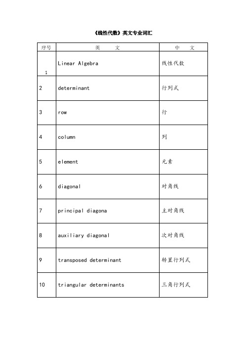
44
an adjoint matrix
伴随矩阵
45
singular matrix
奇异矩阵
46
nonsingular matrix
非奇异矩阵
47
elementary transformations
初等变换
48
vectors
向量
49
components
分量
50
linearly combination
矩阵m×n
38
the determinant of matrix A
方阵A的行列式
39
operations on Matrices
矩阵的运算
40
a transposed matrix
转置矩阵
41
an inverse matrix
逆矩阵
42
an conjugate matrix
共轭矩阵
43
an diagonal matrix
范德蒙行列式
24
bordered determinant
加边行列式
25
reduction of the order of a determinant
降阶法
26
method of Recursion relation
递推法
27
induction
归纳法
28
Cramer´srule
克莱姆法则
29
matrix
98
canonical form
标准型
99
the canonical form of a quadratic form
二次型的标准型
100
- 1、下载文档前请自行甄别文档内容的完整性,平台不提供额外的编辑、内容补充、找答案等附加服务。
- 2、"仅部分预览"的文档,不可在线预览部分如存在完整性等问题,可反馈申请退款(可完整预览的文档不适用该条件!)。
- 3、如文档侵犯您的权益,请联系客服反馈,我们会尽快为您处理(人工客服工作时间:9:00-18:30)。
exp{−|x |} F (w(x )),
(5)
which we shall call a skew-symmetric-Laplace distribution. The Laplace distribution has been commonly used as an alternative to the normal distribution. It has also attracted interesting applications in modeling. The main feature of the family of skewsymmetric-Laplace distributions in (5) is that some new parameters are introduced to control skewness and kurtosis and provide a more flexible model which represents the data as adequately as possible. Thus, we can expect this to be useful in more practical situations. In Sect. 2, we shall study some properties of this new family and also consider its truncated situation in general. In Sect. 3, some of its related
Keywords Skew-normal distribution · Skew-symmetric distribution · Stochastic ordering
1 Introduction
Recently, much of interest has been shown on a family of distributions called “SkewSymmetric” with probabilitБайду номын сангаас density function (pdf)
Stat Papers (2012) 53:685–696 DOI 10.1007/s00362-011-0372-7 REGULAR ARTICLE
A family of skew-symmetric-Laplace distributions
V. Nekoukhou · M. H. Alamatsaz
2 f (x)F(λx),
(4)
which is called a skew-Laplace distribution. In particular, Aryal and Rao (2005) studied some properties of truncated skew-Laplace distribution and Kozubowski and Nolan (2008) showed that a skew-Laplace distribution is infinitely divisible.
123
A family of skew-symmetric-Laplace distributions
687
stochastic orderings are discussed. Because of importance of normal distribution in statistical literature, a special member of this general family which we call generalized skew-symmetric-Laplace-normal distribution, will be discussed in Sect. 4, where more properties of this distribution will be revealed.
Definition 1 A random variable X is distributed as a skew-symmetric-Laplace distribution, denoted by SS L(F, w), if its density function has the form
(i) 0 ≤ κ(x) ≤ 1, x ∈ R, (ii) κ(x) + κ(−x) = 1, a.e. on R.
Particularly, κ can be an absolutely continuous symmetric distribution function. As a special case, κ can be the cumulative distribution function (cdf) of f ; see, e.g., Arnold and Lin (2004).
2 The family of skew-symmetric-Laplace distributions
Gómez et al. (2007) presented a generalized family of skew-symmetric distributions in the form
2 f (x)F(w(x)),
where f is a symmetric pdf and investigated only the case where F is the cdf of a standard normal distribution and w is an odd continuous function. Here, we shall fix f as pdf of a Laplace distribution but F is taken arbitrary.
2φ(x) (λx)
(3)
in which φ and are the standard normal density and distribution functions, respectively. Another known case is when f and F are the density and distribution functions of Laplace distribution, respectively:
V. Nekoukhou e-mail: v.nekoukhou@
123
686
V. Nekoukhou, M. H. Alamatsaz
where f is a symmetric pdf (about zero) and κ is a lebesgue measurable function satisfying
2 f (x)κ(x),
(1)
V. Nekoukhou · M. H. Alamatsaz (B)
Department of Statistics, University of Isfahan, Isfahan, Iran e-mail: alamatho@sci.ui.ac.ir; mh−alamatsaz@
In this paper, a more general family of skew-Laplace distributions is introduced which contains the skew-Laplace distribution (4) as a special case. Here, we consider F as an arbitrary symmetric cdf and replace λx by any odd continuous function w. That is,
Recall that X is distributed as Laplace distribution with location parameter μ and scale parameter σ if its pdf is
f (x)
=
1 2σ
exp
− |x
− σ
μ|
,
x ∈ R,
(6)
denoted by X ∼ L(μ, σ ). For simplicity, we consider the case that μ = 0 and σ = 1, i.e., the standard Laplace distribution.
Received: 13 September 2009 / Revised: 11 December 2010 / Published online: 22 February 2011 © Springer-Verlag 2011
Abstract Skew-symmetric distributions of various types have been the center of attraction by many researchers in the literature. In this article, we shall introduce another more general class of skew distributions, specially related to the Laplace distribution. This new class contains some previously known skew distributions. We shall investigate different characteristics of members of this class such as its moments, thus generalizing a result of Umbach (Stat Probab Lett 76:507–512, 2006), limiting behavior, moment generating function, unimodality and reveal its natural occurrence as the distribution of some order statistics. In addition, we will generalize a result of Aryal and Rao (Nonlinear Anal 63:639–646, 2005) in connection with truncated skew-Laplace distribution and study its certain stochastic orderings. Some illustrative examples are also provided.