Robust frequency
FSK信号调制与解调技术
1 引言1.1 研究的背景与意义现代社会中人们对于通信设备的使用要求越来越高,随着无线通信技术的不断发展,人们所要处理的各种信息量呈爆炸式地增长。
传统的通信信号处理是基于冯·诺依曼计算机的串行处理方式,利用传统的冯·诺依曼式计算机来进行海量信息处理的话,以现有的技术,是不可能在短时间内完成的。
而具于并行结构的信息处理方式为提高信息的处理速度提供了一个新的解决思路。
随着人们对于通信的要求不断提高,应用领域的不断拓展,通信带宽显得越来越紧张。
人们想了很多方法,来使有限的带宽能尽可能的携带更多的信息。
但这样做会出现一个问题,即:信号调制阶数的增加可以提升传送时所携带的信息量,但在解调时其误码率也相应显著地提高。
信息量不断增加的结果可能是,解调器很难去解调出本身所传递的信息.如果在提高信息携带量的同时,能够找到一种合适的解调方式,将解调的误码率控制在允许的范围内,同时又不需要恢复原始载波信号,从而降低解调系统的复杂程度,那将是很好的。
通信技术在不断地发展,在现今的无线、有线信道中,有很多信号在同时进行着传递,相互之间都会有干扰,而强干扰信号也可能来自于其它媒介。
在军事领域,抗干扰技术的研究就更为必要。
我们需要通信设备在强干扰地环境下进行正常的通信工作.目前常用的通信调制方法有很多种,如FSK、QPSK、QAM等。
在实际的通信工程中,不同的调制制式由于自身的特点而应用于不同场合,而通信中不同的调制、解调制式就构成了不同的系统.如果按照常规的方法,每产生一种信号就需要一个硬件电路,甚至一个模块,那么要使一部发射机产生几种、几十种不同制式的通信信号,其电路就会异常复杂,体积重量都会很大。
而在接收机部分,情况也同样是如此,即对某种特定的调制信号,必须有一个特定的对应模块电路来对该信号进行解调工作。
如果发射端所发射的信号调制方式发生改变,这一解调模块就无能为力了。
实际上,随着通信技术的进步和发展,现代社会对于通信技术的要求越来越高,比如要求通信系统具有最低的成本、最高的效率,以及跨平台工作的特性,如PDA、电脑、手机使用时所要求的通用性、互连性等。
利用训练序列的OFDM系统定时同步算法RobustTimingSynchronization..
利用训练序列的OFDM系统定时同步算法胡畅华杨明武合肥工业大学电子科学与应用物理学院,合肥230009摘要:在OFDM系统中,定时同步的好坏严重影响到接收端的接收。
通过对各种已有定时同步方法的分析,利用CAZAC序列的良好特性,提出一种基于CAZAC训练序列的定时同步方法。
改进后的算法能够很好地改善原有经典算法的峰值平台及测量不精确的问题。
通过高斯白噪声信道仿真,证明了改进算法在定时同步方面较经典算法有明显提高。
正交频分复用;定时估计;CAZAC序列;同步算法TN92 A1004-3365(2011)05-0722-03Robust Timing Synchronization Algorithm for OFDM System Using Training Sequence HU ChanghuaYANG Mingwu2011-01-172011-02-193 定时同步检测算法@@[1] 佟学俭,罗涛.OFDM移动通信技术原理与应用 [M].北京:人民邮电出版社,2003:83-116.@@[2]尹长川,罗涛,乐新光.多载波宽带无线通信技术 [M].北京:北京邮电大学出版社,2004:13-19,42-70.@@[3] CHU D C. Polyphase codes with good periodic corre lation properties [J]. IEEE Trans Inform Theo,1972, 18(4): 531-532.@@[4] POPOVIC B M. Generalized chirp-like polyphase se quences with optimum correlation properties [J]. IEEE Trans Infor Theo, 1992, 38(4) : 1406-1409.@@[5] FRANK R L, ZADOFF S A. Phase shift pulse codes with good periodic correlation properties [J]. IEEE Trans Inform Theory, 1962, 8(6): 381-382.@@[6] LI L, ZHOU P. Synchronization for B3G MIMO OFDM in DL_ initial acquisition by CAZAC sequence [C] // IEEE Int Conf Commtn Circ Syst Proc. Gui lin, China. 2006, 2: 1035-1039.@@[7] SCHMIDL T M, COX D C. Robust frequency and timing synchronization for OFDM [J]. IEEE Trans Commun, 1997, 45(12): 1613-1621.@@[8] MINN H, ZENG M, BHARGAVA V K. On timing offset estimation for OFDM system [J]. IEEE Com mun Lett, 2000, 4(7): 242-244. 胡畅华(1986-),女(汉族),重庆人,硕士研究生,研究方向为集成电路设计与工艺技术。
Efficient frequency-domain realization of robust generalized, sidelobe cancellers
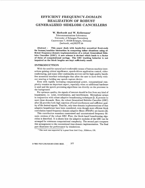
Figure 1: Conventional robust time-domain GSC after [A']
xed Beamforming
The FBF which is usually a delay&sum beamformer enhances desired signal components, and is used as reference for the adaptation of the adaptive sidelobe cancelling path. The fractional time-delays that are required in the discretized time domain for the steering into the assumed target direction-of-arrival (DOA) are usually realized by short fractional delay filters. Consequently, both modules, FBF ancl beamsteering are realized more efficiently in the time domain than in the frequency domain. Then, the combination with the ABM is computationally more efficient. The FBF thus simply sums up the steered sensor signals z,,(n), or: yj(n) = Pd- 1 C7R=0 n is the discrete time variable, M is the number of microz,,(n). phones.
基于信号频谱特性的配电网故障行波检测方法

第52卷第9期电力系统保护与控制Vol.52 No.9 2024年5月1日Power System Protection and Control May 1, 2024 DOI: 10.19783/ki.pspc.231451基于信号频谱特性的配电网故障行波检测方法刘 丰1,谢李为1,蔡 军2,喻 锟1,王有鹏1,曾祥君1,唐 欣1(1.长沙理工大学电气与信息工程学院,湖南 长沙 410114;2.国网湖南省电力有限公司长沙供电分公司,湖南 长沙 410015)摘要:针对配电网干扰情况下微弱故障信号特征不明显导致行波采集设备难以有效检测故障行波信号的问题,提出一种基于信号频谱特性的配电网故障行波检测方法。
首先,通过分析配电网故障行波的传输特征与频率特性,建立基于波形增量比值的启动判据,对设备采样数据进行预处理,减少行波定位装置的误启动。
然后,引入鲁棒性局部均值分解(robust local mean decomposition, RLMD)方法处理采样数据,滤除采样过程中的干扰信号,减少噪声信号的影响。
最后,根据行波低频含量衰减较小而高频含量衰减快的性质,建立故障行波辨识判据,辨识配电网故障行波信号。
仿真表明,所提方法能够有效检测微弱故障时的行波信号。
关键词:配电网;故障行波检测;RLMD;多分支线路A fault traveling wave detection method based on signal spectral characteristicsfor a distribution networkLIU Feng1, XIE Liwei1, CAI Jun2, YU Kun1, WANG Youpeng1, ZENG Xiangjun1, TANG Xin1(1. School of Electrical & Information Engineering, Changsha University of Science & Technology, Changsha 410114, China;2. Changsha Power Supply Branch, State Grid Hunan Electric Power Co., Ltd., Changsha 410015, China)Abstract: There is a problem in that the characteristics of weak fault signals are not obvious when there is interference on the distribution network. This makes it difficult for traveling wave acquisition equipment to effectively detect the fault traveling wave signals. Thus a method of fault traveling wave detection based on signal spectral characteristics is proposed. By analyzing the transmission characteristics and frequency characteristics of the fault traveling wave in distribution networks, a start-up criterion is established based on the waveform incremental ratio. It can preprocess the sampling data of the equipment, and reduce the false start-up of the traveling wave equipment. Then, the robust local mean decomposition (RLMD) method is used to process the sampling data, filter out the interference signal during the sampling process, and reduce the influence of the noise signal. Finally, given that it is a characteristic of the traveling wave that the low-frequency content attenuates less but the high-frequency content attenuates faster, an identification criterion is established to identify the fault traveling wave signals. Simulations show that the proposed method can effectively detect the fault traveling wave signals during weak faults.This work is supported by the National Natural Science Foundation of China (No. U22B20113).Key words: distribution network; fault traveling wave detection; RLMD; multi-branches0 引言配电网线路分布广泛且运行环境复杂[1-3]。
Robust Control

Robust ControlRobust control is a field of engineering and mathematics that deals with the design and implementation of control systems that can effectively handle uncertainty and variations in the system being controlled. This is an important area of study because in real-world applications, systems are often subject to various disturbances and uncertainties that can affect their behavior. Robust control aims to ensure that the system remains stable and performs as desired despite these uncertainties. One perspective on robust control is from the standpoint of aerospace engineering. In the field of aerospace, robust control is crucial for ensuring the stability and performance of aircraft and spacecraft. These vehicles operate in highly uncertain and dynamic environments, and their control systems must be able to adapt to changing conditions while maintaining stability and safety. Robust control techniques such as H-infinity control and mu-synthesis have been widely used in aerospace applications to design control systems that can handle uncertainties in the aerodynamic properties of the vehicle, variations in the operating conditions, and disturbances such as gusts and turbulence. Another perspective on robust control comes from the field of robotics. In robotics, control systems must be able to handle uncertainties in the dynamics of the robot and variations in the environment in which it operates. Robust control techniques such as sliding mode control and adaptive control have been applied to develop robot control systems that can maintain stability and achieve desired performance in the presence of uncertainties. This is particularly important for applications such as autonomous vehicles, where the robot must be able to operate in diverse and changing environments. From a theoretical perspective, robust control is grounded in the field of control theory and optimization. The development of robust control techniques involves the use of mathematical tools such as linear matrix inequalities (LMIs), convex optimization, and frequency domain analysis. These tools are used to formulate and solve the robust control design problem, which involves finding a control law that ensures stability and performance for a given range of uncertainties. The theoretical aspects of robust control are often complex and require a deep understanding of mathematical concepts, making it a challenging but intellectually rewarding fieldof study. In the industrial automation and process control domain, robust control plays a critical role in ensuring the stability and performance of industrial processes. Many industrial processes are subject to uncertainties and disturbances, such as variations in the parameters of the process, external disturbances, and equipment faults. Robust control techniques such as model predictive control (MPC) and robust PID control have been applied to address these challenges and improve the performance of industrial processes. Robust control is essential for maintaining the safety, efficiency, and quality of industrial operations, makingit an integral part of modern industrial automation systems. One of the key challenges in robust control is the trade-off between performance and robustness. In many cases, increasing the robustness of a control system may come at the cost of reduced performance, and vice versa. For example, a control system that is designed to be highly robust to uncertainties may exhibit conservative behaviorand may not be able to achieve the desired level of performance. On the other hand, a control system that is optimized for performance may be sensitive touncertainties and disturbances, leading to instability or poor performance in the presence of such disturbances. Balancing the trade-off between performance and robustness is a fundamental challenge in robust control design, and it requires careful consideration of the specific requirements and constraints of the application. In conclusion, robust control is a critical area of study in engineering and mathematics, with applications in aerospace, robotics, industrial automation, and many other fields. It addresses the challenge of designing control systems that can handle uncertainties and variations in the system being controlled, ensuring stability and performance in the presence of disturbances. Robust control techniques have been developed and applied in diverse domains, and they continue to be an active area of research and development. The theoreticaland practical aspects of robust control present both challenges and opportunities for engineers and researchers, making it a fascinating and important field of study.。
robustperiod算法复现
robustperiod算法复现下面是使用Python实现robustperiod算法的示例代码:pythonimport numpy as npdef robustperiod(signal, min_period=10, max_period=None): """Robust Period Estimation AlgorithmArgs:signal: 输入信号min_period: 最小周期长度max_period: 最大周期长度Returns:period: 估计的信号周期"""N = len(signal)max_lags = N 2if max_period is None:max_period = Nassert min_period <= max_period, "最小周期长度应小于等于最大周期长度"max_ac = float('-inf')opt_lag = 0for lag in range(min_period, max_period+1):auto_correlation = np.correlate(signal, np.roll(signal, lag)) / Nac = auto_correlation[0]if ac > max_ac:max_ac = acopt_lag = lagperiod = opt_lagreturn period该算法的基本思想是计算输入信号的自相关函数,找到在给定范围内具有最大自相关值的滞后时间,然后将该滞后时间作为信号的周期。
其中,`np.correlate()`函数用于计算信号的互相关(cross-correlation),`np.roll()`函数用于实现滞后操作。
示例运行代码:pythonsignal = [1, 2, 3, 4, 5, 4, 3, 2, 1]period = robustperiod(signal)print("Estimated period:", period)输出结果为:Estimated period: 8这表示输入信号的周期估计为8。
FREQUENCYCONTROL
Effects of frequency on motor load
• Motor load
• An approximate rule of thumb is that the connected motor load magnitude decreases by 2% if the frequency decreases by 1%.
• REG DOWN RESERVE
• Generation resources that decrease generation • Controllable load resources that increase load
• Responsive Reserve (RRS)
• Arrest frequency decay within the first few seconds of a significant frequency deviation on the ERCOT Transmission Grid using Primary Frequency Response and interruptible Load;
• Non Motor load
• It is a reasonably accurate statement to say that non-motor load magnitude does not vary as frequency is varied.
•Composite Load/Frequency Effect
Frequency control
ERCOT SCADA AGC
Load Frequency control
SecurityConstrained Economic Dispatch (SCED)
robust tests for equality of variances解读

robust tests for equality of variances解读"Robust tests for equality of variances" 的中文翻译是“方差的稳健性检验”。
这里,我们逐一解释这些术语:Robust tests(稳健性检验):在统计学中,一个“稳健”的测试是指即使在违反了某些假设的情况下,该测试仍然能够保持其有效性或至少不会受到太大的影响。
换句话说,当数据不满足某些理想条件时,稳健性检验仍然可以给出可靠的结果。
Equality of variances(方差齐性):这是指两组或多组数据的方差是否相等。
在某些统计测试中,例如t检验或方差分析(ANOVA),一个基本假设是不同组的方差应该是相等的。
如果不满足这个假设,那么这些测试的结果可能是不准确的。
因此,“Robust tests for equality of variances”是指那些用于检查两组或多组数据的方差是否相等的测试,并且这些测试在数据不满足某些理想条件时仍然是可靠的。
常见的方差齐性检验包括:Levene's Test:它基于每个数据点与其组内均值的绝对偏差。
Levene's Test 比传统的F-test 更稳健,因为它不假设数据来自正态分布。
Bartlett's Test:这是基于卡方分布的检验,用于检验k个样本是否来自方差相等的总体。
Fligner-Killeen Test:这是另一种非参数的方差齐性检验方法,适用于非正态分布的数据。
当数据不符合正态分布或其他假设时,使用这些稳健性检验可以为我们提供更大的信心来确定方差的差异是否显著。
除了上述提到的方差齐性检验方法,还有一些其他的方法也可以用于检验方差的稳健性。
例如:Brown-Forsythe Test:它是基于中位数和绝对偏差的方差齐性检验方法,适用于非正态分布数据。
与Levene's Test类似,它也是一种比传统的F-test更稳健的方法。
- 1、下载文档前请自行甄别文档内容的完整性,平台不提供额外的编辑、内容补充、找答案等附加服务。
- 2、"仅部分预览"的文档,不可在线预览部分如存在完整性等问题,可反馈申请退款(可完整预览的文档不适用该条件!)。
- 3、如文档侵犯您的权益,请联系客服反馈,我们会尽快为您处理(人工客服工作时间:9:00-18:30)。
Robust Frequency and Timing Synchronization for OFDMTimothy M.Schmidl and Donald C.Cox,Fellow,IEEEAbstract—A rapid synchronization method is presented for an orthogonal frequency-division multiplexing(OFDM)system using either a continuous transmission or a burst operation over a frequency-selective channel.The presence of a signal can be detected upon the receipt of just one training sequence of two symbols.The start of the frame and the beginning of the symbol can be found,and carrier frequency offsets of many subchannels spacings can be corrected.The algorithms operate near the Cram´e r–Rao lower bound for the variance of the frequency offset estimate,and the inherent averaging over many subcarriers allows acquisition at very low signal-to-noise ratios(SNR’s). Index Terms—Carrier frequency,orthogonal frequency-division multiplexing,symbol timing estimation.I.I NTRODUCTIONI N AN orthogonal frequency-division multiplexing(OFDM)system,synchronization at the receiver is one important step that must be performed.This paper describes a method to acquire synchronization for either a continuous stream of data as in a broadcast application or for bursty data as in a wireless local area network(WLAN).In both cases the receiver must continuously scan for incoming data,and rapid acquisition is needed.The ratio of the number of overhead bits for synchronization to the number of message bits must be kept to a minimum,and low-complexity algorithms are needed. Synchronization of an OFDM signal requiresfinding the symbol timing and carrier frequency offset.Symbol timing for an OFDM signal is significantly different than for a single carrier signal since there is not an“eye opening”where a best sampling time can be found.Rather there are hundreds or thousands of samples per OFDM symbol since the number of samples necessary is proportional to the number of subcarriers. Finding the symbol timing for OFDM meansfinding an estimate of where the symbol starts.There is usually some tolerance for symbol timing errors when a cyclic prefix is used to extend the symbol.Synchronization of the carrier frequency at the receiver must be performed very accurately, or there will be loss of orthogonality between the subsymbols. OFDM systems are very sensitive to carrier frequency offsets since they can only tolerate offsets which are a fraction of the Paper approved by M.Luise,the Editor for Synchronization of the IEEE Communications Society.Manuscript received April16,1996;revised February11,1997.This work was supported in part by a National Science Foundation Graduate Fellowship.This work was presented in part at the IEEE International Conference on Communications(ICC),Dallas,TX,June1996. T.M.Schmidl is with DSP Research and Development Center at Texas Instruments Incorporated,Dallas,TX75243USA(e-mail:schmidl@).D. C.Cox is with the STAR Laboratory,Department of Electrical Engineering,Stanford University,Stanford,CA94305-4055USA(e-mail: dcox@).Publisher Item Identifier S0090-6778(97)09083-1.spacing between the subcarriers without a large degradation in system performance[1].There have been several papers on the subject of synchro-nization for OFDM in recent years.Moose gives the maximum likelihood estimator for the carrier frequency offset which is calculated in the frequency domain after taking the FFT[2]. He assumes that the symbol timing is known,so he just has to find the carrier frequency offset.The limit of the acquisition range for the carrier frequency offsetisFig.1.Block diagram of OFDM transmitter.Fig.2.Block diagram of OFDM receiver.of carrier frequency offset.The method in this paper avoidsthe extra overhead of using a null symbol,while allowinga large acquisition range for the carrier frequency offset.Byusing one unique symbol which has a repetition within half asymbol period,this method can be used for bursts of data tofind whether a burst is present and tofind the start of the burst.Acquisition is achieved in two separate steps through theuse of a two-symbol training sequence,which will usuallybe placed at the start of the frame.First the symbol/frametiming is found by searching for a symbol in which thefirst half is identical to the second half in the time domain.Then the carrier frequency offset is partially corrected,anda correlation with a second symbol is performed tofindthe carrier frequency offset.II.OFDM P RINCIPLESThe OFDM signal is generated at baseband by taking theinverse fast Fourier transform(IFFT)of quadrature amplitudemodulated(QAM)or phase-shift keyed(PSK)subsymbols(Fig.1).In thefigure,the block P/S representsa parallel-to-serial converter.An OFDM symbol has a usefulperiodsubcarriers is given by(2)SCHMIDL AND COX:ROBUST FREQUENCY AND TIMING SYNCHRONIZATION FOR OFDM 1615TABLE I I LLUSTRATIONOFU SEOFPN S EQUENCESFORT RAINING SYMBOLSand the IF local oscillator for the quadrature branch at the receiveras.Thedemodulated signal before the sampler can be expressedasmeans to low-pass filter the terms in theargument.The output of the in-phase branch is considered to be real and the output of the quadrature branch is considered to be imaginary.This is a mathematical convention to represent the in-phase and quadrature components as a complex number.After sampling,the complex samples are denotedas.Consider the first training symbol where the first half is identical to the second half (in time order),except for a phase shift caused by the carrier frequency offset.If the conjugate of a sample from the first half is multiplied by the correspondingsample from the second half(seconds later),the effect of the channel should cancel,and the result will have a phase ofapproximatelycomplex samples in one-half of the firsttraining symbol (excluding the cyclic prefix),and let the sum of the pairs of productsbe(5)which can be implemented with the iterativeformulais a time index corresponding to the first sample ina windowofsamples.This window slides along in time as the receiver searches for the first training symbol.The received energy for the second half-symbol is definedby(7)Fig.3.Example of the timing metric for the AWGN channel (SNR =10dB).which can also be calculatediteratively.(8)Fig.3shows an example of the timing metric as a window slides past coincidence for the AWGN channel for an OFDM signal with 1000subcarriers,a carrier frequency offset of 12.4subcarrier spacings,and an signal-to-noise ratio (SNR)of 10dB,where the SNR is the total signal (all the subcarriers)to noise power ratio.The timing metric reaches a plateau which has a length equal to the length of the guard interval minus the length of the channel impulse response since there is no ISI within this plateau to distort the signal.For the AWGN channel,there is a window with a length of the guard interval where the metric reaches a maximum,and the start of the frame can be taken to be anywhere within this window without a loss in the received SNR.For the frequency selective channels,the length of the impulse response of the channel is shorter than the guard interval by design choice of the guard interval,so the plateau in the maximum of the timing metric is shorter than for the AWGN channel.This plateau leads to some uncertainty as to the start of the frame.For the simulations in this paper,OFDM symbols are generated with 1000frequencies,1616IEEE TRANSACTIONS ON COMMUNICATIONS,VOL.45,NO.12,DECEMBER1997 set for this detection.Second,there is some degradation inperformance if the symbol timing estimate deviates from thecorrect region.Simulations are performed tofind the effect ofextra interference that is introduced by poor symbol timingestimates for two types of channels.1)Distribution of Timing Metric:Let each complex sam-ple be made up of a signal and a noisecomponent.Let the variance of the real and imaginary com-ponentsbe:(9)(10)so that the SNRis.This is just another way of looking atthe problem with a new set of axes with one axis inthe(12)where means the component intheand add in-phase,while all the other termsadd with random phases.By the central limit theorem(CLT),terms,the magnitude of each term could be taken byadding the squares of the real and imaginary parts.Instead,we can define a new set of orthogonal axes in which one axisis in the direction of thetermmeans to take the component inthe directionof.Note that for usable values ofSNR,the mean is much greater than the standard deviation.Thus,for the Gaussian approximation,the probabilityofby a Gaussian reasonable.Anotherequivalent way of thinking about the distribution isthatis Rician with the mean much larger than the standarddeviation.In this case the Gaussian approximation may beused[8].Define the square rootofis Gaussianwith(15)This can be justified because linear operations on a Gauss-ian random variable will result in another Gaussian randomvariable[9].When calculating the variance,notethat(16)andSCHMIDL AND COX:ROBUST FREQUENCY AND TIMING SYNCHRONIZATION FOR OFDM1617 Since these terms are the same in both the numerator anddenominator,they do not contribute to the overall variance.Then(17)is(18)where is used to denote a Gaussian random variablewith a meanof.The valueof also can give an estimate of the SNR,whichisis so close to1that an accurate estimate ofthe SNR can not be determined,but only that the SNR is high.For example,if,then dB.This can be used to set a threshold so that very weak signalswill not be decoded,or it can be used in a WLAN to feed backto the transmitter to indicate what data rate will be supportedso that an appropriate constellation and code can be chosen.Alookup table can be implemented basedon,so thatno square roots or divisions need to be performed.Even if there is a frequency selective channel,all the signalenergy will go into the signal component term except whenthe length of the channel impulse response becomes so largethat it is longer than the cyclic prefix.At this point,the energylocated at longer delays becomes interference and would beadded to the noise terms.At a position outside thefirst training symbol,the terms inthesum add with random phases since there is nota periodicity for samples spacedbyare Gaussian by the CLT.The sum ofthe square of two zero-mean Gaussian random variables,eachwith a variance of1is a chi-square random variable withtwo degrees of freedom and is represented by thesymbol.The meanof is2and the variance is4[9].To simplifythe computations,let the variance of the real and imaginarycomponentsofbe:arehas a Gaussian distribution bythe CLT,and its square is also Gaussian because the standarddeviation is much smaller than the mean.Again,this is alinear operation on a Gaussian random variable(using theapproximation),so the result is also Gaussian.Thus,(27)wherethe(28)Here,the variance of the Gaussian random variable is propor-tionalto1618IEEE TRANSACTIONS ON COMMUNICATIONS,VOL.45,NO.12,DECEMBER1997Fig.4.Expected value of timing metric with L =512.Dashed lines indicate three standarddeviations.Fig.5.Mean and variance at the correct timing point with L =512for the exponential channel.of the timing metricare(29)and ,while the calculation assumes that they areindependent.2)Probability of Missing the Training Sequence or of False Detection:The probability distributions calculated inSectionFig.6.Mean and variance at an incorrect timing point with L =512for the exponential channel.III-B-1can be used to determine both the probability of not detecting a training sequence when one is present and of falsely detecting a training sequence when one is not present.As an example of how this can be done,let there be 1000subchannels andlet .If the system is designed to detect a signal if the SNR is at least 10dB,then from Eqs.(19)and (20),when the signal is present the mean is 0.827and the varianceis ,so the standard deviationisat the correct timing.If no signal is present,thenfrom (28)the meanis and the standard deviation isalso .If the threshold is set at 0.1,then the margin for error when the training signal is presentis,this requires that the threshold be 3.1standard deviations below the mean found with (19).When computing the probability of false detection,note that the training signal is not present for most of each frame.If there are 100OFDM symbols within one frame,then most of the time the training symbol is not present.Since the sliding windows for the symbol timing estimator are half a symbol long,there can be about 200uncorrelated values of the symbol timing estimator within one frame.If the probability of false detection within one frame is desired tobe ,then the probability of false detection at any point in time should beabout .From [10]the cumulative distribution functionforisrequiresto be less than 24.4,which correspondstostandard deviations.(34)SCHMIDL AND COX:ROBUST FREQUENCY AND TIMING SYNCHRONIZATION FOR OFDM1619Fig.7.Relationship of signal,noise,and interference power to the symbol timing position for the AWGN channel.The shaded portion in thefirst plot indicates the range where the synchronizer can estimate the start of the symbol to maximize SNIR.In this example,both the probabilities of missing a trainingsequence or of false detection within one frame are lessthan.This allows the threshold to be adjusted to operate at a lower SNR if that is desired.Another option is to reduce the amount of computation performed while searching for the training sequence by not processing every sample.This could be useful in a burst mode when data may not arrive very often.3)Reduction in SNIR:Two channels are used in simula-tions to measure the performance of the estimation algorithms. First the AWGN channel is used to show how the algorithms perform on a benign channel,and it is also used as a basis for comparison.Then a frequency selective channel with an exponential power delay profile is used to show that the algorithms perform well in a more realistic environment. Sixteen paths are chosen with path delays of0,4,8,th pathand is the delayof thetois the variance of the intersymbol interference(ISI)added by incorrect symbol timing.Fig.7plots the averagesignal,noise,and interference power levels versus time for anAWGN channel.Note that interference here refers to the ISIfrom symbols before and after the training symbol in the timedomain.The timefrom is the length of the guardinterval,and the timefrom is the length of the usefulpart of the OFDM symbol.If the synchronizer estimates thatthe useful part of the symbol starts at any time within the guardinterval,which is the shaded area in thefirst plot of Fig.7,then there is no reduction in SNIR due to incorrect symboltiming.However,if the synchronizer estimates that the startTABLE IIR EDUCTION IN SNIR(dB)D UE TO E RRORS IN S YMBOL TIMINGof the symbol is outside the guard interval,there will be botha decrease in signal energy and an increase in interference,resulting in a lower SNIR.This occurs because samples fromthe previous or next symbol are input into the FFT along withsamples from the current symbol.For example,if the start ofthe symbol is estimated to be at eithertimeis reduced by the length ofthe channel impulse response.Two methods to determine the symbol timing are comparedon the basis of reduction in SNIR.Thefirst method is tosimplyfind the maximum of the timing metric.The secondmethod is tofind the maximum,find the points to the left andright in the time domain,which are90%of the maximum,and average these two90%times tofind the symbol timingestimate.The rationale behind this method is that the besttiming points typically lie in a plateau.By trying to determinethe center of this plateau,it is more likely that the estimatewill not fall slightly off the plateau.Table II compares the twomethods on the basis of reduction in SNIR for the AWGN andfrequency selective channel.For each type of channel,10000simulations are run at each SNR,and in each run,different PNsequences,channels,and noise are generated.The averagingmethod performs significantly better than simplyfinding thepeak of the timing metric,and it involves only slightly morecomputation.With a40-dB SNR,a symbol timing offset of onesample away from the plateau would result in about10dB indegradation in SNIR for the AWGN channel.The averagingmethod offinding the symbol time resulted in no degradationin10000runs for the AWGN channel and a degradation of justunder0.06dB for the exponential channel at an SNR of40dB.IV.E STIMATION OF C ARRIER F REQUENCY O FFSETA.Carrier Frequency Offset Estimation AlgorithmThe main difference between the two halves of thefirsttraining symbol will be a phase differenceof(38)1620IEEE TRANSACTIONS ON COMMUNICATIONS,VOL.45,NO.12,DECEMBER 1997near the best timing point.If,then the frequency offset estimateisis an integer.By partially correcting the frequencyoffset,adjacent carrier interference (ACI)can be avoided,and then the remaining offsetofis unknown,this additional phase shift is unknown.However,since the phase shift is the same for each pair of frequencies,a metric similar to (8)can be used.Letspanning the range of possible frequency offsetsand(43)Since the carrier frequency offset estimate (in subcarrier spacings)is made up of the sum of the initial estimate and an even integer,the variance of the initialestimate,(44)This is not surprising because Moose shows that his estimator is the maximum-likelihood estimator (MLE)of differential phase,and Rife states that the Cram´e r–Rao bounds are almost met by the MLE with high SNR.Since the frequency offset estimate is made by averaging over hundreds or thousands of subcarriers,the effective SNR is usually very high.To illustrate that the frequency acquisition range is greatly widened with this new method,Fig.8compares the error variance for Moose’s frequency estimation methods (with two repeated half-symbols)with the new method for 1000carriers with an SNR of 10dB.The simulations were performed with 10000runs per frequency offset value.Since Moose’s method is designed to work only with a very small frequency offset,it fails for larger frequency offsets.In Fig.8,the Cram´e r–Rao boundis .Note that the simulation here for Moose’s algorithm uses the shortened symbols as described in [2],which results is a frequency acquisition rangeofSCHMIDL AND COX:ROBUST FREQUENCY AND TIMING SYNCHRONIZATION FOR OFDM1621parison of carrier frequency offset estimate to Cram´e r–Raobound.Fig.10.Expected value of carrier frequency offset metric with W=500.Dashed lines indicate three standard deviations.At high SNR the mean is approximately1,and the varianceis approximately.At an incorrect frequency offset the signal products nolonger add in phase,and has a chi-square dis-tribution with two degrees of freedom with(47)(48)Fig.10shows a plot of the expected value of frequencyoffset metric。