财管专业——《管理会计(双语)》

合集下载

《管理会计》课件全英文Acct_ch1_ManAcct_(Feb_25)

1. Externally focused 2. Must follow externally imposed rules 3. Objective financial information
1 -23
Types of Information
For management accounting, the The restrictions imposed on financial accounting tend to financial or nonfinancial produce objectivebe much more information may and verifiable financial information. subjective in nature.
Continued
1 -3
Objectives
5. Describe the role of management accountants in an organization. 6. Explain the importance of ethical behavior for managers and management accountants. 7. List three forms of certification available to management accountants.
1 -12
Management Process
The Management Process is defined by the following activities: Planning Controlling Decision Making
Decision making is the process of choosing among competing alternatives.

管理会计双语第5章

Sales level at which operating income is zero Sales above breakeven result in a profit Sales below breakeven result in a loss Two methods: Income statement approach Contribution margin approach
Units produced Direct materials cost per unit Total direct materials cost
100 200 300
$120 $60 $40
12,000 12,000 12,000
400
500
$30
$24
12,000
12,000
Committed fixed costs represent investments with a
Contribution margin is used first to cover fixed expenses.
Any remaining contribution margin contributes to net operating income.
Sales revenue per unit
Fixed costs Contribution margin ratio
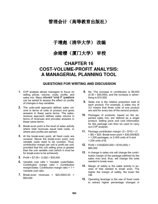
Breakeven point in sales dollars
$20,000 $15,000
Dollars
$10,000 $5,000 $0 0 500
•
Revenues
1,000
1,500
Volume of Units

大学会计类专业阅读书籍推荐

大学会计类专业的学生推荐的阅读书籍•《会计原理》（Accounting Principles）：作者是美国著名的会计学家韦伯，是会计领域的经典教材之一。

该书系统地阐述了会计的基本概念、原则和方法，适合作为入门读物。

•《会计基础》（Financial Accounting）：作者是美国著名的会计学家韦尔斯，这本书被广泛用于大学本科的会计课程。

它详细介绍了财务会计的基本概念、原则和实务操作，对于理解财务报表的编制和分析非常有帮助。

•《管理会计》（Management Accounting）：作者是美国著名的管理会计学家安东尼，本书对管理会计的概念、原则、方法、技巧等方面进行了全面深入的探讨。

它有助于理解企业在管理决策中如何运用会计信息。

•《会计研究方法》（Research Methods in Accounting）：同样是安东尼所著，这本书详细介绍了会计研究的各种方法和技巧，对于进行会计研究或撰写相关论文的学生非常有用。

•《成本会计学》：作者是中国著名的成本会计学专家李冠英教授，本书介绍了成本会计的基本概念、原则、方法和技巧，涵盖了成本核算、成本控制、成本分析等方面的内容。

对于理解企业的成本管理和决策非常有帮助。

此外，还有以下一些值得一读的会计类书籍：•《公司理财》（Corporate Finance）：作者是斯蒂芬A.罗斯等人，这本书是财务管理学的权威著作，涵盖了公司理财的所有核心问题，如资产定价、融资工具和筹资决策、资本结构和股利分配政策等。

它有助于理解企业的财务决策和资本运作。

•《让数字说话》（Numbers Rule Your World）：这本书通过生动的案例和深入的分析，展示了数字在商业世界中的重要作用。

它有助于培养会计专业学生的数据分析和决策能力。

•《手把手教你读财报》（How to Read a Financial Report）：作者唐朝详细介绍了如何阅读和理解企业的财务报表，包括资产负债表、利润表和现金流量表等。

《财务管理学》课程中英文简介

《财务管理学》课程中英文简介Corporate Finance课程代码:040013A/040013B Course Code:040025A/040015A/040012B 040025A/040015A /040012B 040025A/040015A课程名称:财务管理学Course Name:Corporate Finance学时:48/32/80 Periods:48/32/80学分:3/2/5 Credits:3/2/5考核方式:考查/考试Assessment:Inspection/Examination先修课程: Preparatory Courses:成本管理会计学(上)MA1 Management AccountingⅠ本课程就是国际会计专业方向的基础财务管理学课程,主要讲授的就是财务经理在进行投资、筹资与日常营运管理过程中如何进行财务决策,才能实现股东财富最大化这一企业理财目标。

先修课程为管理会计基础(MA1)。

该课程主要包括以下内容:(1)财务管理学简介; (2)财务环境与其组成要素分析。

(3)证券估价。

(4)利息率与汇率的确定:利息率的影响因素与确定步骤、利率期限结构、风险溢价、汇率的影响因素、购买力平价理论与利率平价理论。

(5)战略决策——资本预算:主要讲授项目现金流的确定、资本预算方法与决策标准、内部报酬率法的优缺点分析、资本限额决策、资本预算决策中的风险分析。

(6)战略决策——资本成本:主要讲授资本结构、个别资本成本(包括债券、优先股、普通股)与综合资本成本的确定。

(7)经营决策——营运资本管理:主要讲授营运资本筹资决策、存货、应收帐款的管理。

(8)财务计划:主要讲授财务计划(或资金需求计划)的编制与分析。

Corporate Finance Fundamentals [FN1] is a fundamental course in managerial finance with an emphasis on the major decisions to be made by the financial executive of an organization、Topics introduced in FN1 include the following parts:Part 1 Introduction to the corporate finance; Part 2 The financial environment,including the financial system, the major intermediaries and the specialized markets; Part 3 Security valuation: Risk-free assets, including the interest rate as an opportunity cost, varying compound intervals and annuities; Part 4 The determinants of interest rates, including the determinants of interest rates, term structure effects; Part 5 Security valuation: Risk-adjusted discount rates, including the determinants of equity prices, the relationship between the price and the expected return; Part 6 Strategic decisions: Capital budgeting and cash flow estimation, including the capital budgeting process, estimating cash flows; Part 7 Strategic decisions: Capital budgeting evaluation criteria, including the NPV rule measures shareholder wealth, alternative capital budgeting criteria; Part 8 Financial planning, including Important elements in financial planning and the benefits of financial planning、《财务管理学》课程中英文简介Financial Management课程代码:040015A Course Code:040015A课程名称:财务管理学Course Name:Financial Management学时:80 Periods:80学分:5 Credits:5考核方式:考试Assessment:Examination先修课程:会计学基础Preparatory Courses:Accounting 财务管理学就是会计学与注册会计师专业的学科基础课,开设本课程的主要任务就是加强学生对财务管理理论与实务的全面、深入了解,培养学生课堂讨论与课外阅读与写作的习惯,引导学生对有关现代企业财务管理问题进行思考,从而培养出适应市场经济需要的中级理财者。

管理会计双语版总结PPT

3
第四页，共七十三页。
Chapter 3 :Determining Costs of Products
Job order costing
Direct material : trace Direct labor : trace Manufacturing overhead : allocate
Cost pool and allocation base Actual cost system vs. normal cost system Over-apply vs. under-apply
Three formulas (page 136)
Sensitivity analysis
8 第九页，共七十三页。
CVP Equations
Sales – Variable Costs – Fixed Costs = target profit
(SP/unit * units) – (VC/unit * units) – FC = target profit
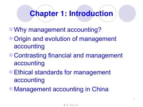
Chapter 1: Introduction
Why management accounting? Origin and evolution of management
accounting Contrasting financial and management
accounting Ethical standards for management
Accounting rate of return
17
第十八页，共七十三页。
Chapter 9 : The Operating Budget
Different approaches to budgeting

管理会计(英文版)课后习题答案(高等教育出版社)chapter 16

管理会计（高等教育出版社）于增彪（清华大学）改编余绪缨（厦门大学）审校CHAPTER 16COST-VOLUME-PROFIT ANALYSIS: A MANAGERIAL PLANNING TOOL QUESTIONS FOR WRITING AND DISCUSSION1.CVP analysis allows managers to focus onselling prices, volume, costs, profits, and sales mix. Many diffe rent “what if” questions can be asked to assess the effect on profits of changes in key variables.2.The units-sold approach defines sales vo-lume in terms of units of product and gives answers in these same terms. The sales-revenue approach defines sales volume in terms of revenues and provides answers in these same terms.3.Break-even point is the level of sales activitywhere total revenues equal total costs, or where zero profits are earned.4.At the break-even point, all fixed costs arecovered. Above the break-even point, only variable costs need to be covered. Thus, contribution margin per unit is profit per unit, provided that the unit selling price is greater than the unit variable cost (which it must be for break-even to be achieved).5.Profit = $7.00 ⨯ 5,000 = $35,0006.Variable cost ratio = Variable costs/Sales.Contribution margin ratio = Contribution margin/Sales. Contribution margin ratio = 1 –Variable cost ratio.7.Break-even revenues = $20,000/0.40 =$50,0008.No. The increase in contribution is $9,000(0.30 ⨯ $30,000), and the increase in adver-tising is $10,000.9.Sales mix is the relative proportion sold ofeach product. For example, a sales mix of3:2 means that three units of one productare sold for every two of the second product.10.Packages of products, based on the ex-pected sales mix, are defined as a singleproduct. Selling price and cost informationfor this package can then be used to carryout CVP analysis.11.Package contribution margin: (2 ⨯ $10) + (1⨯ $5) = $25. Break-even point = $30,000/$25= 1,200 packages, or 2,400 units of A and1,200 units of B.12.Profit = 0.60($200,000 – $100,000) =$60,00013. A change in sales mix will change the contri-bution margin of the package (defined by thesales mix) and, thus, will change the unitsneeded to break even.14.Margin of safety is the sales activity inexcess of that needed to break even. Thehigher the margin of safety, the lower therisk.15.Operating leverage is the use of fixed coststo extract higher percentage changes inprofits as sales activity changes. It isachieved by increasing fixed costs while lo-wering variable costs. Therefore, increasedleverage implies increased risk, and viceversa.16.Sensitivity analysis is a “what if” techniquethat examines the impact of changes in un-derlying assumptions on an answer. A com-pany can input data on selling prices, varia-ble costs, fixed costs, and sales mix and setup formulas to calculate break-even pointsand expected profits. Then, the data can bevaried as desired to see what impactchanges have on the expected profit.17.By specifically including the costs that varywith nonunit drivers, the impact of changesin the nonunit drivers can be examined. Intraditional CVP, all nonunit costs are lumpedtogether as “fixed costs.” While the costs arefixed with respect to units, they vary with re-spect to other drivers. ABC analysis remindsus of the importance of these nonunit driversand costs.18.JIT simplifies the firm’s cost equation sincemore costs are classified as fixed (e.g., di-rect labor). Additionally, the batch-level vari-able is gone (in JIT, the batch is one unit).Thus, the cost equation for JIT includes fixedcosts, unit variable cost times the number ofunits sold, and unit product-level cost timesthe number of products sold (or related cost driver). JIT means that CVP analysis ap-proaches the standard analysis with fixed and unit-level costs only.EXERCISES 16–11. e2. c3. d4. b5. a16–21. f2. d3. b4. a5. g6. e7. c16–31. Units = Fixed cost/Contribution margin= $10,350/($15 – $12)= 3,4502. Sales (3,450 ⨯ $15) $51,750Variable costs (3,450 ⨯ $12) 41,400Contribution margin $ 10,350Fixed costs 10,350Operating income $ 03. Units = (Target income + Fixed cost)/Contribution margin= ($9,900 + $10,350)/($15 – $12)= $20,250/$3= 6,7501. Contribution margin per unit = $15 – $12 = $3Contribution margin ratio = $3/$15 = 0.20, or 20%2. Variable cost ratio = $60,000/$75,000 = 0.80, or 80%3. Revenue = Fixed cost/Contribution margin ratio= $10,350/0.20= $51,7504. Revenue = (Target income + Fixed cost)/Contribution margin ratio= ($9,900 + $10,350)/0.20= $101,25016–51. 0.15($15)(Units) = $15(Units) – $12(Units) – $10,350$2.25(Units) = $3(Units) – $10,350$10,350 = $0.75(Units)Units = 13,8002. Sales (13,800 ⨯ $15) $ 207,000Variable costs (13,800 ⨯ $12) 165,600Contribution margin $ 41,400Fixed costs 10,350Operating income $ 31,050$31,050 does equal 15% of $207,000, so the answer of 13,800 units is correct.1. Before-tax income = (After-tax income)/(1 – Tax rate)= $6,000/(1 – 0.40)= $10,000Units = (Target income + Fixed cost)/Contribution margin= ($10,000 + $10,350)/($15 – $12)= 6,783**The answer is 6,783.3333, and so it must be rounded to a whole unit. You may prefer that students round up the answer to 6,784, instead, since it is better to be marginally above break-even than marginally below it.2. Before-tax income = (After-tax income)/(1 – Tax rate)= $6,000/(1 – 0.50)= $12,000Units = (Target income + Fixed cost)/Contribution margin= ($12,000 + $10,350)/($15 – $12)= 7,4503. Before-tax income = (After-tax income)/(1 – Tax rate)= $6,000/(1 – 0.30)= $8,571Units = (Target income + Fixed cost)/Contribution margin= ($8,571 + $10,350)/($15 – $12)= 6,30716–71. Break-even units = Fixed costs/(Price – Variable cost)= $150,000/($2.45 – $1.65)= $150,000/$0.80= 187,5002. Units = ($150,000 + $12,600)/($2.45 – $1.65)= $162,600/$0.80= 203,2503. Unit variable cost = $1.65Unit variable manufacturing cost = $1.65 – $0.17 = $1.48The unit variable cost is used in cost-volume-profit analysis, since it includes all of the variable costs of the firm.1. Before-tax income = $25,200/(1 – 0.40) = $42,000Units = ($150,000 + $42,000)/$0.80= $192,000/$0.80= 240,0002. Before-tax income = $25,200/(1 – 0.30) = $36,000Units = ($150,000 + $36,000)/$0.80= $186,000/$0.80= 232,5003. Before-tax income = $25,200/(1 – 0.50) = $50,400Units = ($150,000 + $50,400)/$0.80= $200,400/$0.80= 250,5004. 215,000 – 187,500 = 27,500 pansor$526,750 – $459,375 = $67,375A B C D Sales $ 5,000 $ 15,600* $ 16,250* $9,000 Variable costs 4,000 11,700 9,750 5,400* Contribution margin $ 1,000 $ 3,900 $ 6,500* $3,600* Fixed costs 500* 4,000 6,100* 750 Operating income (loss) $ 500 $ (100)* $ 400 $2,850 Units sold 1,000* 1,300 125 90 Price/unit $5 $12* $130 $100* Variable cost/unit $4* $9 $78* $60* Contribution margin/unit $1* $3 $52* $40* Contribution margin ratio 20%* 25%* 40% 40%* Break-even in units 500* 1,334* 118* 19* *Designates calculated amount.Note: When the calculated break-even in units includes a fractional amount, it has been rounded up to the next whole unit.16–101. Variable cost ratio = Variable costs/Sales= $399,900/$930,000= 0.43, or 43%Contribution margin ratio = (Sales – Variable costs)/Sales= ($930,000 – $399,900)/$930,000= 0.57, or 57%2. Break-even sales revenue = $307,800/0.57 = $540,0003. Margin of safety = Sales – Break-even sales= $930,000 – $540,000 = $390,0004. Contribution margin from increased sales = ($7,500)(0.57) = $4,275Cost of advertising = $5,000No, the advertising campaign is not a good idea, because the company’s o p-erating income will decrease by $725 ($4,275 – $5,000).1. Income = Revenue – Variable cost – Fixed cost0 = 1,500P – $300(1,500) – $120,0000 = 1,500P – $450,000 – $120,000$570,000 = 1,500PP = $3802. $160,000/($3.50 – Unit variable cost) = 128,000 unitsUnit variable cost = $2.2516–121. Contribution margin per unit = $5.60 – $4.20*= $1.40*Variable costs per unit:$0.70 + $0.35 + $1.85 + $0.34 + $0.76 + $0.20 = $4.20Contribution margin ratio = $1.40/$5.60 = 0.25 = 25%2. Break-even in units = ($32,300 + $12,500)/$1.40 = 32,000 boxesBreak-even in sales = 32,000 ⨯ $5.60 = $179,200or= ($32,300 + $12,500)/0.25 = $179,2003. Sales ($5.60 ⨯ 35,000) $ 196,000Variable costs ($4.20 ⨯ 35,000) 147,000Contribution margin $ 49,000Fixed costs 44,800Operating income $ 4,2004. Margin of safety = $196,000 – $179,200 = $16,8005. Break-even in units = 44,800/($6.20 – $4.20) = 22,400 boxesNew operating income = $6.20(31,500) – $4.20(31,500) – $44,800= $195,300 – $132,300 – $44,800 = $18,200 Yes, operating income will increase by $14,000 ($18,200 – $4,200).1. Variable cost ratio = $126,000/$315,000 = 0.40Contribution margin ratio = $189,000/$315,000 = 0.602. $46,000 ⨯ 0.60 = $27,6003. Break-even revenue = $63,000/0.60 = $105,000Margin of safety = $315,000 – $105,000 = $210,0004. Revenue = ($63,000 + $90,000)/0.60= $255,0005. Before-tax income = $56,000/(1 – 0.30) = $80,000Note: Tax rate = $37,800/$126,000 = 0.30Revenue = ($63,000 + $80,000)/0.60 = $238,333Sales ............................................................................... $ 238,333 Less: Variable expenses ($238,333 ⨯ 0.40) ................. 95,333 Contribution margin ...................................................... $ 143,000 Less: Fixed expenses ................................................... 63,000 Income before income taxes ........................................ $ 80,000 Income taxes ($80,000 ⨯ 0.30) ...................................... 24,000 Net income ................................................................ $ 56,0001. Operating income = Revenue(1 – Variable cost ratio) – Fixed cost(0.20)Revenue = Revenue(1 – 0.40) – $24,000(0.20)Revenue = (0.60)Revenue – $24,000(0.40)Revenue = $24,000Revenue = $60,000Sales ............................................................................... $ 60,000Variable expenses ($60,000 ⨯ 0.40) .............................. 24,000Contribution margin ...................................................... $ 36,000Fixed expenses .............................................................. 24,000 Operating income ..................................................... $ 12,000 $12,000 = $60,000 ⨯ 20%2. If revenue of $60,000 produces a profit equal to 20 percent of sales and if theprice per unit is $10, then 6,000 units must be sold. Let X equal number of units, then:Operating income = (Price – Variable cost) – Fixed cost0.20($10)X = ($10 – $4)X – $24,000$2X = $6X – $24,000$4X = $24,000X = 6,000 buckets0.25($10)X = $6X – $24,000$2.50X = $6X – $24,000$3.50X = $24,000X = 6,857 bucketsSales (6,857 ⨯ $10) ......................................................... $68,570Variable expenses (6,857 ⨯ $4) ..................................... 27,428Contribution margin ...................................................... $41,142Fixed expenses .............................................................. 24,000 Operating income ..................................................... $17,142 $17,142* = 0.25 ⨯ $68,570 as claimed*Rounded down.Note: Some may prefer to round up to 6,858 units. If this is done, the operat-ing income will be slightly different due to rounding.16–14 Concluded3. Net income = 0.20Revenue/(1 – 0.40)= 0.3333Revenue0.3333Revenue = Revenue(1 – 0.40) – $24,0000.3333Revenue = 0.60Revenue – $24,0000.2667Revenue = $24,000Revenue = $89,98916–151. Company A: $100,000/$50,000 = 2Company B: $300,000/$50,000 = 62. Company BX = $50,000/(1 – 0.80) X = $250,000/(1 – 0.40)X = $50,000/0.20 X = $250,000/0.60X = $250,000 X = $416,667Company B must sell more than Company A to break even because it must cover $200,000 more in fixed costs (it is more highly leveraged).3. Company A: 2 ⨯ 50% = 100%Company B: 6 ⨯ 50% = 300%The percentage increase in profits for Company B is much higher than Com-pany A’s increase because Company B has a higher degree of oper ating leve-rage (i.e., it has a larger amount of fixed costs in proportion to variable costs as compared to Company A). Once fixed costs are covered, additional reve-nue must cover only variable costs, and 60 percent of Company B’s revenue above break-even is profit, whereas only 20 perce nt of Company A’s revenue above break-even is profit.1. Variable Units in PackageProduct Price* –Cost = CM ⨯Mix = CM Scientific $25 $12 $13 1 $13 Business 20 9 11 5 55 Total $68 *$500,000/20,000 = $25$2,000,000/100,000 = $20X = ($1,080,000 + $145,000)/$68X = $1,225,000/$68X = 18,015 packages18,015 scientific calculators (1 ⨯ 18,015)90,075 business calculators (5 ⨯ 18,015)2. Revenue = $1,225,000/0.544* = $2,251,838*($1,360,000/$2,500,000) = 0.5441. Sales mix is 2:1 (Twice as many videos are sold as equipment sets.)2. Variable SalesP roduct Price –Cost = CM ⨯Mix = Total CM Videos $12 $4 $8 2 $16 Equipment sets 15 6 9 1 9 Total $25 Break-even packages = $70,000/$25 = 2,800Break-even videos = 2 ⨯ 2,800 = 5,600Break-even equipment sets = 1 ⨯ 2,800 = 2,8003. Switzer CompanyIncome StatementFor Last YearSales .......................................................................................... $ 195,000Less: Variable costs ................................................................. 70,000Contribution margin ................................................................. $ 125,000Less: Fixed costs ..................................................................... 70,000 Operating income ................................................................ $ 55,000 Contribution margin ratio = $125,000/$195,000 = 0.641, or 64.1%Break-even sales revenue = $70,000/0.641 = $109,2044. Margin of safety = $195,000 – $109,204 = $85,7961. Sales mix is 2:1:4 (Twice as many videos will be sold as equipment sets, andfour times as many yoga mats will be sold as equipment sets.)2. Variable SalesP roduct Price –Cost = CM ⨯Mix = Total CM Videos $12 $ 4 $8 2 $16 Equipment sets 15 6 9 1 9 Yoga mats 18 13 5 4 20 Total $45 Break-even packages = $118,350/$45 = 2,630Break-even videos = 2 ⨯ 2,630 = 5,260Break-even equipment sets = 1 ⨯ 2,630 = 2,630Break-even yoga mats = 4 ⨯ 2,630 = 10,5203. Switzer CompanyIncome StatementFor the Coming YearSales .......................................................................................... $555,000Less: Variable costs ................................................................. 330,000Contribution margin ................................................................. $225,000Less: Fixed costs ..................................................................... 118,350 Operating income ................................................................ $106,650 Contribution margin ratio = $225,000/$555,000 = 0.4054, or 40.54%Break-even revenue = $118,350/0.4054 = $291,9344. Margin of safety = $555,000 – $291,934 = $263,0661. Contribution margin/unit = $410,000/100,000 = $4.10Contribution margin ratio = $410,000/$650,000 = 0.6308Break-even units = $295,200/$4.10 = 72,000 unitsBreak-even revenue = 72,000 ⨯ $6.50 = $468,000or= $295,200/0.6308 = $467,977**Difference due to rounding error in calculating the contribution margin ratio.2. The break-even point decreases:X = $295,200/(P – V)X = $295,200/($7.15 – $2.40)X = $295,200/$4.75X = 62,147 unitsRevenue = 62,147 ⨯ $7.15 = $444,3513. The break-even point increases:X = $295,200/($6.50 – $2.75)X = $295,200/$3.75X = 78,720 unitsRevenue = 78,720 ⨯ $6.50 = $511,68016–19 Concluded4. Predictions of increases or decreases in the break-even point can be madewithout computation for price changes or for variable cost changes. If both change, then the unit contribution margin must be known before and after to predict the effect on the break-even point. Simply giving the direction of the change for each individual component is not sufficient. For our example, the unit contribution changes from $4.10 to $4.40, so the break-even point in units will decrease.Break-even units = $295,200/($7.15 – $2.75) = 67,091Now, let’s look at the break-even point in revenues. We might expect that it, too, will decrease. However, that is not the case in this particular example.Here, the contribution margin ratio decreased from about 63 percent to just over 61.5 percent. As a result, the break-even point in revenues has gone up.B reak-even revenue = 67,091 $7.15 = $479,7015. The break-even point will increase because more units will need to be sold tocover the additional fixed expenses.Break-even units = $345,200/$4.10 = 84,195 unitsRevenue = $547,26816–201.Break-even point = 2,500 units; + line is total revenue and x line is total costs.2. a. Fixed costs increase by $5,000:Break-even point = 3,750 unitsb. Unit variable cost increases to $7:Break-even point = 3,333 unitsc. Unit selling price increases to $12:Break-even point = 1,667 unitsd. Both fixed costs and unit variable cost increase:Break-even point = 5,000 units3. Original data:-$10,000$0$10,000Break-even point = 2,500 unitsa. Fixed costs increase by $5,000:-$15,000$0$15,000Break-even point = 3,750 unitsb. Unit variable cost increases to $7:-$10,000$0$10,000Break-even point = 3,333 unitsc.-$10,000$0$10,000Break-even point = 1,667 unitsd. Both fixed costs and unit variable cost increase:-$15,000$0$15,000Break-even point = 5,000 units4. The first set of graphs is more informative since these graphs reveal howcosts change as sales volume changes.1. Unit contribution margin = $1,060,000/50,000 = $21.20Break-even units = $816,412/$21.20 = 38,510 unitsOperating income = 30,000 ⨯ $21.20 = $636,0002. CM ratio = $1,060,000/$2,500,000 = 0.424 or 42.4%Break-even point = $816,412/0.424 = $1,925,500Operating income = ($200,000 ⨯ 0.424) + $243,588 = $328,3883. Margin of safety = $2,500,000 – $1,925,500 = $574,5004. $1,060,000/$243,588 = 4.352 (operating leverage)4.352 ⨯ 20% = 0.87040.8704 ⨯ $243,588 = $212,019New operating income level = $212,019 + $243,588 = $455,6075. Let X = Units0.10($50)X = $50.00X – $28.80X – $816,412$5X = $21.20X – $816,412$16.20X = $816,412X = 50,396 units6. Before-tax income = $180,000/(1 – 0.40) = $300,000X = ($816,412 + $300,000)/$21.20 = 52,661 units1. Variable Sales PackageP roduct Price –Cost = CM ⨯Mix = CM Vases $40 $30 $10 2 $20 Figurines 70 42 28 1 28 Total $48 Break-even packages = $30,000/$48 = 625Break-even vases = 2 ⨯ 625 = 1,250Break-even figurines = 6252. The new sales mix is 3 vases to 2 figurines.Variable Sales Package P roduct Price –Cost = CM ⨯Mix = CM Vases $40 $30 $10 3 $30 Figurines 70 42 28 2 56 Total $86 Break-even packages = $35,260/$86 = 410Break-even vases = 3 ⨯ 410 = 1,230Break-even figurines = 2 ⨯ 410 = 82016–231. d2. c3. a4. d5. e6. b7. cPROBLEMS16–241. Unit contribution margin = $825,000/110,000 = $7.50Break-even point = $495,000/$7.50 = 66,000 unitsCM ratio = $7.50/$25 = 0.30Break-even point = $495,000/0.30 = $1,650,000or= $25 ⨯ 66,000 = $1,650,0002. Increased CM ($400,000 ⨯ 0.30) $ 120,000Less: Increased advertising expense 40,000Increased operating income $ 80,0003. $315,000 ⨯ 0.30 = $94,5004. Before-tax income = $360,000/(1 – 0.40) = $600,000Units = ($495,000 + $600,000)/$7.50= 146,0005. Margin of safety = $2,750,000 – $1,650,000 = $1,100,000or= 110,000 units – 66,000 units = 44,000 units6. $825,000/$330,000 = 2.5 (operating leverage)20% ⨯ 2.5 = 50% (profit increase)16–251. Sales mix:Squares: $300,000/$30 = 10,000 unitsCircles: $2,500,000/$50 = 50,000 unitsSales Total Product P –V* = P – V ⨯ Mix = CM Squares $30 $10 $20 1 $ 20 Circles 50 10 40 5 200 Package $220 *$100,000/10,000 = $10$500,000/50,000 = $10Break-even packages = $1,628,000/$220 = 7,400 packagesBreak-even squares = 7,400 ⨯ 1 = 7,400Break-even circles = 7,400 ⨯ 5 = 37,0002. Contribution margin ratio = $2,200,000/$2,800,000 = 0.78570.10Revenue = 0.7857Revenue – $1,628,0000.6857Revenue = $1,628,000Revenue = $2,374,2163. New mix:Sales Total Product P –V = P – V ⨯ Mix = CM Squares $30 $10 $20 3 $ 60 Circles 50 10 40 5 200 Package $260 Break-even packages = $1,628,000/$260 = 6,262 packagesBreak-even squares = 6,262 ⨯ 3 = 18,786Break-even circles = 6,262 ⨯ 5 = 31,310CM ratio = $260/$340* = 0.7647*(3)($30) + (5)($50) = $340 revenue per package0.10Revenue = 0.7647Revenue – $1,628,0000.6647Revenue = $1,628,000Revenue = $2,449,2254. Increase in CM for squares (15,000 ⨯ $20) $ 300,000Decrease in CM for circles (5,000 ⨯ $40) (200,000)Net increase in total contribution margin $ 100,000Less: Additional fixed expenses 45,000Increase in operating income $ 55,000Gosnell would gain $55,000 by increasing advertising for the squares. This isa good strategy.16–261. Currently:Sales (830,000 ⨯ $0.36) $ 298,800Variable expenses 224,100Contribution margin $ 74,700Fixed expenses 54,000Operating income $ 20,700New contribution margin = 1.5 ⨯ $74,700 = $112,050$112,050 – promotional spending – $54,000 = 1.5 ⨯ $20,700Promotional spending = $27,0002. Here are two ways to calculate the answer to this question:a. The per-unit contribution margin needs to be the same:Let P* represent the new price and V* the new variable cost.(P – V) = (P* – V*)$0.36 – $0.27 = P* – $0.30$0.09 = P* – $0.30P* = $0.39b. Old break-even point = $54,000/($0.36 – $0.27) = 600,000New break-even point = $54,000/(P* – $0.30) = 600,000P* = $0.39The selling price should be increased by $0.03.3. Projected contribution margin (700,000 ⨯ $0.13) $91,000Present contribution margin 74,700Increase in operating income $16,300The decision was good because operating income increased by $16,300.(New quantity ⨯ $0.13) – $54,000 = $20,700New quantity = 574,615Selling 574,615 units at the new price will maintain profit at $20,700.16–271. P –V = P – V ⨯Mix = TotalResidential $540.00a$221.64c$318.36 2 $636.72 Commercial 160.00b124.52c35.48 1 35.48 Package $672.20 a$13.50 ⨯ 10 ⨯ 4b$40 ⨯ 4c Cost per acre for four applicationsCommercialChemicals $ 70.00 $ 70.00 [$40 + (3 ⨯ $10)] Labor* 80.00 18.00Operating expenses** 55.12 20.00Supplies** 16.52 16.52Total $ 221.64 $ 124.52*10/3 ⨯ $6.00 ⨯ 4; 3/4 ⨯ $6.00 ⨯ 4**The per-acre amount ⨯ 4 applicationsX = F/(P – V)= $39,708/$672.20 = 59* packagesResidential: 2 ⨯ 59 = 118 acresCommercial: 1 ⨯ 59 = 59 acresAverage number of residential customers = 118/0.10 = 1,180*Rounded2. Hours needed to service break-even volume (in packages):Residential: 10/3 ⨯ 4 ⨯ 2 = 26.67* hoursCommercial: 3/4 ⨯ 4 ⨯ 1 = 3.00 hours29.67 hours per packageTotal hours required = 29.67 ⨯ 59 = 1,751 hoursHours per employee = 8 ⨯ 140 = 1,120Employees needed = 1,751/1,120 = 1.6 laborersOne employee is not sufficient.Volume/Employee = 1,120/29.67 = 38 packages. Thus, if volume exceeds 38 composite units (76 residential and 38 commercial), a second laborer is needed (at least part time).*RoundedNote: Adding another employee could affect the costs used in the initial anal-ysis; for example: (1) another truck might be added (increasing fixed costs and the break-even point; (2) a two-man crew might be used (increasing variable costs); (3) the new employee might work evenings/weekends (no change in either fixed or variable costs). CVP used for planning is often an iterative process—the original solution may raise problems that may call for a recal-culation, altering plans further.3. The mix is redefined to be 1.2:0.8:1.0.P roduct P –V = P – V ⨯Mix = Total CM Res.-1 $135.00 $ 77.91* $ 57.09 1.2 $ 68.51 Res.-4 540.00 221.64 318.36 0.8 254.69 Comm. 160.00 124.52 35.48 1.0 35.48 Package $ 358.68 *Variable cost for one-time residential application:Chemicals $40.00Labor 20.00Operating expenses 13.78Supplies 4.13TotalX = F/(P – V) = $39,708/$358.68 = 111 packagesResidential (one application): 1.2 ⨯ 111 = 133 acresResidential (four applications): 0.8 ⨯ 111 = 89 acresCommercial: 1 ⨯ 111 = 111 acres1. Contribution margin ratio = $487,548/$840,600 = 0.582. Revenue = $250,000/0.58 = $431,0343. Operating income = CMR ⨯ Revenue – Total fixed cost0.08R/(1 – 0.34) = 0.58R – $250,0000.1212R = 0.58R – $250,0000.4588R = $250,000R = $544,9004. $840,600 ⨯ 110% = $924,660$353,052 ⨯ 110% = 388,357$536,303CMR = $536,303/$924,660 = 0.58The contribution margin ratio remains at 0.58.5. Additional variable expense = $840,600 ⨯ 0.03 = $25,218New contribution margin = $487,548 – $25,218 = $462,330New CM ratio = $462,330/$840,600 = 0.55Break-even point = $250,000/0.55 = $454,545The effect is to increase the break-even point.6. Present contribution margin $ 487,548Projected contribution margin ($920,600 ⨯ 0.55) 506,330Increase in contribution margin/profit $ 18,782Fitzgibbons should pay the commission because profit would increase by $18,782.1. Let X be a package of three Grade I cabinets and seven Grade II cabinets.Then:0.3X($3,400) + 0.7X($1,600) = $1,600,000X = 748 packagesGrade I: 0.3 ⨯ 748 = 224 unitsGrade II: 0.7 ⨯ 748 = 524 units2. P roduct P –V = P – V ⨯Mix = Total CMGrade I $3,400 $2,686 $714 3 $2,142 Grade II 1,600 1,328 272 7 1,904 Package $4,046 Direct fixed costs—Grade I $ 95,000Direct fixed costs—Grade II 95,000Common fixed costs 35,000Total fixed costs $ 225,000$225,000/$4,046 = 56 packagesGrade I: 3 ⨯ 56 = 168; Grade II: 7 ⨯ 56 = 3923. P roduct P –V = P – V ⨯Mix = Total CMGrade I $3,400 $2,444 $956 3 $2,868 Grade II 1,600 1,208 392 7 2,744 Package $5,612 P ackage CM = 3($3,400) + 7($1,600)P ackage CM = $21,400$21,400X = $1,600,000 – $600,000X = 47 packages remaining141 Grade I (3 ⨯ 47) and 329 Grade II (7 ⨯ 47)Additional contribution margin:141($956 – $714) + 329($392 – $272) $73,602Increase in fixed costs 44,000Increase in operating income $29,602Break-even: ($225,000 + $44,000)/$5,612 = 48 packages144 Grade I (3 ⨯ 48) and 336 Grade II (7 ⨯ 48)If the new break-even point is interpreted as a revised break-even for 2004, then total fixed costs must be reduced by the contribution margin already earned (through the first five months) to obtain the units that must be sold for the last seven months. These units would then be added to those sold during the first five months:CM earned = $600,000 – (83* ⨯ $2,686) – (195* ⨯ $1,328) = $118,102*224 – 141 = 83; 524 – 329 = 195X = ($225,000 + $44,000 – $118,102)/$5,612 = 27 packagesFrom the first five months, 28 packages were sold (83/3 or 195/7). Thus, the revised break-even point is 55 packages (27 + 28)—in units, 165 of Grade I and 385 of Grade II.。

《管理会计》（ManagementAccounting）课程教学大纲

《管理会计》（Management Accounting）课程教学大纲制定人：崔秀梅、殷俊明审核人：杨政第一部分课程概述一、基本信息（一）课程代码：02110090（二）课程属性、学分、学时《管理会计》是会计学、财务管理学、审计学等专业（本科）的一门专业必修课，主要讲授管理会计的基本理论和基本方法，阐述以提高经济效益为最终目的的会计信息利用系统，是为培养学生基本理论知识和应用能力而设置的一门专业课。

它将现代化管理与会计有机融为一体，向企业管理当局提供所需的会计信息，以便其有效地经营管理企业，制定企业政策，计划和控制企业活动，评价、选择决策方案，为企业提高经济效益服务。

学分：3 学时：48（三）适用对象适用于会计学、财务管理、审计学等专业的本科生。

二、课程简介《管理会计》将现代管理与会计融为一体，作为内部报告会计，向企业管理当局提供会计信息支持，以便其有效地经营管理企业，制定企业政策，计划和控制企业活动，评价决策方案，帮助企业实现其价值。

《管理会计》课程的内容主要包括四大知识模块：第一模块为管理会计基础篇部分，主要包括管理会计概述、成本性态的分析与应用、本量关系解析、变动成本法；第二模块为预测和决策部分，主要包括分部报告和分权制、短期经营决策；第三为规划和控制部分，主要包括全面预算管理、标准成本控制、作业成本管理；第四模块为责任与评价部分，主要包括责任会计和业绩评价。

Management accounting, as accounting for internal reporting, integrates modern management and accounting, providing accounting information to managers of enterprises to facilitate their management, decision-making, enterprise activities planning and evaluation scheme, for the purpose of realizing enterprise value.This course is divided into four parts. The first part is the fundamental knowledge of management accounting, including overview of accounting management, analysis and application of cost behavior, cost-volume-profit analysis andvariable costing. The second part deals with forecasting and decision-making, mainly including the segment reporting, system of decentralization, and short-term business decision. The third part is concerned with planning and control, covering comprehensive budgeting management, control of standard cost, and activity-based costing management.The last part is about responsibility and evaluation, including the responsibility accounting and performance evaluation.三、教学目标通过本课程的教学，使学生系统掌握现代管理会计的基本理论和基本方法，掌握预测、决策、全面预算、成本控制、责任考核评价等内容的技术方法和相关知识，并能将所学知识和操作技能，在社会主义市场经济条件下和现代企业制度环境中，应用于企业经营管理活动中，提高分析和解决企业经营管理问题的能力，为走向社会，加强企业管理、提高企业经济效益等方面发挥积极作用。

管理会计双语课件 Management accounting

03 作业
High-Tech
Globalization
Economic Transition
03 作业 Need for innovation and relevant produces: – Activity-based management • ABC Improves accuracy of assigning costs
– Customer orientation
• Strategic positioning to maintain competitive advantage
• Value chain framework to focus on customer value
– Total quality management emphasized continuous improvement
1950-1980 1980-
Most of the product-costing and internal accounting procedures used in the last century were developed.
Emphasis of accounting information for internal management . Management accounting practices developed, including: Flexible budgeting, Standard costs, Variance analysis, transfer prices et al.
03 管理会计的定义
1 、国外会计学界的定义 1 ）狭义管理会计管理会计知识为企业内部管理者提供规划和控制所需信息的内部会计。 • 为企业管理当局的管理目标服务。

《管理会计(双语)》课程 (5)

7
Time-Driven ABC
Use parameter estimates to assign indirect costs: Cost of using resource i by product j =
Capacity cost rate of resource i x Quantity of capacity of resource i used
Time-driven activity-based costing systems (TDABC or Time-Driven ABC) estimate two parameters and then assign indirect costs similar to the way direct costs are assigned
by product j
8
TDABC Profitability Report
Refer to Madison Dairy’s report, Exhibit 5-5 The results from the time-driven activity-based
costing system were quite different from the results based on the traditional cost system
Committed costs become variable via a two-st resources change either because of changes in the quantity of activities performed or because of changes in the efficiency of performing activities

金陵科技学院-管理会计（双语）管理会计复习提纲

PRACTICE QUESTIONS PART A, LECTURE 1QUESTION 3Answer the five questions below which relate to the following data: A firm had the following per unit costs for a period in which it expected to produce 1,000 units: DM $20, DL $30, Variable OH $20, Fixed OH $10, Variable selling costs $5 per unit. Answer the following costs related to the data:(a) Calculate the prime costs per unit.(b) Calculate the conversion costs per unit.(c) Calculate the product (inventoriable) cost per unit under absorption costing.(d) Calculate the variable product (inventoriable) cost per unit under absorption costing.(e) Calculate the period costs per unit.(f) Calculate the total expected costs if the firm produced and sold 1,100 units. Answer(a)Prime cost = DM + DL = $50 ($20 + $30)(b)Conversion cost = DL + OH = $60 ($30 + $20 + $10)(c)Product (inventoriable) cost under absorption costing = all manufacturing costs, i.e. $80 ($20 + $30 + $20 + $10)(d)V ariable product (inventoriable) cost under absorption costing = remove fixed OH of $10 per unit, therefore $70.(e)Period cost = all costs that are not manufacturing costs. Here, only selling costs, therefore $5.(f)Answer is $92,500, calculated as follows. Add total of expected manufacturing andnon-manufacturing costs. Note that the fixed and variable costs are treated differently: SOLUTIONS TO PRACTICE QUESTIONS, PART A LECTURE 2QUESTION 1Production budget for the month of AprilRequired for sales 1,000+ desired ending inventory 60 (5% x 1,200)1,060- opening inventory 52*Required production 1,008* If you did not know the actual inventory of products at the beginning of April (whether you do or not depends on how far in advance you are preparing the budgets), you would use the estimate for the beginning of April (which is the same as the end of March, i.e. 5% x 1,000 = 50).Direct Materials purchases budget for the month of April (in kgs)Required for production 2,016 (1,008 units x 2 kg)+ desired ending inventory 2002,216- opening inventory 125**Required purchases of material 2,091 kg** As before, if you did not know the actual inventory of materials at the beginning of April, you would use the estimate for the beginning of April (which is the same as the end of March, i.e. 250 kg)QUESTION 3Flexible budget formula is $100,000 + $40 per unit, therefore with no changes, budgeted costs would be: $100,000 + (20,000 x $40)= $900,000The effect of using overtime is that the variable cost will be greater than $40 per unit. Without further information, all we can conclude is that the budgeted amount will be some amount greater than $900,000.QUESTION 4A v. CM = (.1 x $4) + (.7 x $6) + (.2 x $2)= (.4 + 4.2 + .4) = $5BE point = 6,000 = 1,200 units in total, which is:5120 units of product 1 (10%)840 units of product 2 (70%)240 units of product 3 (20%)QUESTION 5(a)Cost A is not fixed, as it changes across activity levels. Not variable, because it is a different amount per unit at the different activity levels. Therefore it is mixed.Cost B is a fixed cost as in total it remains the same in total across different activity levels. Because Cost C is constant per unit across different activity levels, the total cost will vary in proportion to activity level, therefore it is a variable cost.(b)High cost – low costHigh activity – low activity$3,000-$2,0002,000-1,000= $1,000/1,000= $1 per unit.(c)Flexible budget formula for Cost A is $1,000 + $1 per unit.SOLUTIONS TO PRACTICE QUESTIONS, PART A, LECTURE 3QUESTION 2The following are summaries of the job cards for a particular period:Assume that only two jobs (#101 and #103) are finished, and job #103 is sold.(a) What is the balance of the WIP a/c and FG a/c at the end of the period, and the total expense for the period?(b) Is it possible to tell the total DM cost incurred for the period. If so, what is the amount?(c) Is it possible to tell the total DM cost EXPENSED during the period. If so, what is the amount?ANSWER(a) Identify which jobs are at different stages of the manufacturing and selling cycle, and therefore in each of the different accounts. Total the costs of those jobs. The total of the costs on the job cost sheets will be the balances of WIP and FG, and the total expense (amounta journal entry for all goods finished during the period.. However, at a particular point of time all jobs can be in one place only: either they are incomplete (WIP); finished and not sold (FG); or finished and sold (COGS).(b) Because the job cards indicate the opening balance for the period, all costs incurred in a previous period would be in the opening balance. Any costs itemised as DM, DL and OH on the job card are costs incurred this period. Therefore the cost of DM incurred for the periodis the total of the DM column, which is $96,000.(c)It would always be possible to find out the amount by going back through all the job cost sheets. In this example it is very easy to do because the opening balance is zero. Therefore, the amount of DM cost expensed during the period is the DM cost of any jobs sold. Job #103 was sold, and the DM cost of job #103 was $50,000.QUESTION 3Assume a firm started 5 jobs in a period. A summary of the costs on the job cost sheets∙Jobs 1, 2, 3 and 4 are finished in the period.∙Jobs 1 and 2 are sold in the period.∙Opening balances are zeroRequired:(a)Show the completed WIP, FG and COGS accounts.(b)What is the total amount of OH that has been applied during the period?(c)What is the amount of OH in the WIP account balance at the end of the period? ANSWER(a)WIPMaterials 150 FG 420 (jobs 1-4)Wages 200 Balance 180 (job 5)OH 250600 600FGWIP 420 COGS 150 (jobs 1-2)Balance 270 (jobs 3-4)420 420COGSFG 150(b) The total OH applied is found by adding OH on the job cost sheets for all jobs worked, i.e. $250.(c) The balance in any account consists of DM, DL and OH costs incurred on all jobs at that stage. There is only one job unfinished (job #5) therefore the balance in WIP of $180represents the costs incurred on job#5. We know from the job card that $70 of that cost is OH applied.QUESTION 4The following budgeted and actual results for a period relate to Dustin Pty Ltd, a firm which employs normal absorption job costing and applies OH using DL cost as the cost driver.Direct Manufacturing labour costs Manufacturing overhead costs Budget for 20071,000,0001,750,000Actual Results for 2007980,0001,862,000(a)Calculate the firm’s budgeted OH rate.(b)Calculate the cost of a particular job, job #323, which incurs $40,000 DM and $30,000 DL.(c)Calculate the amount of under/over applied overhead for the entire firm for the period, i.e. not just for job #323.ANSWER(a) 1,750,0001,000,000= 175% of DL cost or $1.75 for every dollar of DL.(b)Normal cost of job #323:DM $ 40,000DL $ 30,000OH $ 52,500 (175% of DL)$122,500(c)Total actual OH = $1,862,000Total applied OH = $1,715,000 (175% x $980,000)Under applied $ 147,000PRACTICE QUESTIONS, PART A, TOPIC 4QUESTION 2Calculate OH applied for the period given the following selected information:Budget information:Activity level 3,000 DL hoursV OH rate $3 per DL hourBudgeted total OH costs for actual activity level $15,900Actual data:Activity level 3,300 DL hoursANSWEROH applied will be actual hours worked x budgeted OH rates (both fixed and variable). What do we know?Actual hours worked = 3,300V ariable OH rate = $3 per DL hourWhat do we need to find?Fixed OH rate –this is not given. Recall that fixed OH rates can only be calculated at budgeted activity level. We know the budgeted activity level is 3,000, therefore the fixed OH rate will equal:Budgeted F OH (at budgeted activity)Budgeted activity level, i.e. 3,000Therefore, we need the budgeted F OH at budgeted activity level. But it is not given. All we are told is the total budgeted OH for actual activity, i.e. for 3,300 hours. We need to use this information to determine budgeted F OH, as follows:Total budgeted OH at 3,300 hours = $15,900V ariable budgeted OH at 3,300 hours = 3,300 x $3 = $9,900Therefore fixed budgeted OH at 3,300 hours = $15,900 - $9,900 = $6,000But if budgeted fixed OH at 3,300 hours is $6,000, budgeted fixed OH at 3,000 hours is also $6,000, so now we can work out the fixed OH rate, i.e.$6,000/3,000 = $2 per DL hour.We can now calculate OH applied, i.e. 3,300 x ($3+$2) = $16,500QUESTION 4A manufacturing firm has a direct labour cost of $25 per direct labour hour. Where jobs are worked in overtime hours, the cost is time-and-a-half, i.e. $37.50 per direct labour hour. A particular job was worked on for 8 hours, 4 hrs in normal time, and 4 hrs overtime.(a) What is the amount of overtime premium per DL hour?(b) What is the amount of overtime premium related to the job?(c) Show the journal entry for the labour cost assuming:(i) the overtime was necessary because of the particular nature of the job.(ii) the overtime was necessary because of poor scheduling by the firm.Answer(a)The premium is $12.50 per DL hour.(b)4 hours x $12.50 = $50.(c) (i)WIP DR 250Wages and Salaries Payable CR 250(in these circumstances the overtime premium is charged to the job, and therefore ends up in the WIP account, and eventually in FG account).(ii)WIP DR 200OH DR 50Wages and Salaries Payable CR 250(in these circumstances the overtime premium is not charged to the job. Only the ordinary costs per hour ($25) for the hours worked on the job are charged to WIP.)SOLUTIONS TO PRACTICE QUESTIONS, PART A, TOPIC 5(a) Calculate the labour rate variance and the labour efficiency variance, using either tables or formulae.(b) Show the journal entry required to record labour information for the period.(c) Calculate the material price variance and the material efficiency variance (using either tables or formulae) assuming the MPV is isolated on purchase.(d) Show the journal entries for materials purchased and used.(e) Repeat (c) and (d) assuming MPV is isolated on usage. This means you are to recalculate the MPV, and show the journal entries for purchase and use of material for this option.AnswerUsing formulae:LRV = 770 x ($32 - $30) = +$1,540 = $1,540 ULEV = $30 x (770 – 725) = -$1,350 = $1,350 UPart (c)Using formulae:MPV = 4,000 x ($10.50 - $10) = +$2,000 = $2,000 UMEV = $10 (3,100 – 2,900) = +$2,000 = $2,000 UPart (e)Using formulae:MPV = 3,100 x ($10.50 - $10) = +$1,550 = $1,550 UQUESTION 3“Fit to a T” designs and manufactures T-shirts, and sells them in one-dozen lots. A new type of material was purchased in the period, which led to faster cutting and sewing but the workers used more material than usual as they learned to work with it. The following are selected budget and actual results for the period:Static BudgetNumber of T-shirt lots (1 lot = 1 dozen) 500Per lot of T-shirts:Direct materials 12 metres at $1.50 per meter = $18.00Direct manufacturing labour 2 hours at $8.00 per hour = $16.00Actual resultsNumber of T-shirt lots sold 550Total direct inputs:Direct materials 7,260 metres at $1.75 per meter = $12,705 Direct manufacturing labour 1,045 hours at $8.10 per hour = $8,464.50(a) Calculate the direct material and direct labour variances for the period.(b) Identify possible reasons (suggested from the facts given only – not the general ones in the lecture notes) for the efficiency variances you have calculated.Answer(a) Direct MaterialsAQ used x AP AQ used x SP SQ x SP7,260 x 1.75 7,260 x 1.50 (550 x 12) x 1.5012,705 10,890 6,600 x 1.509,900MPV MEV$1,815 U $990 UFLEXIBLE BUDGET V ARIANCE$2,805 UDirect LabourAQ used x AP AQ used x SP SQ x SP1,045 x 8.10 1,045 x 8 (550 x 2) x 88,464.50 8,360 1,100 x 88,800LRV LEV$104.50 U $440 FFLEXIBLE BUDGET V ARIANCE$335.50 FTOTAL FLEXIBLE BUDGET V ARIANCE$2,469.50 U ($2,805 - $335.50)(b) Possible reasons for efficiency variances (using only facts given):Unfavourable MEV because the new type of material was di fferent to work with, therefore the workers wasted more material than usual while getting used to its different texture etc. Favourable LEV because we are told that the material resulted in “faster cutting and sewing”.AYB225 – PRACTICE QUESTIONS, LECTURE 7QUESTION 1Standard manufacturing costs per unit: (Unchanged from previous accounting period)DM $6; DL $4; V OH $3; F OH $2Physical quantities: (There were no WIP inventories.)Opening FG - 300Units produced - 6,000Closing FG - 200Other cost and price data:Selling price per unit - $25Actual F OH - $11,500Selling and admin costs - $5,000 Fixed, $3,000 V ariable.Variances for the period:Total variable (DM, DL, V OH) - 15,000 UTotal fixed – 500 FRequired:(a) Properly classified Absorption Costing Income Statement for the period.(b) Properly classified V ariable Costing Income Statement for the period.(c) Quantitatively reconcile the profits under the two systems.(d) Explain why the AC profit is less than DC profit.ANSWERAC product cost per unit is 6+4+3+2 = $15DC product cost per unit is 6+4+3 = $13(a) Absorption Costing Income StatementSales (6,100 x $25) 152,500Less Cost of Goods Sold:(6,100 x $15) 91,500Add net variances (unfavourable) 14,500 106,000GROSS MARGIN 46,500Less Selling and Administrative Expenses 8,000NET PROFIT $38,500(b) Direct Costing Income StatementSales (6,100 x $25) 152,500Less V ariable Costs;COGS (6,100 x $13) 79,300Add net variances (unfavourable) 15,000 94,300Selling and Administrative Expenses 3,000 97,300 CONTRIBUTION MARGIN 55,200Less Fixed Costs:Overhead 11,500Selling and Administrative 5,000 16,500NET PROFIT $38,700(c)Inventory decreased from 300 to 200, therefore:Change in inventory 100 x F OH per unit ($2) = $200 explains the difference in profit. Because the fixed OH per unit is unchanged from the previous period, it is possible to conclude that because inventory has decreased profit under AC will be $200 smaller than under DC.(d)The total fixed OH incurred and expensed under DC relates to the 6,000 units produced. Under AC the firm expenses the amount of F OH relating to units sold, which is 6,100. Therefore, because the firm produced less than it sold, under AC an additional amount of fixed OH is expensed which relates to the units in opening inventory. (The full explanationis actually more complicated than this explanation, but the above is all that you are required to know for this unit.AYB225 – SOLUTIONS, PRACTICE QUESTIONS LECTURE 8Note: If you are required to complete a cost of production report in the examination you will be provided with a pro-forma.QUESTION 1 (a)Calc. EUOpening WIP 50%Transferred InTo A/c forCompletedClosing WIP (75%)A/c forCalc. Unit CostsWIPCurrentCosts to Account ForEUUNIT COSTSAllocation of CostsGoods Completed8,000 x $10.2091 81,673Work in process3,000 x 2.9091 8,7273,000 x 2.9 8,7000 x .80 02,250 x 3.60 8,100 25,527107,200* In practice the journal entries would separate out these amounts, as the solution does. If you know the figures, you must show them separately.(c)Work in Process – 2 a/cBalance 44,800 To FG 81,673WIP-1 20,000 Close bal 25,527 (this agrees with the amount above)Material X 16,000Material Y 6,400Payroll 14,000OH 6,000107,200 107,200QUESTION 2(a) COST OF PRODUCTION REPORTCalc. EUOpening WIP 40%Transferred InTo A/c forCompletedClosing WIP(60%)A/c forCalc. Unit CostsWIPCurrentCosts to Account ForEUUNIT COSTSAllocation of CostsGoods Completed2,000 x 83.004 $166,008WIP 400 x 49.104 T/I 19,642240 X 25 CC 6,000 $ 25,642$191,650(b) Work in Process - Spinning Department $96,000Work in Process - Drawing Department $96,000Work in Process – Spinning $ 63,800Materials $ 17,800Payroll, Misc. Credits (if known list separately) $ 46,000Finished Goods $166,008Work in Process - Spinning Department $166,008AYB225 – PRACTICE QUESTIONS, LECTURE 9COST ALLOCATIONPART A – SERVICE DEPARTMENT ALLOCATIONQUESTION 1A firm has two production departments, Mixing and Finishing. These departments areserviced by two support departments, Administration and Payroll. The costs and % usage of the service departments follows:(b) Calculate the billing rates per work unit for administration and payroll under the directmethod, assuming that 1% = 1 work unit. Round to 2 decimal places.(c) Show the allocation using the step-down method, starting with Administration.(d) Show the allocation using the step-down method, starting with Payroll.(e) Calculate the billing rates per work unit for administration and payroll for the methodused in (d) assuming that 1% = 1 work unit. Round to 2 decimal places.FromAdministration From Payroll(b) Administration = 60,000/80 = $750 per unit of work Payroll = 80,000/70 = $1,142.86 per unit of work(c) - STEPFromAdministration From Payroll(d)From PayrollFromAdministration(e) Administration = 84,000/80 = $1,050 per work unit Payroll = 80,000/100 = $800 per work unitQUESTION 1Daniel Supply Company manufactures three products. The first process is a joint process, with joint costs of $127,500. Opening WIP and FG inventory are(a) Show three (3) different “physical measures method” allocations of joint costs using the above data.Note: Joint cost allocation must be based on units produced, NEVER units sold.(b) Show joint cost allocation for Daniel Supply Company assuming the net realisable value method.(c) Use the data for Daniel Supply Company above, except assume now that Bizmo is a by-product.Show the allocation of the joint costs assuming the net realisable value method, and:(i)the net realisable value of the by-product is treated as miscellaneous income.(ii)(ii) the net realisable value of the by-product reduces the costs of the principal products.ANSWER(a)One method would be to say there are three products, therefore each product will be allocatedAnother would be based on the number of physical units produced. The firm produced the following number of units through the joint process:A third would be based on the weighted units produced, i.e.Note that under the three different ways to interpret “physical method”, the amounts are different, and so is the direction in terms of which products are allocated the higher cost.(c)Note: Use the proportions of NRV calculated in part (b) above, i.e. Gizmo 630, Wizmo 280(i) Under this method the total joint costs are allocated to the products only (i.e. not to by-product Bizmo):NRV AllocationGizmo 630 630/910 $ 88,269Wizmo 280 $ 39,231$127,500(ii) Under this method the joint costs are reduced by the net realisable value of Bizmo, i.e. $127,500 less ($40,000 less $8,000) = $95,500. These costs are then allocated to the products only (i.e. not to by-product Bizmo):NRV AllocationGizmo 630 630/910 $66,115Wizmo 280 $29,385$95,500。

财会专业英语-中英文对照

AAbsorption costing 完全成本法Accelerated Depreciation Method 加速折旧法Account 科目,账户Account form 账户式Account payable 应付账款Account receivable 应收账款Accounting 会计Accounting cycle 会计循环Accounting equation 会计等式资产 Assets= 负债 Liabilities + 所有者权益Owner’s EquityAccounting period concept 会计期间Accounting system 会计制度Account payable subsidiary ledger 应付款明细分类账Accounts receivable analysis 应收账款分析Accounts receivable subsidiary ledger 应收账款明细分类账Accounts receivable turnover 应收账款周转率Accrual basis accounting 应记制，债权发生制Accrued expenses 应记费用Accrued revenues 应记收入Accumulated depreciation 累计折旧Accumulated other comprehensive income 累计其他综合收入Activity base drive 作业基础/动因Activity—based costing ABC 作业成本计算法Adjusted trial balance调整后试算平衡表Adjusting entries调整分录Adjusting process调整过程Administrative expenses general expenses管理费用一般费用Aging the receivables应收账款账龄分析Allowance for doubtful accounts 坏账准备Allowance method备抵法Amortization摊销Annuity年金Assets资产Available—for—sale securities可供出售证券Average inventory cost flow method 平均库存成本流法Average cost method平均成本法Average rate of return平均回报率BBad debt expense 坏账费用Balance of the account账户余额Balance sheet资产负债表Balanced scorecard平衡记分卡Bank reconciliation银行存款余额调节表Bank statement 银行报表Bond债券Bond indenture债券契约Book value账面价值Book value of the asset资产的账面价值Boot补价Break-even point盈亏临界点Budget预算Budget performance report预算业绩报告Budgetary slack预算松弛Budgeted variable factory overhead 预算变量工厂开销Business企业Business combination 企业合并Business entity concept企业主体概念Business stakeholder企业利益相关者Business strategy企业战略Business transaction经济业务CCapital account 资本性账户Capital expenditures资本性支出Capital expenditures budget资本支出预算Capital investment analysis资本投资分析Capital leases资本性租赁Capital rationing资本分配Carrying amount账面金额Cash现金Cash basis of accounting现金制；收付实现制Cash budget现金预算Cash dividend现金股利Cash equivalents现金等价物Cash flow per share 每股现金流量Cash flows from financing activities筹资活动现金流量Cash flows from investing activities投资活动现金流量Cash flows from operating activities经营活动现金流量Cash payback period现金回收期Cash payments journal现金付款日记账Cash receipts journal现金收款日记账Cash short and over account现金余缺账户Certified public accountant CPA注册会计师Chart of accounts会计科目表Clearing account 清理账户Closing entries结账分录Closing process结账程序Closing the books 结账Common stock普通股Common—size statement通用报表Compensating balance 补偿性余额Comprehensive income全面收益Consigned inventory 寄售库存Consignee 收货人承销人Consignor 发货人寄件人Consolidated financial statements合并财务报表Contingent liabilities 不确定债务Continuous budgeting滚动预算Continuous process improvement 持续过程改进Contra accountor contra asset account抵减账户Contract rate约定利率Contribution margin 贡献毛益Contribution margin ratio贡献毛益率Contribution margin ratio 边际贡献率Controllable expenses可控费用Controllable revenues 可控收入Controllable variance可控差异Controller主计长Controlling 管理控制Controlling account控制账户Conversion costs加工成本Copyright版权Corporation公司Correcting journal entry 调整分录Cost成本Cost accounting system成本会计系统Cost allocation成本分配Cost behavior成本性态Cost center成本中心Cost concept 成本概念Cost method 成本法Cost object 成本对象Cost of finished goods available 已完工产品的成本Cost of goods manufactured 产品成本Cost of goods sold产品销售成本Cost of goods sold budget产品销售成本预算Cost of merchandise sold商品销售成本：商业企业所销售商品的成本.Cost of merchandise purchased 产品购买成本Cost of merchandise sold 销货成本Cost of production report 生产成本报告Cost per equivalent unit单位约当产量成本Cost price approach成本价格法Cost variance成本差异Cost-volume-profit analysis本－量－利分析Cost-volume-profit chart本－量－利图Credit memorandumcredit memo贷项通知单Credit period 贷款期限Credit terms 赊销付款条件，信用证条款Credits 贷记Cumulative preferred stock累积优先股Currency exchange rate货币汇率Current assets流动资产Current liabilities流动负债Current position analysis 流动财务状况分析Current ratio流动比率Currently attainable standards当前可达标准DDebit memorandum 借项通知单Debits借记debt securities债务证券，债券decision making 决策，判定；作出判定Deficiency 亏损Deficit 亏损Defined benefit plan 固定收益计划：Defined contribution plan 固定缴款计划：Depletion 折耗：Depreciate：贬值Depreciation 资产等折旧;货币贬值；跌价Depreciation expense 折旧费用Differential analysis 差异分析Differential income or less 差别收入或更少Differential cost 差异成本Differential revenue 差异收入Differential strategy 差异化战略Direct labor cost 直接人工成本Direct labor cost budget 直接人工成本预算Direct labor rate variance 直接人工工资率差异Direct labor time variance 直接人工工时差异Direct materials cost 直接材料成本Direct materials price variance 直接材料价格差异Direct materials purchases budget 直接材料采购预算Direct materials quantity variance 直接材料数量差异Direct method 直接法：Direct write—off method 直接注销法:Directing 指导Discount 贴现息；折价：Dishonored note receivable 拒付应收票据：Dividend yield 股利收益率：Dividends 股息，红利Dividends per share每股股利Double-declining—balance method双倍余额递减法Double—entry accounting system 复式会计模式：Drawing 提款：DuPont formula 杜邦公式EEarnings per common share EPS on common stock 普通股每股收益E—commerce 电子商务：Effective interest rate method 实际利率法Effective rate of interest 实际利率：债券发行时的市场利率。

管理会计经典书籍

管理会计经典书籍管理会计是指应用会计理论和技术进行企业管理决策的一门学科。

下面是一些经典的管理会计书籍，它们涵盖了管理会计的各个方面，对于理解管理会计的概念和应用具有重要的意义。

1.《管理会计：信息和决策导向》（Management Accounting: Information for Decision-Making）- 作者：Anthony A. Atkinson, Robert S. Kaplan, Ella Mae Matsumura, S. Mark Young这本书是管理会计领域的经典之作，全面介绍了管理会计的基本概念、技术和应用。

它强调了管理会计在决策制定和绩效评估中的重要性，提供了实用的工具和方法来帮助管理者做出明智的决策。

2.《管理会计：信息与策略》（Management Accounting: Information for Strategy）- 作者：Anthony A. Atkinson, Robert S. Kaplan, Ella Mae Matsumura, S. Mark Young这本书进一步探讨了管理会计与战略管理之间的关系。

它介绍了如何使用管理会计信息来支持战略决策，并提供了一些实用的案例分析来说明理论的应用。

3.《成本与管理会计》（Cost and Management Accounting）- 作者：Colin Drury这本书主要关注成本会计和管理会计的理论和实践。

它介绍了成本的概念、分类和计算方法，以及如何使用成本信息来做出管理决策。

4.《管理会计与绩效管理》（Management Accounting and Performance Management）- 作者：Martin Quinn, Ron Carroll这本书着重介绍了管理会计在绩效管理中的应用。

它探讨了如何制定和评估绩效目标，并使用管理会计信息来监控和改进绩效。

5.《管理会计与战略成本管理》（Management Accounting and Strategic Cost Management）- 作者：Mohammad R. Daftari这本书介绍了管理会计和战略成本管理的理论和实践。

财务管理专业英语_PDF图书下载_刘媛媛编_在线阅读_PDF免费电子书下载_第一图书网（5篇模版）

财务管理专业英语_PDF图书下载_刘媛媛编_在线阅读_PDF免费电子书下载_第一图书网（5篇模版）第一篇：财务管理专业英语_PDF图书下载_刘媛媛编_在线阅读_PDF 免费电子书下载_第一图书网财务管理专业英语_PDF图书下载_刘媛媛编_在线阅读_PDF免费电子书下载_第一图书网前言A journey of a thousand miles begins with a single step.——Chinese proverb The future is not what it used to be.——Paul Valery 21世纪是一个竞争激烈、国际化的高科技时代，21世纪的高级专门人才要具备扎实的专业知识、较高的信息素养和能在专业领域用外语进行交流沟通的能力。

作为一名财务管理专业教师，近几年来，我一直采用国外原版教材从事财务管理专业和非财务管理专业的财务管理课程的双语教学。

我深切体会到，虽然学生已经系统学习了大学基础英语，但由于缺乏专业英语基础，财务管理双语课程的教学效果并不尽如人意。

因此，很有必要在财务管理专业教学中设置财务管理专业英语课程。

财务管理专业英语教学，作为从基础英语教学向专业课双语教学过渡的桥梁，是财务管理专业学生从基础英语学习向专业领域英语应用过渡的不可或缺的中间环节。

要对学生进行财务管理专业英语素养的培养，一本合适的财务管理专业英语教材就成为至关重要的因素。

本书从财务管理专业培养目标出发，力求成为一本实用的财务管理专业英语教材，并采用有助于提高学生专业知识和实际运用能力的编写形式，以期能使学生成为满足日益激烈的国际竞争和频繁的国际交流需求的高素质财务管理人才。

本书按财务管理专业主干课程的架构分为12个专题，分别介绍财务管理各个方面的专业英语基础知识。

每一专题均先以“名人名言”和“微型案例”开始，以激发学生的兴趣去主动获取知识、开阔视野。

正文尽量体现财务管理专业的基本理念与核心内容，每一专题还设有“知识扩展”、“相关网址”等，进一步丰富了教学内容。

财务管理系课程介绍(中英对照)

财务管理系课程介绍（中英对照）序号：1课程编码：11001030、11001020课程名称：管理会计Management Accounting学分：3周学时： 3开课系部：财务管理系预修课程：会计学基础、财务会计修读对象：本科生课程简介：本课程是财务管理专业的专业方向课，主要介绍管理会计的基本理论，及如何运用会计及其它经营信息，对企业经济活动进行规划、控制、评价和考核；其主要内容包括：本量利分析、预测分析、投资决策、全面预算、成本控制与标准成本系统、责任会计等。

拟用教材：《管理会计》，毛付根主编，高等教育出版社2000年版参考教材：《管理会计》，余绪缨主编，中国人民大学出版社 1999年版；《管理会计学》（英文版），Ronald W. Hiltion主编，机械工业出版社 2000年版；《管理会计应用与发展的典型案例研究》，潘飞主编，中国财政经济出版社 2002年版Course Code: 11001030、11001020Course Title: Management AccountingDepartment: Financial Management Dept.Credit: 3Periods per week: 3Preparatory Course: Fundamental Accounting, Financial AccountingStudents: UndergraduatesContents:This is a core course for the students whose major is Financial Management. This course introduces the basic theories of management accounting system and itsapplication in the operational activities such as planning, control, evaluation,performance assessing of a business enterprise. The topics covered includecost-volume-profit analysis, business forecasting and its analysis, long-terminvestment decisions making (capital budgeting), master budgeting, cost controland standard costing system, responsibility accounting, etcCourse Book: Mao fugen. Ed. 2000. Managerial Accounting, Higher Education Press Reference Book:Yu Xuying. Ed. 1999. Managerial Accounting, China RenMin University Press;Ronald W. Hiltion. Ed. 2000. Managerial Accounting (English version), ChinaMachine Press; Pan Fei. Ed. 2000. Managerial Accounting Application andDevelopment and Typical Cases Analysis, The Chinese Finance and EconomicsPublishing House.序号： 2课程编码：11002040课程名称：财务管理Financial Management学分： 4周学时：4开课系部：财务管理系预修课程：会计学基础、财务会计修读对象：本科生课程简介：本课程是财务管理专业的专业方向课，主要介绍现代财务管理的基本理论和方法及其具体应用。

管理会计双语测试题

管理会计双语测试题Managerial Accounting Review Question⼀、True/False QuestionsFor each of the following, circle the T or the F to indicate whether the statement is true or false.1Managerial accounting refers to the preparation and use of accounting information designed to meet the needs of decision makers inside the business organization.2Product costs are selling expenses that appear on the income statement.3Management accounting reports provide a means of monitoring , evaluating and rewarding performance.4Product costs are offset against revenue in the period in which the related products are sold, rather than the period in which the costs are incurred.5Manufacturing overhead is considered an indirect cost, since overhead costs generally cannot be traced conveniently and directly to specific units of product.6Overhead application rates allow overhead to be assigned at the beginning of a period to help set prices.7Pepsi Cola would most likely use a job order costing system.8Activity-based costing tracks cost to the activities that consume resources.9Activity based costing uses multiple activity bases to assign overhead costs to units of production.10The two steps required in Activity Based Costing are 1) Identify separate activity cost pools and 2) allocate each cost pool to the product using an appropriate cost driver11The new manufacturing environment is characterized by its shift toward labor intensive production and declining manufacturing overhead costs.12A cost driver is an activity base that is highly correlated with manufacturing overhead costs.13In ABC, only one cost driver should be used in applying overhead.14As companies become more automated overhead costs decrease and direct labor costs increase.15An equivalent unit measures the percentage of a completed units cost that is present in a partially finished unit.16Costs do not flow through a process cost system in the same sequence as actual products move through the assembly process.17Non-value added activities are those that do not add to a product's desirability.18Target costing centers on new product and service development as opposed to managing the value chain for existing products.19In the target costing process, target price is computed by adding the desired profit margin to the target product cost.20Target cost equals target price plus profit margin.21Variable costs which increase in total amount in direct proportion to an increase in output represent a constant amount per unit of output.22Any business which operates at less than capacity will have larger fixed costs than variable costs.23With variable costs, the cost per unit varies with changes in volume.24The contribution margin is the difference between total revenue and fixed costs.25The volume of output which causes fixed costs to be equal in amount to variable costs is called the break-even point.26Any business which operates at less than capacity will have larger fixed costs than variable costs.27Margin of safety is the dollar amount by which actual sales volume exceeds the break-even sales volume.28Life cycle costing considers all potential resources used by the product over its entire life.29Economies of scale can be achieved by using facilities more intensively.30The break-even point is the level of activity at which operating income is equal to cost of goods sold.31Contribution margin ratio is equal to contribution margin per unit divided by unit sales price.32Opportunity cost is the benefit that could have been obtained by pursuing an alternate course of action.33All incremental revenue or incremental costs are relevant.34Sunk costs are relevant to decisions about replacing plant assets.35In determining whether to scrap or to rebuild defective units of product, the cost already incurred in producing the defective units is not relevant.36In making a decision, management will look thoroughly at both relevant and irrelevant data.373.Responsibility margin is useful in evaluating the consequences of short-run marketing strategies, while contribution margin is more useful in evaluating long-term profitability.38The transfer price is the dollar amount used in recording sales to primary customers.39Under variable costing, fixed manufacturing costs are treated as period costs, rather than product costs.40The transfer price is the dollar amount used in recording sales to primary customers.41Variable costing treats all fixed manufacturing costs as expenses of the current period.42In full costing when production rises above the amount of sales, some of the fixed costs will remain in inventory.43Return on Investment (ROI) tells us how much earnings can be expected for the average invested dollar.44Capital turnover can be improved by reducing invested capital while keeping sales constant.45The value chain consists of only those activities that increase the selling price of a product as it is distributed to a customer.46Residual income is calculated by subtracting the minimum acceptable return on the average invested capital from the operating income.⼆、Multiple Choice QuestionsChoose the best answer for each of the following questions and insert the identifying letter in the space provided.1.Costs that are traceable to a particular unit and are inventoriable are calledA) Period costs B) Product costs C) Overhead costs D) Job costs2. .Determine the amount of manufacturing overhead given the following information:a. Depreciation on a factory building $2,400b. Telephone expense in factory office750c. Telephone expense in sales showroom850d. Factory foreman’s salary5000e. Maintenance for factory` 800f. Maintenance for sales showroom 680A) $4,010 B) $9,800 C) $8,950 D) $10,54024.Goods that are still in the production process would be in which account?A) Materials inventory B) Work-in-process inventory C)Finished goods inventory D)Cost of goods sold29.The principal difference between managerial accounting and financial accounting is that managerial accounting information is:A) Prepared by managers.B) Intended primarily for use by decision makers inside the business organization.C) Prepared in accordance with a set of accounting principles developed by the Institute of CertifiedManagerial Accountants.D) Oriented toward measuring solvency rather than profitability.30.Management accounting systems are designed to assist organizations in the performance of all of the following functions except:A) The assignment of decision-making authority over company assets.B) Planning and decision-making.C) Monitoring, evaluating and rewarding performance.D) The preparation of income tax returns.35.In comparison with a financial statement prepared in conformity with generally accepted accounting principles, a managerial accounting report is less likely to:A) Focus upon the entire organization as the accounting entity. B) Focus upon future accounting periods.C) Make use of estimated amounts. D) Be tailored to the specific needs of an individual decision maker.4.If the salaries of the sales staff of a manufacturing company are improperly recorded as a product cost, what will be the likely effect on net income of the period in which the error occurs?A) Net income will be overstated. B) Net income will be understated.C) Net income will be unaffected. D) Net income will be understated only if inventory levels rise.5.Manufacturing overhead is best described as:A) All manufacturing costs other than direct materials and direct labor.B) All period costs associated with manufacturing operations.C) Indirect materials and indirect labor.D) All operating expenses other than selling expenses and general and administrative expenses.43.Underapplied overhead at the end of a month:A) Results when actual overhead costs are less than amounts applied to work in process.B) Indicates a poorly designed cost accounting system.C) Is represented by a debit balance remaining in the Manufacturing Overhead account.D) Is represented by a credit balance remaining in the Manufacturing Overhead account.58.The account Work-in-Process InventoryA) Consists of completed goods that have not yet been soldB) Consists of goods being manufactured that are incompleteC) Consists of materials to be used in the production processD) Consists of the cost of new materials used, labor but not overhead.66.Red Star Company uses a job order cost system. Overhead is applied to jobs on the basis of direct labor hours.During the current period, Job No. 288 was charged $400 in direct materials, $450 in direct labor, and $180 in manufacturing overhead. If direct labor costs an average of $15 per hour, the company's overhead application rate is:A) $9 per direct labor hour. B) $6 per direct labor hour.C) $17 per direct labor hour. D) $20 per direct labor hour.24.The best cost system to use for a company producing a continuous stream of similar items would be aA) Job order system B) Process costing system C) Production costing systemD) No cost system is required when jobs are similar64.Ken Gorman’s Company uses a job order cost system and has established a predetermined overhead application rate for the current year of 150% of direct labor cost, based on budgeted overhead of $900,000 and budgeted direct labor cost of $600,000. Job no. 1 was charged with direct materials of $30,000 and with overhead of $24,000.The total cost of job no. 1:A) Is $54,000. B) I s $70,000. C)Is $90,000. D) Cannot be determined without additional information.27.Equivalent units of production areA) A measure representing the percentage of a unit's cost that has been completed.B) May be computed separately for each input added during productionC) May be assigned to beginning work-in-process or ending work-in-processD) All of the above27.Equivalent units of production areA) A measure representing the percentage of a unit's cost that has been completed.B) May be computed separately for each input added during productionC) May be assigned to beginning work-in-process or ending work-in-processD) All of the above21.Process costing would be suitable forA) Automobile repair B) Production of television sets C) Boat building D) K itchen remodeling Use the following to answer questions 75-76:Riverview Company's budget for the coming year includes $6,000,000 for manufacturing overhead, 100,000 hours of direct labor, and 500,000 hours of machine time.75. Refer to the above data. If Riverview applies overhead using a predetermined rate based on machine-hours,what amount of overhead will be assigned to a unit of output which requires 0.5 machine hours and 0.25 labor hours to complete?A) $6.00. B) $15.00. C) $21.00. D) S ome other amount.76. Refer to the above data. If Riverview applies overhead using a predetermined rate based on labor-hours, whatamount of overhead will be assigned to a unit of output which requires 0.5 machine hours and 0.25 labor hours to complete?A) $6.00. B) $15.00. C) $21.00. D) S ome other amount.21.Process costing would be suitable forA) Automobile repair B) Production of television sets C)Boat building D)Kitchen remodeling21.Which one of the following is not one of the basic procedures related to ABC?A) Identify the activity. B) Create an associated activity cost pool.C) Transact identified cost centers. D) Calculate the cost per unit of activity.23.Examples of value-adding activities include all of the following except:A) Product design. B) Assembly activities.C) Machinery set-up activities. D) Establishing efficient distribution channels.26.Just-in-time manufacturing systems are also known as:A) Supply push systems. B)Supply pull systems. C)Demand push systems. D) Demand pull systems.28.Target costing is directed toward:A) Reducing the activity costs associated with existing products.B) Identifying the amount by which the costs of existing products must be reduce to achieve a target profitmargin.C) The creation and design of products that will provide adequate profits.D) The improvement of existing production processes by eliminating non-value adding activities.30.During which element of manufacturing cycle time is value added to products?A) Storage and waiting time. B) Processing time.C) Movement time. D) Inspection time.33.Four categories of costs associated with product quality are:A) External failure, internal failure, prevention, and carrying.B) External failure, internal failure, prevention, and appraisal.C) External failure, internal failure, training, and appraisal.D) Warranty, product liability, prevention, and training.41.During cycle time, value is added only duringA) Processing time. B) Storage and waiting time. C) Movement time. D) Inspection time.26.A semivariable cost:A) Increases and decreases directly and proportionately with changes in volume.B) Changes in response to a change in volume, but not proportionately.C) Increases if volume increases, but remains constant if volume decreases.D) Changes inversely in response to a change in volume.27.Which of the following is an example of a fixed cost for an airline?A) Depreciation on the corporate headquarters. B) Fuel costs.C) Income taxes expense. D) Passengers' meals.28.In order to calculate break-even sales units, fixed costs are divided by:A) Contribution margin per unit. B) Contribution margin percentage.C) Target operating income. D) Sales volume.29.A company's relevant range of production is:A) The production range from zero to 100% of plant capacity.B) The production range over which CVP assumptions are valid.C) The production range beyond the break-even point.D) The production range that covers fixed but not variable costs.30.The break-even point in a cost-volume-profit graph is always found:A) At 50% of full capacity.B) At the sales volume resulting in the lowest average unit cost.C) At the volume at which total revenue equals total variable costs.D) At the volume at which total revenue equals total fixed costs plus total variable costs.32.The contribution ratio is computed as:A) Sales minus variable costs, divided by sales. B) F ixed costs plus variable costs, divided by sales.C) Sales minus fixed costs, divided by sales. D) S ales divided by variable costs.33.In comparison to selling a product with a low contribution margin ratio, selling a product with a high contribution margin ratio always:A) Requires less dollar sales volume to cover a given level of fixed costs.B) Results in a greater margin of safety.C) Results in higher operating income. D) Results in a higher contribution margin per unit sold.36.How will a company's contribution margin be affected by an investment in equipment that increases fixed costs in order to achieve a reduction in direct labor cost?A) Contribution margin will increase. B) Contribution margin will fall.C) Contribution margin will either increase or decrease depending on the relative magnitudes of the changesin fixed and variable costs. D) Contribution margin will remain the same.43.If a product sells for $10, variable costs are $6 and fixed costs are $400,000 what would total sales have to be in order to break-even?A) $160,000 B) $166,667 C) $1,000,000 D) $266,66746.If unit sales prices are $10 and variable costs are $6 per unit how many units would have to be sold to break even if fixed costs equal $12,000?A) $1,200 B) $2,000 C) $3,000 D) $2,80062.A company with an operating income of $65,000 and a contribution margin ratio of 55% has a margin of safety of:A) $35,750. B) $118,182.C) $153,932. D) It is not possible to determine the margin of safety from the information provided.63.The following information is available:Sales ............................................................................................. $100,000Break-even sales ........................................................................ $40,000Contribution margin ratio ............................................................ 25%What is the operating income?A) $0. B) $75,000. C) $87,500. D) $12,500.65. A company with monthly fixed costs of $140,000 expects to earn monthly operating income of $10,000 byselling 5,000 units per month. What is the company's expected unit contribution margin?A) $30. B) $28.C) $2. D) The information given is insufficient to determine unit contribution margin.Use the following to answer questions 82-86:Empire Company produces a single product. The selling price is $50 per unit, and variable costs amount to $20 per unit. Empire's fixed costs per month total $80,000.82. Refer to the above information. What is the contribution margin ratio of Empire's product?A) 25%. B) 75%. C) 60%. D) 40%.83. Refer to the above information. What is the monthly sales volume in dollars necessary to break even? (Rounded)A) $320,000. B) $106,667. C) $200,000. D) $133,333.84. Refer to the above information. How many units must be sold each month to earn a monthly operatingincome of $25,000?A) 833. B) 2,300. C) 3,500. D) S ome other amount.85.Refer to the above information. What will be the monthly margin of safety (in dollars) if 3,000 units are sold each month?A) $16,667. B) $100,000. C) $12,000. D) $150,000.86. Refer to the above information. What will be Empire's monthly operating income if 3,500 units are sold eachmonth?A) $15,000. B) $25,000. C) $75,000. D) $105,000.24.A cost that has already been incurred and cannot be changed is called aA) Opportunity cost B) Out of Pocket cost C) Joint cost D) Sunk CostUse the following to answer questions 46-48:Tech Products, Inc. is interested in producing and selling an improved widget. Market research indicates that customers would be willing to pay $95 for such a widget and that 50,000 units could be sold each year at this price. The current cost to produce the widget is estimated to be $60.46. Refer to the information above. If Tech Products requires a 25% return on sales to undertake production, whatis the target cost for the new widget?A) $60. B) $71.25. C) $75. D) Some other amount.47. Refer to the information above. Tech has learned that a competitor plans to introduce a similar widget at a priceof $85. If Tech requires a 25% return on sales, what is the target cost for the new widget?A) $75. B) $63.75. C) $21.75. D) $25.48.Refer to the information above. At a price of $85, Tech's market research indicates that it can sell 40,000 units per year. Assuming Tech can reach its new target cost, how will Tech's profit at the $85 price compare to what it would have earned in the absence of the competitor's product?A) Profit will be $12,500 greater. B) P rofit will be $12,500 smaller.C) Profit will be unaffected if Tech can reach the revised target cost. D) None of the above.33.In comparison to selling a product with a low contribution margin ratio, selling a product with a high contribution margin ratio always:A) Requires less dollar sales volume to cover a given level of fixed costs.B) Results in a greater margin of safety.C) Results in higher operating income.D) Results in a higher contribution margin per unit sold.26.Incremental revenuesA) Always increase revenue when one course of action is selected over anotherB) Always decrease revenue when one course of action is selected over anotherC) May increase or decrease when one course of action is selected over anotherD) Cause revenues to remain steady27.By choosing to go into business for himself, Joe Green foregoes the possibility of getting a highly paid job with alarge company. This is called a (n)A) Sunk cost B) Out-of-pocket cost C) Opportunity cost D) Joint Cost29.Which of the following types of cost are always relevant to a decision?A) Sunk costs. B) Average costs. C) Incremental costs. D) Fixed costs.40.Which cost is not relevant in making financial decisions?A) Sunk costs. B) Opportunity costs. C) Incremental costs. D) All three are relevant.Use the following to answer questions 50-52:John Stag Corporation manufactures and sells 1,000 tractors each month. The primary component in each tractor is the motor. John Stag has the monthly capacity to produce 1,300 motors. The variable costs associated with manufacturing each motor are shown below:Direct materials ............................................................................ $22Direct labor (14)Variable manufacturing overhead (27)Fixed manufacturing overhead per month (for up to 1,300 units of production) averages $26,000. Mary Doe, Inc., has offered to purchase 200 motors from John Stag per month to be used in its own outboard motors.50. Refer to the information above. If Mary Doe's order is rejected, what will be John Stag's average unit cost of manufacturing each motor?A) $83. B) $63. C) $89. D) Some other amount.51. Refer to the information above. What is the incremental cost of producing each additional motor?A) $26. B) $63. C) $89. D) Some other amount.52.Refer to the information above. Assuming John Stag wants to earn a pretax profit of $10,000 on this special order, what price must it charge Mary Doe?A) $62. B) $75 C) $94. D) Some other amount.55.Korler Company currently produces all of the components for its one product an electric eraser. The unit cost of manufacturing the motor for this eraser is:Direct materials ............................................................................ $3.40Direct labor .................................................................................. 3.20Variable overhead ........................................................................ 1.40Fixed overhead ............................................................................ 1.10The company is considering the possibility of buying this motor from a subcontractor and has been quoted a price of $7.60 per unit. The relevant cost of manufacturing the motor to be considered in reaching the decision is:A) $9.10. B) $8.00. C) $6.60. D) $4.80.63.Tony Co. manufactures four products. Direct materials and direct labor are available in sufficient quantities, but machine capacity is limited to 3,000 hours. Cost and revenue data for the four products are given below:Of the four products which is the most profitable for Tony Co.?A) Product A. B) Product B. C) Product C. D) Product D.29.A responsibility accounting system measures the performance of each of the following centers except:A) Profit center B) Investment center C) Control center D) Cost center29.A responsibility accounting system measures the performance of each of the following centers except:A) Profit center B) Investment center C) Control center D) Cost center38.The primary difference between profit centers and cost centers is that:A) Profit centers generate revenue. B) Cost centers incur costs.C) Profit centers are evaluated using return on investment criteria.D) Profit centers provide services to other centers in the organization.46.Cost centers are evaluated primarily on the basis of their ability to control costs and:A) Their return on assets. B) Residual income.C) The quantity and quality of the services they provide. D) Their contribution margin ratio.50.Under a variable costing system:A) All fixed manufacturing costs are treated as period costs.B) All fixed manufacturing costs are not treated as period costs.C) All variable manufacturing costs are treated as period costs.D) All variable costs, manufacturing and selling, are treated as product costs.50.Under a variable costing system:A) All fixed manufacturing costs are treated as period costs.B) All fixed manufacturing costs are not treated as period costs.C) All variable manufacturing costs are treated as period costs.D) All variable costs, manufacturing and selling, are treated as product costs.57.Responsibility margin is equal to:A) Revenue, less contribution margin and traceable fixed costs.B) Revenue, less variable costs.C) Revenue, less variable costs and traceable fixed costs.D) Revenue, less variable fixed costs, traceable fixed costs, and common costs.73.The human resources department of a large company would beconsidered:A) A cost center. B) A profit center. C) An investment center. D) A revenue center.17. Accounting systems can generate motivation byA) Creating and setting goals B) Measuring progress towards those goalsC) Allocating rewards towards goal achievement D) All of the above17.Accounting systems can generate motivation byA) Creating and setting goals B) Measuring progress towards those goalsC) Allocating rewards towards goal achievement D) All of the above25.The value chain usually starts with the _________ and ends with the ____________.A) Supplier, customer. B)Retailer, wholesaler.C) Customer, retailer. D) Retailer, customer./doc/dc5bca4fc850ad02df804105.html cy Stores has sales of $3,280,000, cost of sales of $1,360,000, and operating expenses of $608,000. What is Lacy's return on sales?A) 58.5%. B) 41.5%. C) 60%. D) 40%.41.Calculate the residual income assuming the following information:Operating earnings. $300,000Minimum acceptable return. 15%Invested capital. 1,500,000A) $225,000. B) $100,000. C) $75,000. D) $45,000.。

《管理会计》教学大纲

《管理会计》课程教学大纲课程编码：英文名称：教学对象：学时学分：先修课程：执笔人：修订时间：1109306Management Accounting会计学、财务管理专业本科学生共 54 学时(其中实验 8 学时) ，3 学分基础会计学、中级财务会计、成本会计、财务管理等审校人：一、课程简介管理会计是会计学、财务管理专业学生的限选课，开设于第五学期。

它是现代会计学体系中的重要分支，是一门技术性、实用性、综合性很强的新兴边缘学科。

它以强化企业内部经营管理，提高企业经济效益的特有基本职能，成为企业管理者有效地控制现在、科学地规划未来，在市场竞争中取胜的有用工具，也是财会、经济、管理等方面人才必备的专业知识。

通过本课程的学习使学生掌握现代管理会计的基本理论、基本内容和基本方法，现代企业内部经营管理问题的有效解决提供相关信息。

二、课程教学目的与基本要求管理会计与财务会计相配合所构成的经济信息系统，共同服务于市场经济条件下的现代企业。

通过本课程的学习使学生能够将一些管理会计方面的知识，管理会计的技术和方法运用到企业管理中，使企业能够有效地控制现在，科学地规划未来，实现既定的经营目标，以获得较大的经济效益；在市场经济的浪潮中按照预期的目标发展，使企业在竞争中处于优胜地位。

三、教学手段及教学方法建议教授法为主、讨论法为辅四、考核方式和成绩评定考核方式为考试，考试的形式是闭卷考试。

课程总成绩由平时成绩 30%+实验成绩 10%+期末考试成绩 60%组成。

五、课程教材与主要参考书1、课程教材：王郁茹、冉铖主编，《管理会计学》，上海交通大学出版社， 2012.2、主要参考书：[1] (美)威廉.罗奇主编，《管理会计与控制系统案例》，东北财经大学出版社， 2000.[2]贺颖奇、陈佳俊主编，《管理会计》，上海财经大学出版社， 2008.[3]孙茂竹、文光伟、杨万贵主编，《管理会计学》，中国人民大学出版社， 2009.六、教学环节及学时安排本课程的教学环节包括：课堂讲授、讨论课、课外作业。

《管理会计(双语)》课程 (9)

A set of ethical principles is at the center of many boundary systems
MACS should incorporate the principles of an organization’s code of ethical conduct
Empowering employees to be involved in decision making and MACS design
Developing an appropriate incentive system to reward performance
3
Impact of MACS on Behavior
Ethical considerations listed in descending order of authority:
– Legal rules – Societal norms – Professional memberships – Organizational/group norms – Personal norms
One step is to maintain a hierarchy of authority
14
Role of Senior Management
A critical variable that can reduce ethical conflicts is the way that the chief executive and other senior managers behave and conduct business
6
Central Assumptions of HRMM
Employees have a great deal of knowledge and information about their jobs, the application of which will improve the way they perform tasks and benefit the organization as a whole