运用stata求Moran's I指数
How can I calculate Moran's I in Stata?
Note: The commands shown in this page are user-written Stata commands that must be downloaded. To install the package of spatial analysis tools, type findit spatgsa in the command window.
Moran's I is a measure of spatial autocorrelation--how related the values of a variable are based on the locations where they were measured. Using a set of user-written Stata commands, we can calculate Moran's I in Stata. We will be using the spatwmat command to generate a matrix of weights based on the locations in our data and the spatgsa command to calculate Moran's I or other spatial autocorrelation measures.
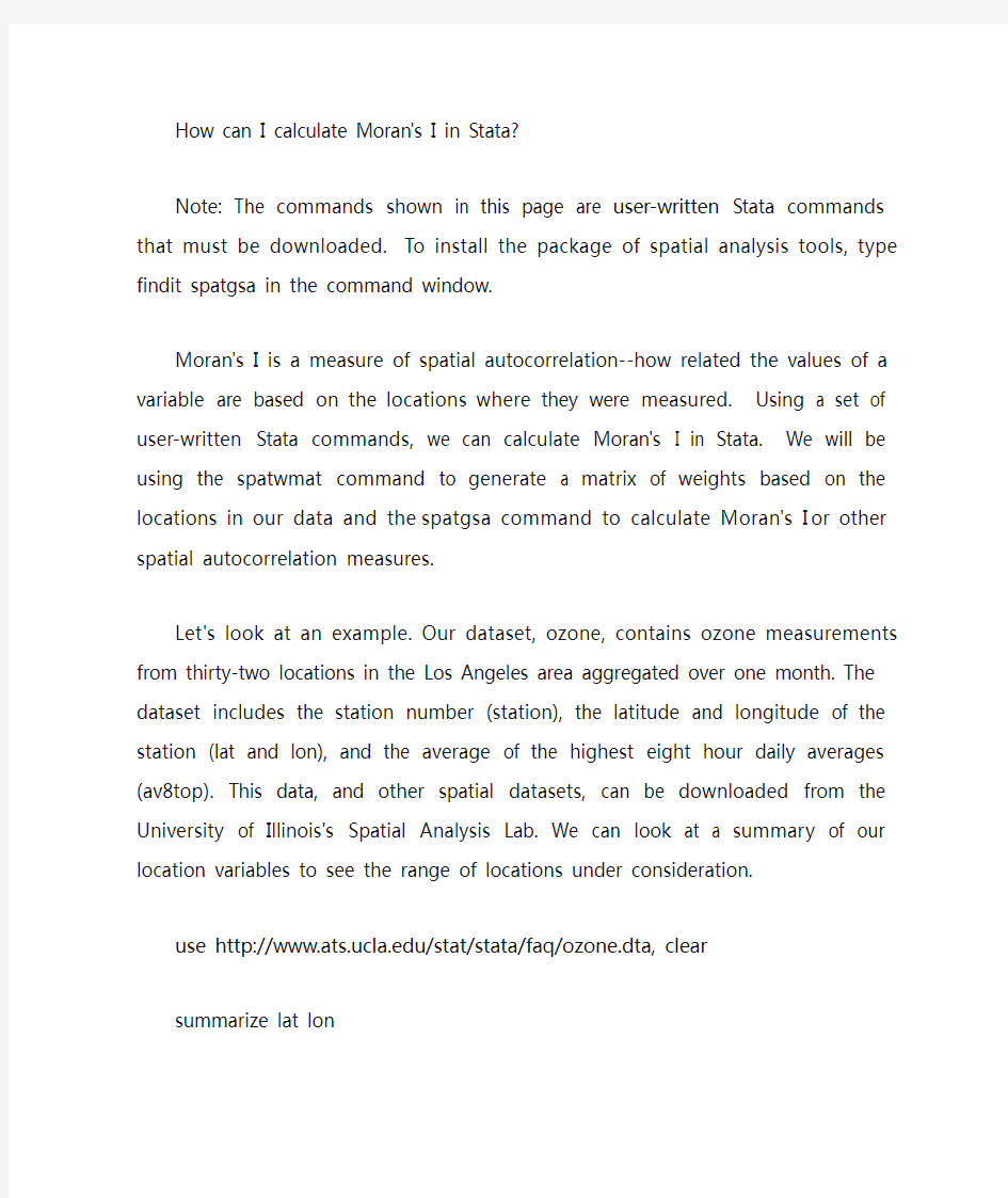
Let's look at an example. Our dataset, ozone, contains ozone measurements from thirty-two locations in the Los Angeles area aggregated over one month. The dataset includes the station number (station), the latitude and longitude of the station (lat and lon), and the average of the highest eight hour daily averages (av8top). This data, and other spatial datasets, can be downloaded from the University of Illinois's Spatial Analysis Lab. We can look at a summary of our location variables to see the range of locations under consideration.
use https://www.360docs.net/doc/169191390.html,/stat/stata/faq/ozone.dta, clear
summarize lat lon
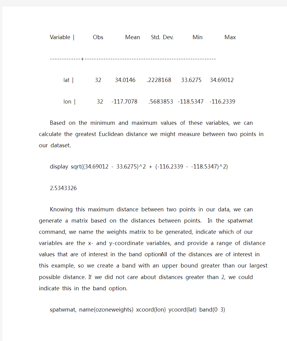
V ariable | Obs Mean Std. Dev. Min Max
-------------+--------------------------------------------------------
lat | 32 34.0146 .2228168 33.6275 34.69012
lon | 32 -117.7078 .5683853 -118.5347 -116.2339
Based on the minimum and maximum values of these variables, we can calculate the greatest Euclidean distance we might measure between two points in our dataset.
display sqrt((34.69012 - 33.6275)^2 + (-116.2339 - -118.5347)^2)
2.5343326
Knowing this maximum distance between two points in our data, we can generate a matrix based on the distances between points. In the spatwmat command, we name the weights matrix to be generated, indicate which of our variables are the x- and y-coordinate variables, and provide a range of distance values that are of interest in the band option. All of the distances are of interest in this example, so we create a band with an upper bound greater than our largest possible distance. If we did not care about distances greater than 2, we could indicate this in the band option.
spatwmat, name(ozoneweights) xcoord(lon) ycoord(lat) band(0 3)
The following matrix has been created:
1. Inverse distance weights matrix ozoneweights
Dimension: 32x32
Distance band: 0 < d <= 3
Friction parameter: 1
Minimum distance: 0.1
1st quartile distance: 0.4
Median distance: 0.6
3rd quartile distance: 1.0
Maximum distance: 2.4
Largest minimum distance: 0.50
Smallest maximum distance: 1.23
As described in the output, the command above generated a matrix with 32 rows and 32 columns because our data includes 32 locations. Each off-diagonal entry [i, j] in the matrix is equal to 1/(distance between point i and point j). Thus, the matrix entries for pairs of points that are close together are higher than for pairs of points that are far apart. If you wish to look at the matrix, you can display it with the matrix list command. With our matrix of weights, we can now calculate Moran's I.
spatgsa av8top, weights(ozoneweights) moran
Measures of global spatial autocorrelation
Weights matrix
--------------------------------------------------------------
Name: ozoneweights
Type: Distance-based (inverse distance)
Distance band: 0.0 < d <= 3.0
Row-standardized: No
--------------------------------------------------------------
Moran's I
--------------------------------------------------------------
V ariables | I E(I) sd(I) z p-value*
--------------------+-----------------------------------------
av8top | 0.248 -0.032 0.036 7.679 0.000
--------------------------------------------------------------
*1-tail test
Based on these results, we can reject the null hypothesis that there is zero spatial autocorrelation present in the variable av8top at alpha = .05.
V ariations
Binary Matrix: If there exists some threshold distance d such that pairs with distances less than d
are neighbors and pairs with distances greater than d are not, you can create a binary neighbors matrix with the spatwmat command (indicating bin and setting band to have an upper bound of d) and use this weights matrix for calculating Moran's I. We could do this for d = .75:
spatwmat, name(ozoneweights) xcoord(lon) ycoord(lat) band(0 .75) bin
The following matrix has been created:
1. Distance-based binary weights matrix ozoneweights
Dimension: 32x32
Distance band: 0 < d <= .75
Friction parameter: 1
Minimum distance: 0.1
1st quartile distance: 0.4
Median distance: 0.6
3rd quartile distance: 1.0
Maximum distance: 2.4
Largest minimum distance: 0.50
Smallest maximum distance: 1.23
spatgsa av8top, weights(ozoneweights) moran
Measures of global spatial autocorrelation
Weights matrix
--------------------------------------------------------------
Name: ozoneweights
Type: Distance-based (binary)
Distance band: 0.0 < d <= 0.75
Row-standardized: No
--------------------------------------------------------------
Moran's I
--------------------------------------------------------------
V ariables | I E(I) sd(I) z p-value*
--------------------+-----------------------------------------
av8top | 0.188 -0.032 0.033 6.762 0.000
--------------------------------------------------------------
*1-tail test
In this example, the binary formulation of distance yields a similar result. We can reject the null hypothesis that there is zero spatial autocorrelation present in the variable av8top at alpha = .05.
Using an existing matrix: If you have calculated a weights matrix according to some other metric than those available in spatwmat and wish to use it in calculating Moran's I, spatwmat allows you to read in a Stata dataset of the required dimensions and format it as a distance matrix that can be used by spatgsa. If altweights.dta is a dataset with 32 columns and 32 rows, it could be converted to a weighted matrix aweights to be used in spatgsa analyzing av8top:
spatwmat using "C:\altweights.dta", name(aweights)
How do I generate a variogram for spatial data in Stata?
When analyzing geospatial data, describing the spatial pattern of a measured variable is of great importance. User written Stata commands allow you to explore such patterns. This page will use the variog and variog2 command. To install this, type findit variog in your command window.
The variog command allows you to calculate and graph a variogram for regularly spaced one-dimensional data. The variog2 command allows you to calculate and graph a variogram for two-dimensional data without constraints on spacing. In both cases, the variogram illustrates how differences in a measured variable Z vary as the distances between the points at which Z is measured increase.
Let's look at an example. Our dataset contains ozone measurements from thirty-two locations in the Los Angeles area aggregated over one month. The dataset includes the station number (station), the latitude and longitude of the station (lat and lon), and the average of the highest eight hour daily averages (av8top). This data, and other spatial datasets, can be downloaded from the GeoDa Center for Geospatial Analysis and Computation.
use https://www.360docs.net/doc/169191390.html,/stat/stata/faq/ozone, clear
clist in 1/5
station av8top lat lon
1. 60 7.225806 34.13583 -117.9236
2. 69 5.899194 34.17611 -118.3153
3. 72
4.052885 33.82361 -118.1875
4. 74 7.181452 34.19944 -118.5347
5. 75
6.076613 34.06694 -11
7.7514
For the sake of an example, let's imagine that instead of specific latitude and longitude locations, the stations are evenly spaced along a single latitude. If we assume the observations are in the order in which the stations appear, we can use the variog command. In the command, we indicate the measured outcome and we will opt for the calculated values to be listed. By default, a plot of the semi-variogram will be generated.
variog av8top, list
+----------------------------------+
| Lag Semi-variance # of pairs |
|----------------------------------|
| 1 2.328506 31 |
| 2 2.615086 30 |
| 3 2.629862 29 |
| 4 2.983584 28 |
| 5 3.415026 27 |
|----------------------------------|
| 6 2.923007 26 |
| 7 4.104437 25 |
| 8 3.378503 24 |
| 9 3.531528 23 |
| 10 4.49281 22 |
|----------------------------------|
| 11 5.22965 21 |
| 12 6.657857 20 |
| 13 6.5462 19 |
| 14 6.126221 18 |
| 15 6.556983 17 |
|----------------------------------|
| 16 6.451519 16 |
+----------------------------------+
Next, let's generate a variogram using the latitude and longitude of the stations. For this, we will use the variog2 command. While the lag distance in variog was assumed to be the distance between each evenly spaced observation, variog2 requires the user to specify the lag distance. Let's look at a summary of our coordinates to get a sense of the distances existing in our data.
summarize lat lon
Variable | Obs Mean Std. Dev. Min Ma x -------------+--------------------------------------------------------
lat | 32 34.0146 .2228168 33.6275 34.69012
lon | 32 -117.7078 .5683853 -118.5347 -116.2339 Based on this, we can calculate the maximum possible distance we might see in our data.
dis sqrt((33.6275 - 34.69012)^2 + (-118.5347 - -116.2339)^2)
2.5343326
As a starting point, we can choose a lag distance of .1 and we can examine distances up to 12 lags apart. We want to choose a lag distance that yields enough pairs in each lag to generate a variance that we trust. We might aim to have at least 15 pairs in each lag.
variog2 av8top lat lon, width(.1) lags(12) list
+----------------------------------+
| Lag Semi-variance # of pairs |
|----------------------------------|
| 1 4.729442 6 |
| 2 1.8984963 31 |
| 3 1.3789778 41 |
| 4 2.7462469 50 |
| 5 4.3899238 49 |
|----------------------------------|
| 6 4.1974818 43 |
| 7 5.2652506 48 |
| 8 7.3351494 41 |
| 9 6.8823236 36 |
| 10 8.0089961 29 |
|----------------------------------|
| 11 6.6957223 29 |
| 12 7.1360346 23 |
+----------------------------------+
We can see that our first lag contains only 6 pairs. We might increase the size of our lags and look at fewer of them.
variog2 av8top lat lon, width(.15) lags(10) list
+----------------------------------+
| Lag Semi-variance # of pairs |
|----------------------------------|
| 1 1.8485044 21 |
| 2 1.8412199 57 |
| 3 3.1204523 74 |
| 4 4.4411303 68 |
| 5 5.8693088 70 |
|----------------------------------|
| 6 7.0979125 55 |
| 7 7.8960334 44 |
| 8 6.5713557 37 |
| 9 4.0710902 23 |
| 10 3.3176015 16 |
+----------------------------------+
In the output, we can see lag distances up to 10*.15 = 1.5, the number of pairs that are this far apart in the dataset, and the semi-variance. As we can see from the plot, the semi-variance increases until the lag distance exceeds .15*7 = 1.05.
STATA最常用命令大全
stata save命令 FileSave As 例1. 表1.为某一降压药临床试验数据,试从键盘输入Stata,并保存为Stata格式文件。 STATA数据库的维护 排序 SORT 变量名1 变量名2 …… 变量更名 rename 原变量名新变量名 STATA数据库的维护 删除变量或记录 drop x1 x2 /* 删除变量x1和x2 drop x1-x5 /* 删除数据库中介于x1和x5间的所有变量(包括x1和x5) drop if x<0 /* 删去x1<0的所有记录 drop in 10/12 /* 删去第10~12个记录 drop if x==. /* 删去x为缺失值的所有记录 drop if x==.|y==. /* 删去x或y之一为缺失值的所有记录 drop if x==.&y==. /* 删去x和y同时为缺失值的所有记录 drop _all /* 删掉数据库中所有变量和数据 STATA的变量赋值 用generate产生新变量 generate 新变量=表达式 generate bh=_n /* 将数据库的内部编号赋给变量bh。 generate group=int((_n-1)/5)+1 /* 按当前数据库的顺序,依次产生5个1,5个2,5个3……。直到数据库结束。 generate block=mod(_n,6) /* 按当前数据库的顺序,依次产生1,2,3,4,5,0。generate y=log(x) if x>0 /* 产生新变量y,其值为所有x>0的对数值log(x),当x<=0时,用缺失值代替。 egen产生新变量 set obs 12 egen a=seq() /*产生1到N的自然数 egen b=seq(),b(3) /*产生一个序列,每个元素重复#次 egen c=seq(),to(4) /*产生多个序列,每个序列从1到# egen d=seq(),f(4)t(6) /*产生多个序列,每个序列从#1到#2 encode 字符变量名,gen(新数值变量名) 作用:将字符型变量转化为数值变量。 STATA数据库的维护 保留变量或记录 keep in 10/20 /* 保留第10~20个记录,其余记录删除 keep x1-x5 /* 保留数据库中介于x1和x5间的所有变量(包括x1和x5),其余变量删除keep if x>0 /* 保留x>0的所有记录,其余记录删除
stata常用命令
用help命令熟悉以下命令的功能: cd:(Change directory)改变stata的工作路径 用法:(cd changes the current working directory to the specified drive and directory.) ●指定全路径:cd e:\ ●指定相对路径(如果当前路径已经指向e:\那么下面命令将达到和上面全路 径命令同样效果): ●cd .. 返回上一级目录 dir:(Display filenames)显示当前目录下的文件信息 用法:(list the names of files in the specified,the names of the commands come from names popular on Unix and Windows,filespec may be any valid Mac, Unix, or Windows file path or file)工作列表文件中指定的名称目录,命令的名称来自名字流行的Unix和Windows文件规范可以是任何有效的Mac,Unix或Windows文件路径或文件。 . dir, w . dir *.dta . dir \mydata\*.dta List:(List values of variables)列出指定变量的取值 用法:(st displays the values of variables. If no varlist is specified, the values of all the variables are displayed)列表显示变量的值。如果没有指定varlist,所有的值显示的变量。list [varlist] [if] [in] [, options] . list in 1/10 . list mpg weight . list mpg weight in 1/20 . list if mpg>20 . list mpg weight if mpg>20 . list mpg weight if mpg>20 in 1/10 Describe:(Describe data in memory or in file)描述内存或者文件中的数 据(样本数、变量类型等信息) 用法:(describe produces a summary of the dataset in memory or of the data stored in a Stata-format dataset. For a compact listing of variable names, use describe, simple.) ●描述内存数据: ●描述文件数据:describe [varlist] using filename [, file_options] Use:(Load Stata dataset)调用数据,打开数据文件(以dta结尾)文 件名+.dta 数据读入stata 用法:(use loads into memory a Stata-format dataset previously saved by save. If filename is specified without an extension, .dta is assumed. If your
[推荐] stata基本操作汇总常用命令
[推荐] Stata基本操作汇总——常用命令 help和search都是查找帮助文件的命令,它们之间的 区别在于help用于查找精确的命令名,而search是模糊查找。 如果你知道某个命令的名字,并且想知道它的具体使用方法,只须在stata的命令行窗口中输入help空格加上这个名字。回车后结果屏幕上就会显示出这个命令的帮助文件的全部 内容。如果你想知道在stata下做某个估计或某种计算,而 不知道具体该如何实现,就需要用search命令了。使用的 方法和help类似,只须把准确的命令名改成某个关键词。回车后结果窗口会给出所有和这个关键词相关的帮助文件名 和链接列表。在列表中寻找最相关的内容,点击后在弹出的查看窗口中会给出相关的帮助文件。耐心寻找,反复实验,通常可以较快地找到你需要的内容.下面该正式处理数据了。我的处理数据经验是最好能用stata的do文件编辑器记下你做过的工作。因为很少有一项实证研究能够一次完成,所以,当你下次继续工作时。能够重复前面的工作是非常重要的。有时因为一些细小的不同,你会发现无法复制原先的结果了。这时如果有记录下以往工作的do文件将把你从地狱带到天堂。因为你不必一遍又一遍地试图重现做过的工作。在stata 窗口上部的工具栏中有个孤立的小按钮,把鼠标放上去会出
现“bring do-file editor to front”,点击它就会出现do文件编 辑器。 为了使do文件能够顺利工作,一般需要编辑do文件的“头”和“尾”。这里给出我使用的“头”和“尾”。capture clear (清空内存中的数据)capture log close (关闭所有 打开的日志文件)set more off (关闭more选项。如果打开该选项,那么结果分屏输出,即一次只输出一屏结果。你按空格键后再输出下一屏,直到全部输完。如果关闭则中间不停,一次全部输出。)set matsize 4000 (设置矩阵的最大阶数。我用的是不是太大了?)cd D: (进入数据所在的盘符和文件夹。和dos的命令行很相似。)log using (文件名).log,replace (打开日志文件,并更新。日志文件将记录下所有文件运行后给出的结果,如果你修改了文件内容,replace选项可以将其更新为最近运行的结果。)use (文件名),clear (打开数据文件。)(文件内容)log close (关闭日志文件。)exit,clear (退出并清空内存中的数据。) 实证工作中往往接触的是原始数据。这些数据没有经过整理,有一些错漏和不统一的地方。比如,对某个变量的缺失观察值,有时会用点,有时会用-9,-99等来表示。回归时如果 使用这些观察,往往得出非常错误的结果。还有,在不同的数据文件中,相同变量有时使用的变量名不同,会给合并数
Stata软件基本操作和数据分析入门
Stata软件基本操作和数据分析入门 第一讲 Stata操作入门 张文彤赵耐青 第一节概况 Stata最初由美国计算机资源中心(Computer Resource Center)研制,现在为Stata公司的产品,其最新版本为7.0版。它操作灵活、简单、易学易用,是一个非常有特色的统计分析软件,现在已越来越受到人们的重视和欢迎,并且和SAS、SPSS一起,被称为新的三大权威统计软件。 Stata最为突出的特点是短小精悍、功能强大,其最新的7.0版整个系统只有10M左右,但已经包含了全部的统计分析、数据管理和绘图等功能,尤其是他的统计分析功能极为全面,比起1G以上大小的SAS系统也毫不逊色。另外,由于Stata在分析时是将数据全部读入内存,在计算全部完成后才和磁盘交换数据,因此运算速度极快。 由于Stata的用户群始终定位于专业统计分析人员,因此他的操作方式也别具一格,在Windows席卷天下的时代,他一直坚持使用命令行/程序操作方式,拒不推出菜单操作系统。但是,Stata的命令语句极为简洁明快,而且在统计分析命令的设置上又非常有条理,它将相同类型的统计模型均归在同一个命令族下,而不同命令族又可以使用相同功能的选项,这使得用户学习时极易上手。更为令人叹服的是,Stata语句在简洁的同时又拥有着极高的灵活性,用户可以充分发挥自己的聪明才智,熟练应用各种技巧,真正做到随心所欲。
除了操作方式简洁外,Stata的用户接口在其他方面也做得非常简洁,数据格式简单,分析结果输出简洁明快,易于阅读,这一切都使得Stata成为非常适合于进行统计教学的统计软件。 Stata的另一个特点是他的许多高级统计模块均是编程人员用其宏语言写成的程序文件(ADO文件),这些文件可以自行修改、添加和下载。用户可随时到Stata网站寻找并下载最新的升级文件。事实上,Stata的这一特点使得他始终处于统计分析方法发展的最前沿,用户几乎总是能很快找到最新统计算法的Stata程序版本,而这也使得Stata自身成了几大统计软件中升级最多、最频繁的一个。 由于以上特点,Stata已经在科研、教育领域得到了广泛应用,WHO的研究人员现在也把Stata作为主要的统计分析工作软件。 第二节 Stata操作入门 一、Stata的界面 图1即为Stata 7.0启动后的界面,除了Windows版本的软件都有的菜单栏、工具栏,状态栏等外,Stata的界面主要是由四个窗口构成,分述如下: 1.结果窗口:位于界面右上部,软件运行中的所有信息,如所执行的命令、执行结果和出错信息等均在这里列出。窗口中会使用不同的颜色区分不同的文本,如白色表示命令,红色表示错误信息。 2.命令窗口:位于结果窗口下方,相当于DOS软件中的命令行,此处用于键入需要执行的命令,回车后即开始执行,相应的结果则会在结果窗口中显示出来。
STATA命令应用及详细解释(汇总情况)
STATA命令应用及详细解释(汇总) 调整变量格式: format x1 .3f ——将x1的列宽固定为10,小数点后取三位 format x1 .3g ——将x1的列宽固定为10,有效数字取三位 format x1 .3e ——将x1的列宽固定为10,采用科学计数法 format x1 .3fc ——将x1的列宽固定为10,小数点后取三位,加入千分位分隔符 format x1 .3gc ——将x1的列宽固定为10,有效数字取三位,加入千分位分隔符 format x1 %-10.3gc ——将x1的列宽固定为10,有效数字取三位,加入千分位分隔符,加入“-”表示左对齐 合并数据: use "C:\Documents and Settings\xks\桌面\2006.dta", clear merge using "C:\Documents and Settings\xks\桌面\1999.dta" ——将1999和2006的数据按照样本(observation)排列的自然顺序合并起来 use "C:\Documents and Settings\xks\桌面\2006.dta", clear merge id using "C:\Documents and Settings\xks\桌面
\1999.dta" ,unique sort ——将1999和2006的数据按照唯一的(unique)变量 id来合并,在合并时对id进行排序(sort) 建议采用第一种方法。 对样本进行随机筛选: sample 50 在观测案例中随机选取50%的样本,其余删除 sample 50,count 在观测案例中随机选取50个样本,其余删除 查看与编辑数据: browse x1 x2 if x3>3 (按所列变量与条件打开数据查看器)edit x1 x2 if x3>3 (按所列变量与条件打开数据编辑器)数据合并(merge)与扩展(append) merge表示样本量不变,但增加了一些新变量;append表示样本总量增加了,但变量数目不变。 one-to-one merge: 数据源自stata tutorial中的exampw1和exampw2 第一步:将exampw1按v001~v003这三个编码排序,并建立临时数据库tempw1 clear use "t:\statatut\exampw1.dta" su
常用到的stata命令
常用到的sta命令 闲话不说了。help和search都是查找帮助文件的命令,它们之间的区别在于help用于查找精确的命令名,而search是模糊查找。如果你知道某个命令的名字,并且想知道它的具体使用方法,只须在sta的命令行窗口中输入help空格加上这个名字。回车后结果屏幕上就会显示出这个命令的帮助文件的全部内容。如果你想知道在sta下做某个估计或某种计算,而不知道具体该如何实现,就需要用search命令了。使用的方法和help类似,只须把准确的命令名改成某个关键词。回车后结果窗口会给出所有和这个关键词相关的帮助文件名和链接列表。在列表中寻找最相关的内容,点击后在弹出的查看窗口中会给出相关的帮助文件。耐心寻找,反复实验,通常可以较快地找到你需要的内容。 下面该正式处理数据了。我的处理数据经验是最好能用sta的do文件编辑器记下你做过的工作。因为很少有一项实证研究能够一次完成,所以,当你下次继续工作时。能够重复前面的工作是非常重要的。有时因为一些细小的不同,你会发现无法复制原先的结果了。这时如果有记录下以往工作的do文件将把你从地狱带到天堂。因为你不必一遍又一遍地试图重现做过的工作。在sta窗口上部的工具栏中有个孤立的小按钮,把鼠标放上去会出现“bring do-file editor to front”,点击它就会出现do文件编辑器。 为了使do文件能够顺利工作,一般需要编辑do文件的“头”和“尾”。这里给出我使用的“头”和“尾”。 /*(标签。简单记下文件的使命。)*/ capture clear(清空内存中的数据) capture log close(关闭所有打开的日志文件) set mem 128m(设置用于sta使用的内存容量) set more off(关闭more选项。如果打开该选项,那么结果分屏输出,即一次只输出一屏结果。你按空格键后再输出下一屏,直到全部输完。如果关闭则中间不停,一次全部输出。) set matsize4000(设置矩阵的最大阶数。我用的是不是太大了?)
Stata统计分析命令
Stata统计分析常用命令汇总 一、winsorize极端值处理 范围:一般在1%和99%分位做极端值处理,对于小于1%的数用1%的值赋值,对于大于99%的数用99%的值赋值。 1、Stata中的单变量极端值处理: stata 11.0,在命令窗口输入“findit winsor”后,系统弹出一个窗口,安装winsor模块 安装好模块之后,就可以调用winsor命令,命令格式:winsor var1, gen(new var) p(0.01) 或者在命令窗口中输入:ssc install winsor安装winsor命令。winsor命令不能进行批量处理。 2、批量进行winsorize极端值处理: 打开链接:https://www.360docs.net/doc/169191390.html,/judson.caskey/data.html,找到winsorizeJ,点击右键,另存为到stata中的ado/plus/目录下即可。命令格式:winsorizeJ var1var2var3,suffix(w)即可,这样会生成三个新变量,var1w var2w var3w,而且默认的是上下1%winsorize。如果要修改分位点,则写成如下格式:winsorizeJ var 1 var2 var3,suffix(w) cuts(5 95)。 3、Excel中的极端值处理:(略) winsor2 命令使用说明 简介:winsor2 winsorize or trim (if trim option is specified) the variables in varlist at particular percentiles specified by option cuts(# #). In defult, new variables will be generated with a suffix "_w" or "_tr", which can be changed by specifying suffix() option. The replace option replaces the variables with their winsorized or trimmed ones. 相比于winsor命令的改进: (1) 可以批量处理多个变量; (2) 不仅可以winsor,也可以trimming; (3) 附加了by() 选项,可以分组winsor 或trimming; (4) 增加了replace 选项,可以不必生成新变量,直接替换原变量。 范例: *- winsor at (p1 p99), get new variable "wage_w" . sysuse nlsw88, clear . winsor2 wage *- left-trimming at 2th percentile . winsor2 wage, cuts(2 100) trim *- winsor variables by (industry south), overwrite the old variables . winsor2 wage hours, replace by(industry south) 使用方法: 1. 请将winsor 2.ado 和winsor2.sthlp 放置于stata12\ado\base\w 文件夹下; 2. 输入help winsor2 可以查看帮助文件;
STATA统计分析入门
STATA统计分析入门 STATA统计软件包是目前世界上最著名的统计软件之一,与SAS、SPSS一起被并称为三大权威软件。它广泛的应用于经济、教育、人口、政治学、社会学、医学、药学、工矿、农林等学科领域,同时具有数据管理软件、统计分析软件、绘图软件、矩阵计算软件和程序语言的特点,几乎可以完成全部复杂的统计分析工作。其功能非常强大且操作简单、使用灵活、易学易用、运行速度极快,在许多方面别具一格。 STATA最为突出的特点是短小精悍、功能强大,整个系统一般在200M左右,但是已经包含了全部的统计分析。数据管理和绘图等功能,尤其是它的统计分析功能极为全面,比起1G以上大小的SAS系统也毫不逊色。而且STATA在分析时是将数据全部读入内存,在计算全部完成后才和磁盘交换数据,因此运算速度极快。STATA的命令语句也极为简洁明快,而且在统计分析命令的设置上又非常有条理,它将相同类型的统计模型均归在同一个命令族下,而不同命令族又可以使用相同功能的选项,这使得用户学习时极易上手。STATA语句在简洁的同时又拥有着极高的灵活性,用户可以充分发挥自己的聪明才智,熟练应用各种技巧,真正做到随心所欲。 STATA的另一个特点是他的许多高级统计模块均是编程人员用宏语言写成的程 序文件(ADO文件),这些文件可以自行修改、添加和下载。用户可随时到STATA 网站寻找并下载最新的升级文件。 课程简介: 该课程主要是为大家介绍STATA的基本用法和简单的统计分析。 课程大纲: 第一课:STATA简介 介绍STATA基本情况(统计编程及作图功能),软件窗口界面及基本数据处理的操作方法。 第二课:STATA中的图形制作 介绍图形制作的基本命令和一些基本图形的绘制(直方图、散点图、箱线图、饼图等) 第三课:假设检验与方差分析ANOVA STATA下单双因素方差分析的操作,及假设检验 第四课:简单与多元回归 介绍大小样本下的最小二乘法与多元线性回归,介绍如何用STATA做回归诊断 课程基础: 简单的英文基础,因为STATA是英文版的
(完整)stata命令总结,推荐文档
stata11常用命令 注:JB统计量对应的p大于0.05,则表明非正态,这点跟sktest和swilk 检验刚好相反; dta为数据文件; gph为图文件; do为程序文件; 注意stata要区别大小写; 不得用作用户变量名: _all _n _N _skip _b _coef _cons _pi _pred _rc _weight double float long int in if using with 命令: 读入数据一种方式 input x y 1 4 2 5.5 3 6.2 4 7.7 5 8.5 end su/summarise/sum x 或 su/summarise/sum x,d 对分组的描述: sort group by group:su x %%%%% tabstat economy,stats(max) %返回变量economy的最大值 %%stats括号里可以是:mean,count(非缺失观测值个数),sum(总和),max,min,range, %% sd,var,cv(变易系数=标准差/均值),skewness,kurtosis,median,p1(1%分位 %% 数,类似地有p10, p25, p50, p75, p95, p99),iqr(interquantile range = p75 – p25) _all %描述全部 _N 数据库中观察值的总个数。 _n 当前观察值的位置。 _pi 圆周率π的数值。 list gen/generate %产生数列 egen wagemax=max(wage) clear use by(分组变量)
如何运用Stata完成统计数据汇总工作论文.doc
本加总在一起,合并后样本变量数目不变,样本数增加,也就是数据文件变长了。最常见的纵向合并情况是对一项调查在不同地区或者不同时间得来的数据进行合并。Stata 纵向合并数据文件的命令为“append”.比如,我们将调查得到的包含北京市调查数据的数据文件“bj.dta”和包含天津市调查数据的数据文件“tj.dta”纵向合并的Stata命 令为: use bj,clear append using tj 需要注意的是,在纵向合并两个数据文件前,两个文件中相同变量的变量名要一致,否则将会被当成两个变量处理,并产生无用的缺失值。同时,相同变量的变量类型要一致。 汇总问卷调查结果 问卷调查时效性较强,调查结果容易量化,便于统计处理与分析,是常用的统计调查方法。问卷调查结果用Stata 进行汇总非常方便,使用“tabulate”命令,可方便的生成列联表,根据变量的频数分布可以得到问卷回答情况的汇总结果。比如,对10000个样本企业开展问卷调查,涉及10 个问题,分别为:
WT1,WT2, ……,WT10(每个问题的答案均为A、B、C、D 四个选项)。汇总问题WT1 的回答情况时,只需输入命令:tabulateWT1,即可得到WT1 样本回答情况的频数(Freq)、百分比(Percent)及累计百分比(Cum)指标(Stata 输出结果见表1)。从Freq 输出结果可见,样本企业对WT1 的回答情况为:选择答案A、B、C、D 的企业数量分别为1000、3000、4000 和2000 个。Percent结果给出了选择答案1、2、3、4 的比重分别为10%,30%、40% 和20%. 同时,“tabulate”命令还可以生成2 维列联表,比如,需要对问题WT1 做分省回答结果的汇总时,只需对省代码(sf)和WT1 执行“tabulate”汇总。Stata 命令为:tabulate sf WT1,即可输出表 2 格式的汇总结果{ 假设调查只涉及北京市(代码11)、天津市(代码12)、河北省(代码13)}. 类似的,可以对每一个问题的调查结果分行业、分登记注册类型、分控股情况等做交叉分组汇总。 汇总生产经营情况调查结果 现行的统计报表制度更多的是对调查单位的生产经营情况开展年度、季度或者是月度调查。日常的数据汇总工作更多的是对生产经营指标做各种交叉分组汇总。 与问卷调查结果不同,生产经营情况的调查结果需要对调查指标数据加总或者通过计算生成新的指标,因此,我们首先要生成新的变量,来记录相应指标的汇总结果。Stata 生成新变量的命令为“generate”及其扩展命令“egen”.“generate”用来生
stata命令大全
调整变量格式: format x1 %10.3f ——将x1的列宽固定为10,小数点后取三位 format x1 %10.3g ——将x1的列宽固定为10,有效数字取三位 format x1 %10.3e ——将x1的列宽固定为10,采用科学计数法 format x1 %10.3fc ——将x1的列宽固定为10,小数点后取三位,加入千分位分隔符 format x1 %10.3gc ——将x1的列宽固定为10,有效数字取三位,加入千分位分隔符 format x1 %-10.3gc ——将x1的列宽固定为10,有效数字取三位,加入千分位分隔符,加入“-”表示左对齐 合并数据: use "C:\Documents and Settings\xks\桌面\2006.dta", clear merge using "C:\Documents and Settings\xks\桌面\1999.dta" ——将1999和2006的数据按照样本(observation)排列的自然顺序合并起来 use "C:\Documents and Settings\xks\桌面\2006.dta", clear merge id using "C:\Documents and Settings\xks\桌面\1999.dta" ,unique sort ——将1999和2006的数据按照唯一的(unique)变量id来合并,在合并时对id进行排序(sort)建议采用第一种方法。 对样本进行随机筛选: sample 50 在观测案例中随机选取50%的样本,其余删除 sample 50,count 在观测案例中随机选取50个样本,其余删除 查看与编辑数据: browse x1 x2 if x3>3 (按所列变量与条件打开数据查看器) edit x1 x2 if x3>3 (按所列变量与条件打开数据编辑器) 数据合并(merge)与扩展(append) merge表示样本量不变,但增加了一些新变量;append表示样本总量增加了,但变量数目不变。one-to-one merge: 数据源自stata tutorial中的exampw1和exampw2 第一步:将exampw1按v001~v003这三个编码排序,并建立临时数据库tempw1 clear use "t:\statatut\exampw1.dta" su ——summarize的简写 sort v001 v002 v003 save tempw1 第二步:对exampw2做同样的处理 clear use "t:\statatut\exampw2.dta" su sort v001 v002 v003 save tempw2 第三步:使用tempw1数据库,将其与tempw2合并: clear use tempw1 merge v001 v002 v003 using tempw2
运用Stata做计量经济学
运用Stata做计量经济学 运用Stata建模的7步骤: 1、准备工作;目录、日志、读入数据、熟悉数据、时间变量、more、……; 2、探索数据:数据变换、描述统计量、相关系数、趋势图、散点图、……; 3、建立模型:regress、经济理论检验、实际经济问题要求、统计学检验、计量经济学检验:R2,T,t,残差; 4、诊断模型:异方差、序列相关、多重共线性、随机解释变量问题、……; 5、修正模型:WLS、GLS、工具变量法(ivregress),……; 6、应用模型:置信区间、预测、结构分析、边际分析、弹性分析、常用模型回归系数的意义、……; 7、整理:关闭日志、生成do文件备用 1、准备工作 让STATA处于初始状态,清除所有使用过的痕迹clear 指明版本号version11 设定并进入工作文件夹:cd D:\ (设定路径,将数据、程序和输出结果文件均存入该文件夹) 关闭以前的日志capture log close 建立日志:log using , replace 设定内存:set mem 20m
关闭more:set more off 读入数据:use .dta, clear 认识变量:describe 建立时间变量:tsset 2、用描述统计方法探索数据特征 必要的数据转换:gen、replace、……; 描述统计量:summarize, detail 相关系数矩阵:corr/pwcorr 散点图和拟合直线图:scatter y x || lfit y x 矩阵散点图:graph matrix y x1 x2 x3,half 线性趋势图:line y x 3、建立模型 OLS建立模型:regress y x1 x2 x3; 由方差分析表并用F和R2检验模型整体显著性; 依据p值对各系数进行t检验,一次只能剔出一个最不显著的变量,直到不包含不显著的变量; 估计参数,判别变量的相对重要性; 构造和估计约束模型,用以检验经济理论
stata常用命令
面板数据估计 首先对面板数据进行声明: 前面是截面单元,后面是时间标识: tsset company year tsset industry year 产生新的变量:gen newvar=human*lnrd 产生滞后变量Gen fiscal(2)=L2.fiscal 产生差分变量Gen fiscal(D)=D.fiscal 描述性统计: xtdes :对Panel Data截面个数、时间跨度的整体描述 Xtsum:分组内、组间和样本整体计算各个变量的基本统计量 xttab 采用列表的方式显示某个变量的分布 Stata中用于估计面板模型的主要命令:xtreg xtreg depvar [varlist] [if exp] , model_type [level(#) ] Model type 模型 be Between-effects estimator fe Fixed-effects estimator re GLS Random-effects estimator pa GEE population-averaged estimator mle Maximum-likelihood Random-effects estimator 主要估计方法: xtreg: Fixed-, between- and random-effects, and population-averaged linear models xtregar:Fixed- and random-effects linear models with an AR(1) disturbance xtpcse :OLS or Prais-Winsten models with panel-corrected standard errors xtrchh :Hildreth-Houck random coefficients models
stata常用命令
stata常用命令 stata save命令 FileSave As 例1. 表1.为某一降压药临床试验数据,试从键盘输入Stata,并保存为Stata格式文件。STATA数据库的维护 排序 SORT 变量名1 变量名2 …… 变量更名 rename 原变量名新变量名 STATA数据库的维护 删除变量或记录 drop x1 x2 /* 删除变量x1和x2 drop x1-x5 /* 删除数据库中介于x1和x5间的所有变量(包括x1和x5) drop if x<0 /* 删去x1<0的所有记录 drop in 10/12 /* 删去第10~12个记录 drop if x==. /* 删去x为缺失值的所有记录 drop if x==.|y==. /* 删去x或y之一为缺失值的所有记录 drop if x==.&y==. /* 删去x和y同时为缺失值的所有记录 drop _all /* 删掉数据库中所有变量和数据 STATA的变量赋值 用generate产生新变量 generate 新变量=表达式 generate bh=_n /* 将数据库的内部编号赋给变量bh。 generate group=int((_n-1)/5)+1 /* 按当前数据库的顺序,依次产生5个1,5个2,5个3……。直到数据库结束。 generate block=mod(_n,6) /* 按当前数据库的顺序,依次产生1,2,3,4,5,0。generate y=log(x) if x>0 /* 产生新变量y,其值为所有x>0的对数值log(x),当x<=0时,用缺失值代替。 egen产生新变量 set obs 12 egen a=seq() /*产生1到N的自然数 egen b=seq(),b(3) /*产生一个序列,每个元素重复#次 egen c=seq(),to(4) /*产生多个序列,每个序列从1到# egen d=seq(),f(4)t(6) /*产生多个序列,每个序列从#1到#2
常用stata命令-好用
我常用到的stata命令 最重要的两个命令莫过于help和search了。即使是经常使用stata的人也很难,也没必要记住常用命令的每一个细节,更不用说那些不常用到的了。所以,在遇到困难又没有免费专家咨询时,使用stata自带的帮助文件就是最佳选择。stata的帮助文件十分详尽,面面俱到,这既是好处也是麻烦。当你看到长长的帮助文件时,是不是对迅速找到相关信息感到没有信心? 闲话不说了。help和search都是查找帮助文件的命令,它们之间的区别在于help用于查找精确的命令名,而search是模糊查找。如果你知道某个命令的名字,并且想知道它的具体使用方法,只须在stata的命令行窗口中输入help空格加上这个名字。回车后结果屏幕上就会显示出这个命令的帮助文件的全部内容。如果你想知道在stata下做某个估计或某种计算,而不知道具体该如何实现,就需要用search命令了。使用的方法和help类似,只须把准确的命令名改成某个关键词。回车后结果窗口会给出所有和这个关键词相关的帮助文件名和链接列表。在列表中寻找最相关的内容,点击后在弹出的查看窗口中会给出相关的帮助文件。耐心寻找,反复实验,通常可以较快地找到你需要的内容。 下面该正式处理数据了。我的处理数据经验是最好能用stata的do文件编辑器记下你做过的工作。因为很少有一项实证研究能够一次完成,所以,当你下次继续工作时。能够重复前面的工作是非常重要的。有时因为一些细小的不同,你会发现无法复制原先的结果了。这时如果有记录下以往工作的do文件将把你从地狱带到天堂。因为你不必一遍又一遍地试图重现做过的工作。在stata窗口上部的工具栏中有个孤立的小按钮,把鼠标放上去会出现“bring do-file editor to front”,点击它就会出现do文件编辑器。 为了使do文件能够顺利工作,一般需要编辑do文件的“头”和“尾”。这里给出我使用的“头”和“尾”。 /*(标签。简单记下文件的使命。)*/ capture clear (清空内存中的数据) capture log close (关闭所有打开的日志文件) set mem 128m (设置用于stata使用的内存容量) set more off (关闭more选项。如果打开该选项,那么结果分屏输出,即一次只输出一屏结果。你按空格键后再输出下一屏,直到全部输完。如果关闭则中间不停,一次全部输出。)set matsize 4000 (设置矩阵的最大阶数。我用的是不是太大了?) cd D: (进入数据所在的盘符和文件夹。和dos的命令行很相似。) log using (文件名).log,replace (打开日志文件,并更新。日志文件将记录下所有文件运行后给出的结果,如果你修改了文件内容,replace选项可以将其更新为最近运行的结果。) use (文件名),clear (打开数据文件。) (文件内容)
stata常用命令
调整变量格式: format x1 % ——将x1的列宽固定为10,小数点后取三位 format x1 % ——将x1的列宽固定为10,有效数字取三位 format x1 % ——将x1的列宽固定为10,采用科学计数法 format x1 % ——将x1的列宽固定为10,小数点后取三位,加入千分位分隔符 format x1 % ——将x1的列宽固定为10,有效数字取三位,加入千分位分隔符 format x1 % ——将x1的列宽固定为10,有效数字取三位,加入千分位分隔符,加入“-”表示左对齐合并数据: use "C:\Documents and Settings\xks\桌面\", clear merge using "C:\Documents and Settings\xks\桌面\" ——将1999和2006的数据按照样本(observation)排列的自然顺序合并起来 use "C:\Documents and Settings\xks\桌面\", clear merge id using "C:\Documents and Settings\xks\桌面\" ,unique sort ——将1999和2006的数据按照唯一的(unique)变量id来合并,在合并时对id进行排序(sort)建议采用第一种方法。 对样本进行随机筛选: sample 50 在观测案例中随机选取50%的样本,其余删除 sample 50,count 在观测案例中随机选取50个样本,其余删除 查看与编辑数据: browse x1 x2 if x3>3 (按所列变量与条件打开数据查看器) edit x1 x2 if x3>3 (按所列变量与条件打开数据编辑器) 数据合并(merge)与扩展(append) merge表示样本量不变,但增加了一些新变量;append表示样本总量增加了,但变量数目不变。one-to-one merge: 数据源自stata tutorial中的exampw1和exampw2 第一步:将exampw1按v001~v003这三个编码排序,并建立临时数据库tempw1 clear use "t:\statatut\" su ——summarize的简写 sort v001 v002 v003 save tempw1 第二步:对exampw2做同样的处理 clear use "t:\statatut\" su sort v001 v002 v003 save tempw2 第三步:使用tempw1数据库,将其与tempw2合并: clear use tempw1 merge v001 v002 v003 using tempw2 第四步:查看合并后的数据状况:
Stata命令大全-面板数据计量分析与软件实现
Stata命令大全面板数据计量分析与软件实现 说明:以下do文件相当一部分内容来自于中山大学连玉君STATA教程,感谢他的贡献。本人做了一定的修改与筛选。 *----------面板数据模型 * 1.静态面板模型:FE 和RE * 2.模型选择:FE vs POLS, RE vs POLS, FE vs RE (pols混合最小二乘估计) * 3.异方差、序列相关和截面相关检验 * 4.动态面板模型(DID-GMM,SYS-GMM) * 5.面板随机前沿模型 * 6.面板协整分析(FMOLS,DOLS) *** 说明:1-5均用STATA软件实现, 6用GAUSS软件实现。 * 生产效率分析(尤其指TFP):数据包络分析(DEA)与随机前沿分析(SFA) *** 说明:DEA由DEAP2.1软件实现,SFA由Frontier4.1实现,尤其后者,侧重于比较C-D与Translog生产函数,一步法与两步法的区别。常应用于地区经济差异、FDI 溢出效应(Spillovers Effect)、工业行业效率状况等。 * 空间计量分析:SLM模型与SEM模型 *说明:STATA与Matlab结合使用。常应用于空间溢出效应(R&D)、财政分权、地方政府公共行为等。 * --------------------------------- * --------一、常用的数据处理与作图----------- * --------------------------------- * 指定面板格式 xtset id year (id为截面名称,year为时间名称) xtdes /*数据特征*/ xtsum logy h /*数据统计特征*/ sum logy h /*数据统计特征*/ *添加标签或更改变量名 label var h "人力资本"
Stata教程:描述性统计命令与输出结果说明
本节STATA命令摘要 by 分组变量:]summarize变量名1变量名2… 变量名m[,detail] ci变量名1变量名2… 变量名m[,level(#)binomial poissonexposure(varname)by(分组变量)] cii 样本量 均数 标准差[,level(#)] tab1变量名[,generate(变量名)] · 资料特征描述(均数,中位数,离散程度) 例:某地测定克山病患者与克山病健康人的血磷测定值如下表(数据摘自四川医学院主编的卫生统计学,1978出版,p21): 患者 2.6 3.24 3.73 3.73 4.32 4.73 5.18 5.58 5.78 6.40 6.53 健康人 1.67 1.98 1.98 2.33 2.34 2.50 3.60 3.73 4.14 4.17 4.57 4.82 5.78 并假定这些数据已以STATA格式存入ex2.dta文件中,其中变量x1为患者的血磷测定值数据,变量x2为健康人的血磷测定值数据。上述数据也可以用变量x表示血磷测
定值,分组变量group=0表示患者组和group=1表示健康组(如:患者组中第一个数据为2.6,则x=2.6,group=0;又如:健康组中第三个数据为1.98,则x为1.98以及group为1),并假定这些数据已以STATA格式存入ex2a.dta文件中。 计算资料均数,标准差命令summarize,以述资料为例: useex2,clear summarizex1x2 结果: 变量 样本数 均数 标准差 最小值 最大值 Variable| Obs Mean Std.Dev. Min Max ---------+ x1| 11 4.710909 1.302977 2.6 6.53 x2| 13 3.354615 1.304368 1.67 5.78 即:本例中急性克山病患者组的样本数为11,血磷测定值均数为4.711(mg%),相应的标准差为1.303,最小值为2.6以及最大值为6.53;健康组的样本量为13,血磷测定值均数为3.3546,相应的标准差为1.3044,最小值为1.67以及最大值为5.78。 计算资料均数,标准差,中位数,低四分位数和高四分位数的命令summarize 以及子命令detail,仍以述资料为例: use ex2,clear summarizex1x2,detail 结果: x1 Percentiles Smallest(最小值) 1%