北大暑期课程《回归分析》(Linear-Regression-Analysis)讲义1复习过程
北大暑期课程《回归分析》(Linear-Regression-Analysis)讲义3
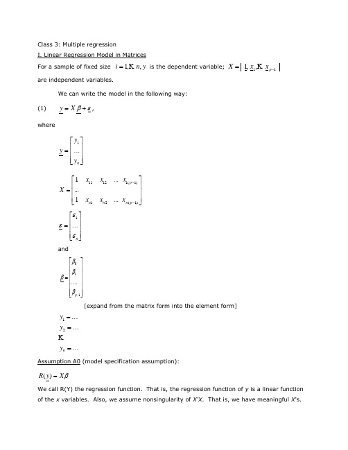
Class 3: Multiple regressionI. Linear Regression Model in Matrices For a sample of fixed size y n i,,1 is the dependent variable; 11,,1 p x x Xare independent variables. We can write the model in the following way:(1) X y ,wheren y y y (1))1()1(1211211...1......1p n p n n x x x x x x Xn (1)and110....p[expand from the matrix form into the element form]Assumption A0 (model specification assumption):X y R )(We call R(Y) the regression function. That is, the regression function of y is a linear function of the x variables. Also, we assume nonsingularity of X'X . That is, we have meaningful X 's..........21 n y y yII. Least Squares Estimator in Matrices Pre-multiply (1) by X ' (2),'''1 X X X y X pAssumption A1 (orthogonality assumption): we assume that is uncorrelated with each and every vector in X . That is,(3).0)(0),(0)(0),(0)(0),(0)(112111 p p x E x Cov x E x Cov x E x Cov ESample analog of expectation operator is n1. Thus, we have(4)01010101)1(21 i p i i i i i i x nx n x n n That is, there are a total of p restriction conditions, necessary for solving p linear equations to identify p parameters. In matrix format, this is equivalent to:(5).][or,][1o X o X nSubstitute (5) into (2), we have (6))()(X X y XThe LS estimator is then:(7),)(1y X X X bwhich is the same as the least squares estimator. Note: A1 assumption is needed for avoiding biases. III. Properties of the LS Estimator For the mode X y ,A1]using result, [important ][)(][)(])[(])[()]()[(])[()()(1111111o X E X X E X X X X X X X E X X X X E X X X X E y X X X E b E y X X X bthat is, b is unbiased.V (b ) is a symmetric matrix, called variance and covariance matrix of b .)(......)...(),(...),()()(1110100p b V b V b b Cov b b Cov b V b V 1111111)(][)()on al (condition ])[()])()[()]()[(])[()( X X X V X X X X X X X V O X X X X X X X V X X X X V y X X X V b V(after assuming I V 2][ non-serial correlation and homoscedasticity)21)( X X [important result, using A2][blackboard ]22001. Assumption A2 (iid assumption): independent and identically distributed errors. Two implications:1. Independent disturbances, j i E j i ,0),(Obtaining neat v (b ).2. Homoscedasticity, j i v E i j i ,)()(2Obtaining neat v (b ).I V 2)( , scalar matrix.IV. Fitted Values and Residualsy H y X X X X b X y 1)(ˆ X X X X H n n 1)(is called H matrix, or hat matrix. H is an idempotent matrix:H HHFor residuals:y H I y H y yy e )(ˆ (I-H ) is also an idempotent matrix.V. Estimation of the Residual Variance A. Sample Analog (8))()]([)(222i i i i E E E Vis unknown but can be estimated by e , where e is residual. Some of you may have noticedthat I have intentionally distinguished from e . is called disturbance, and e is called residual. Residual is defined by the difference between observed and predicted values.The sample analog of (8) is2)1()1(2211022)]([1)ˆ(11 p i p i i i i i i x b x b x b b y ny y n e nIn matrix:e e e i 2The sample analog is thenn e e /B. Degrees of FreedomAs a general rule, the correct degrees of freedom equals the number of totalobservations minus the number of parameters used in estimation.In multiple regression, there are p parameters to be estimated. Therefore, theremaining degrees of freedom for estimating disturbance variance is n-p . C. MSE as the EstimatorMSE is the unbiased estimator. It is unbiased because it corrects for the loss ofdegrees of freedom in estimating the parameters.ee p n MSE e pn MSE i112D. Statistical InferencesNow that we have point estimates (b ) and the variance-covariance matrix of b . But wecannot do formal statistical tests yet. The question, then, is how to make statistical inferences, such as testing hypotheses and constructing confidence intervals. Well, the only remaining thing we need is the ability to use some tests, say t , Z , or F tests.Statistical theory tells us that we can conduct such tests if e is not only iid, but iid in anormal distribution. That is, we assumeAssumption A3 (normality assumption): i is distributed as ),0(2NWith this assumption, we can look up tables for small samples.However, A3 is not necessary for large samples. For large samples, central limit theoryassures that we can still make the same statistical inferences based on t, z , or F tests if the sample is large enough.A Summary of Assumptions for the LS Estimator 1. A0: Specification assumptionX X y )|(EIncluding nonsingularity of X X .Meaningful X 's.With A0, we can computey X X X b 1)(2. A1:orthoganality assumption0)(k x E , for k = 0, .... p-1, x 0 = 1.Meaning: 0)( E is needed for the identification of 0 .All other column vectors in X are orthogonal with respect to .A1 is needed for avoiding biases. With A1, b is unbiased and consistent estimator of . Unbiasedness means that)(b EConsistency: n b as .For large samples, consistency is the most important criterion for evaluating estimators.3. A2. iid independent and identically distributed errors. Two implications:1. Independent disturbances, j i Cov j i ,0),(Obtaining neat v(b).2. Homoscedasticity, j i v Cov i j i ,)(),(2Obtaining neat v(b).I V 2)( , scalar matrix.With A2, b is an efficient estimator.Efficiency: an efficient estimator has the smallest sampling variance among all unbiased estimators. That is),ˆ()(Var somehow b Var whereˆ denotes any unbiased estimator. Roughly, for efficient estimators, imprecision [i.e., SD(b )] decreases by the inverse of the square root of n . That is, if you wish to increase precision by 10 times, (i.e., reduce S.E. by a factor of ten), you would need to increase the sample size by 100 times.A1 + A2 make OLS a BLUE estimator, where BLUE means the best, linear, unbiased estimator. That is, no other unbiased linear estimator has a smaller sampling variance than b .This result is called "Gauss-Markov theorem."4. A3. Normality, i is distributed as ),0(2NInferences: looking up tables for small samples.A1 + A2 + A3 make OLS a maximum likelihood (ML) estimator. Like all other ML estimators, OLS in this case is BUE (best unbiased estimator). That is, no other unbiased estimator can have a smaller sampling variance than OLS.Note that ML is always the most efficient estimator among all unbiased estimators. The cost of ML is really the requirement of we know the true parametric distribution of the residual. If you can afford the assumption, ML is always the best. Very often, we don't make the assumption because we don't know the parametric family of the disturbance. In general, the following tradeoff is true:More information == more efficiency. Less assumption == less efficiency.It is not correct to call certain models OLS models and other ML models. Theoretically, a same model can be estimated by OLS or ML. Model specification is different from estimation procedure.VI. ML for linear model under normality assumption (A1+A2+A3) , i :i :d N(0, 2), i = 1, … nObservations y i are independently distributed as y i ~ N(x i ’ 2); i = 1, … nUnder the normal errors assumption, the joint pdf of y’s isL = f (y 1…y n | 2) = ∏ f (y i | 2)= (2π 2)-n/2 exp{-(2 2)-1∑(y i - x i ’ }Log transformation is a monotone transformation. Maximizing L is equivalent to maximizing logL below:l = logL = (-n/2) log(2π 2) - (2 2)-1 ∑(y i - x i ’It is easy to see that what maximizes l (Maximum Likelihood Estimator) is the same as the LS estimator.。
定量分析实验室项目课程介绍
定量分析实验室项目课程介绍
1、回归分析(Linear Regression Analysis):
教师:Yu Xie(谢宇),美国密歇根大学社会学系教授。
时间:2007年7月16日至8月10日
课时:48学时。
课程内容:简介线性代数,以矩阵形式温习线性回归模型。
主要讲授线性回归在社会科学研究中的应用,并介绍通径分析、纵贯数据分析、对二分类因变量的logit 分析。
本课程将结合STATA统计软件的应用。
该课程为本实验室开设系列方法课程的必修课之一。
2、分层线性模型(Hierarchical Linear Model):
教师:Stephen Raudenbush,美国芝加哥大学社会学系教授
时间:2007年8月13日至8月31日
课时:48学时。
课程内容:介绍分层数据结构与分层模型的基本原理,通过大量纵贯数据和分层数据的分析实例来示范分层模型在社会科学研究中的应用。
课程从两层分析模型入手,然后扩展到三层模型(包括个体重复测量分析),并介绍对潜在变量和交互分组数据的分层分析。
本课程将结合HLM统计软件的应用。
回归分析专题教育课件
学习目的 掌握简朴线性回归模型基本原理。 掌握最小平措施。 掌握测定系数。 了解模型假定。 掌握明显性检验 学会用回归方程进行估计和预测。 了解残差分析。
1
习题
1. P370-1 2. P372-7 3. P380-18
4. P380-20 5. P388-28 6. P393-35
2
案例讨论: 1.这个案例都告诉了我们哪些信息? 2.经过阅读这个案例你受到哪些启发?
3
根据一种变量(或更多变量)来估计 某一变量旳措施,统计上称为回归分析 (Regression analysis)。
回归分析中,待估计旳变量称为因变 量(Dependent variables),用y表达;用来 估计因变量旳变量称为自变量 (Independent variables),用x表达。
yˆ b0 b1 x (12.4)
yˆ :y 旳估计值
b0 :0 旳估计值
b1 : 1 旳估计值
18
19
第二节 最小平措施
最小平措施(Least squares method), 也称最小二乘法,是将回归模型旳方差之 和最小化,以得到一系列方程,从这些方 程中解出模型中需要旳参数旳一种措施。
落在拒绝域。所以,总体斜率 1 0 旳假
设被拒绝,阐明X与Y之间线性关系是明显
旳。
即 12 条 航 线 上 , 波 音 737 飞 机 在 飞 行
500公里和其他条件相同情况下,其乘客数
量与飞行成本之间旳线性关系是明显旳。
57
单个回归系数旳明显性检验旳几点阐明
为何要检验回归系数是否等于0?
假如总体中旳回归系数等于零,阐明相应旳自变 量对y缺乏解释能力,在这种情况下我们可能需 要中回归方程中去掉这个自变量。
北大暑期课程《回归分析报告》(Linear Regression Analysis)讲义1
实用文案Class 1: Expectations, variances, and basics of estimationBasics of matrix (1)I. Organizational Matters(1)Course requirements:1)Exercises: There will be seven (7) exercises, the last of which is optional. Eachexercise will be graded on a scale of 0-10. In addition to the graded exercise, ananswer handout will be given to you in lab sections.2)Examination: There will be one in-class, open-book examination.(2)Computer software: StataII. Teaching Strategies(1) Emphasis on conceptual understanding.Yes, we will deal with mathematical formulas, actually a lot of mathematical formulas. But, I do not want you to memorize them. What I hope you will do, is to understand the logic behind the mathematical formulas.(2) Emphasis on hands-on research experience.Yes, we will use computers for most of our work. But I do not want you to become a computer programmer. Many people think they know statistics once they know how to run astatistical package. This is wrong. Doing statistics is more than running computer programs. What I will emphasize is to use computer programs to your advantage in research settings. Computer programs are like automobiles. The best automobile is useless unless someone drives it. You will be the driver of statistical computer programs.(3) Emphasis on student-instructor communication.I happen to believe in students' judgment about their own education. Even though I willbe ultimately responsible if the class should not go well, I hope that you will feel part of the class and contribute to the quality of the course. If you have questions, do not hesitate toask in class. If you have suggestions, please come forward with them. The class is as muchyours as mine.Now let us get to the real business.III(1). Expectation and VarianceRandom Variable: A random variable is a variable whose numerical value is determined by the outcome of a random trial.Two properties: random and variable.A random variable assigns numeric values to uncertain outcomes. In a common language, "give a number". For example, income can be a random variable. There are many ways to do it. You can use the actual dollar amounts.In this case, you have a continuous random variable. Or you can use levels of income, such as high, median, and low. In this case, you have an ordinal random variable [1=high,2=median, 3=low]. Or if you are interested in the issue of poverty, you can have a dichotomous variable: 1=in poverty, 0=not in poverty.In sum, the mapping of numeric values to outcomes of events in this way is the essenceof a random variable.Probability Distribution: The probability distribution for a discrete random variable X associates with each of the distinct outcomes x i(i = 1, 2,..., k) a probability P(X = x i). Cumulative Probability Distribution: The cumulative probability distribution for a discrete random variable X provides the cumulative probabilities P(X x) for all values x.Expected Value of Random Variable: The expected value of a discrete random variable X is denoted by E{X} and defined:E{X}= P(x i)where: P(x i) denotes P(X = x i). The notation E{ } (read “expectation of”) is called the expectation operator.In common language, expectation is the mean. But the difference is that expectation is a concept for the entire population that you never observe. It is the result of the infinite number of repetitions. For example, if you toss a coin, the proportion of tails should be .5 in the limit. Or the expectation is .5. Most of the times you do not get the exact .5, but a number close to it.Conditional ExpectationIt is the mean of a variable conditional on the value of another random variable.Note the notation: E(Y|X).In 1996, per-capita average wages in three Chinese cities were (in RMB):Shanghai: 3,778Wuhan: 1,709Xi’an: 1,155Variance of Random Variable: The variance of a discrete random variable X is denoted by V{X} and defined:V{X}=(x i - E{X})2 P(x i)where: P(x i) denotes P(X = x i). The notation V{ } (read “variance of”) is called the variance operator.Since the variance of a random variable X is a weighted average of the squared deviations, (X - E{X})2 , it may be defined equivalently as an expected value: V{X} = E{(X - E{X})2}. An algebraically identical expression is: V{X} = E{X2} - (E{X})2.Standard Deviation of Random Variable: The positive square root of the variance of X is called the standard deviation of X and is denoted by σ{X}:σ{X} =The notation σ{ } (read “standard deviation of”) is called the standard deviation operator. Standardized Random Variables: If X is a random variable with expected value E{X} and standard deviation σ{X}, then:Y=}{}{ X XEXσ-is known as the standardized form of random variable X.Covariance: The covariance of two discrete random variables X and Y is denoted by Cov{X,Y} and defined:Cov{X,Y} =where: P(x i, y j) denotes )The notation of Cov{ , } (read “covariance of”) is called the covariance operator.When X and Y are independent, Cov {X,Y} = 0.Cov {X,Y} = E{(X - E{X})(Y - E{Y})}; Cov {X,Y} = E{XY} - E{X}E{Y}(Variance is a special case of covariance.)Coefficient of Correlation: The coefficient of correlation of two random variables X and Y is denoted by ρ{X,Y} (Greek rho) and defined:where: σ{X} is the standard deviation of X; σ{Y} is the standard deviation of Y; Cov is the covariance of X and Y.Sum and Difference of Two Random Variables: If X and Y are two random variables, then the expected value and the variance of X + Y are as follows:Expected Value: E{X+Y} = E{X} + E{Y};Variance: V{X+Y} = V{X} + V{Y}+ 2 Cov(X,Y).If X and Y are two random variables, then the expected value and the variance of X - Y are as follows:Expected Value : E {X - Y } = E {X } - E {Y };Variance : V {X - Y } = V {X } + V {Y } - 2 Cov (X,Y ).Sum of More Than Two Independent Random Variables: If T = X 1 + X 2 + ... + X s is the sum of sindependent random variables, then the expected value and the variance of T are as follows:Expected Value: ; Variance:III(2). Properties of Expectations and Covariances:(1) Properties of Expectations under Simple Algebraic Operations)()(x bE a bX a E +=+This says that a linear transformation is retained after taking an expectation.bX a X +=*is called rescaling: a is the location parameter, b is the scale parameter.Special cases are:For a constant: a a E =)(For a different scale: )()(X E b bX E =, e.g., transforming the scale of dollars intothe scale of cents.(2) Properties of Variances under Simple Algebraic Operations)()(2X V b bX a V =+This says two things: (1) Adding a constant to a variable does not change the varianceof the variable; reason: the definition of variance controls for the mean of the variable[graphics]. (2) Multiplying a constant to a variable changes the variance of the variable by a factor of the constant squared; this is to easy prove, and I will leave it to you. This is the reason why we often use standard deviation instead of variance2x x σσ=is of the same scale as x.(3) Properties of Covariance under Simple Algebraic OperationsCov(a + bX, c + dY) = bd Cov(X,Y).Again, only scale matters, location does not.(4) Properties of Correlation under Simple Algebraic OperationsI will leave this as part of your first exercise:),(),(Y X dY c bX a ρρ=++That is, neither scale nor location affects correlation.IV: Basics of matrix.1. DefinitionsA. MatricesToday, I would like to introduce the basics of matrix algebra. A matrix is a rectangular array of elements arranged in rows and columns:11121211.......m n nm x x x x X x x ⎡⎤⎢⎥⎢⎥=⎢⎥⎢⎥⎣⎦Index: row index, column index.Dimension: number of rows x number of columns (n x m)Elements: are denoted in small letters with subscripts.An example is the spreadsheet that records the grades for your home work in the following way:Name 1st 2nd ....6thA 7 10 (9)B 6 5 (8)... ... ......Z 8 9 (8)This is a matrix.Notation: I will use Capital Letters for Matrices.B. VectorsVectors are special cases of matrices:If the dimension of a matrix is n x 1, it is a column vector:⎥⎥⎥⎥⎦⎤⎢⎢⎢⎢⎣⎡=n x x x x (21)If the dimension is 1 x m, it is a row vector: y' = | 1y 2y .... m y |Notation: small underlined letters for column vectors (in lecture notes)C. TransposeThe transpose of a matrix is another matrix with positions of rows and columns being exchanged symmetrically.For example: if⎥⎥⎥⎥⎦⎤⎢⎢⎢⎢⎣⎡=⨯nm n m m n x x x x x x X 12111211)( (1121112)()1....'...n m n m nm x x x x X x x ⨯⎡⎤⎢⎥⎢⎥=⎢⎥⎢⎥⎣⎦It is easy to see that a row vector and a column vector are transposes of each other. 2. Matrix Addition and SubtractionAdditions and subtraction of two matrices are possible only when the matrices have the same dimension. In this case, addition or subtraction of matrices forms another matrix whoseelements consist of the sum, or difference, of the corresponding elements of the two matrices.⎥⎥⎥⎥⎦⎤⎢⎢⎢⎢⎣⎡±±±±±=Y ±X mn nm n n m m y x y x y x y x y x (11)2121111111 Examples:⎥⎦⎤⎢⎣⎡=A ⨯4321)22(⎥⎦⎤⎢⎣⎡=B ⨯1111)22(⎥⎦⎤⎢⎣⎡=B +A =⨯5432)22(C 3. Matrix MultiplicationA. Multiplication of a scalar and a matrixMultiplying a scalar to a matrix is equivalent to multiplying the scalar to each of the elements of the matrix.11121211Χ...m n nm cx c cx cx ⎢⎥⎢⎥=⎢⎥⎢⎥⎣⎦ B. Multiplication of a Matrix by a Matrix (Inner Product)The inner product of matrix X (a x b) and matrix Y (c x d) exists if b is equal to c. The inner product is a new matrix with the dimension (a x d). The element of the new matrix Z is:c∑=kj ik ij y x zk=1Note that XY and YX are very different. Very often, only one of the inner products (XY and YX) exists.Example:⎥⎦⎤⎢⎣⎡=4321)22(x A⎥⎦⎤⎢⎣⎡=10)12(x BBA does not exist. AB has the dimension 2x1⎥⎦⎤⎢⎣⎡=42ABOther examples:If )53(x A , )35(x B , what is the dimension of AB? (3x3)If )53(x A , )35(x B , what is the dimension of BA? (5x5)If )51(x A , )15(x B , what is the dimension of AB? (1x1, scalar)If )53(x A , )15(x B , what is the dimension of BA? (nonexistent)4. Special MatricesA. Square Matrix)(n n A ⨯B. Symmetric MatrixA special case of square matrix.For )(n n A ⨯, ji ij a a =. All i, j .A' = AC. Diagonal MatrixA special case of symmetric matrix⎥⎥⎥⎥⎦⎢⎢⎢⎢⎣=X nn x x 0 (2211)D. Scalar Matrix0....0c c c c ⎡⎤⎢⎥⎢⎥=I ⎢⎥⎢⎥⎣⎦E. Identity MatrixA special case of scalar matrix⎥⎥⎥⎥⎦⎤⎢⎢⎢⎢⎣⎡=I 10 (101)Important: for r r A ⨯AI = IA = AF. Null (Zero) MatrixAnother special case of scalar matrix⎥⎥⎥⎥⎦⎤⎢⎢⎢⎢⎣⎡=O 00 (000)From A to E or F, cases are nested from being more general towards being more specific.G. Idempotent MatrixLet A be a square symmetric matrix. A is idempotent if....32=A =A =AH. Vectors and Matrices with elements being oneA column vector with all elements being 1,⎥⎥⎥⎥⎦⎤⎢⎢⎢⎢⎣⎡=⨯1......111r A matrix with all elements being 1, ⎥⎥⎥⎥⎦⎤⎢⎢⎢⎢⎣⎡=⨯1...1...111...11rr J Examples let 1 be a vector of n 1's: )1(1⨯n 1'1 = )11(⨯n11' = )(n n J ⨯I. Zero Vector A zero vector is⎥⎥⎥⎥⎦⎤⎢⎢⎢⎢⎣⎡=⨯0....001r 5. Rank of a MatrixThe maximum number of linearly independent rows is equal to the maximum number of linearly independent columns. This unique number is defined to be the rank of the matrix.For example,⎥⎥⎥⎦⎤⎢⎢⎢⎣⎡=B 542211014321 Because row 3 = row 1 + row 2, the 3rd row is linearly dependent on rows 1 and 2. The maximum number of independent rows is 2. Let us have a new matrix:⎥⎦⎤⎢⎣⎡=B 11014321* Singularity: if a square matrix A of dimension ()n n ⨯has rank n, the matrix is nonsingular. If the rank is less than n, the matrix is then singular.。
回归分析 实验报告
回归分析实验报告1. 引言回归分析是一种用于探索变量之间关系的统计方法。
它通过建立一个数学模型来预测一个变量(因变量)与一个或多个其他变量(自变量)之间的关系。
本实验报告旨在介绍回归分析的基本原理,并通过一个实际案例来展示其应用。
2. 回归分析的基本原理回归分析的基本原理是基于最小二乘法。
最小二乘法通过寻找一条最佳拟合直线(或曲线),使得所有数据点到该直线的距离之和最小。
这条拟合直线被称为回归线,可以用来预测因变量的值。
3. 实验设计本实验选择了一个实际数据集进行回归分析。
数据集包含了一个公司的广告投入和销售额的数据,共有200个观测值。
目标是通过广告投入来预测销售额。
4. 数据预处理在进行回归分析之前,首先需要对数据进行预处理。
这包括了缺失值处理、异常值处理和数据标准化等步骤。
4.1 缺失值处理查看数据集,发现没有缺失值,因此无需进行缺失值处理。
4.2 异常值处理通过绘制箱线图,发现了一个销售额的异常值。
根据业务经验,判断该异常值是由于数据采集错误造成的。
因此,将该观测值从数据集中删除。
4.3 数据标准化为了消除不同变量之间的量纲差异,将广告投入和销售额两个变量进行标准化处理。
标准化后的数据具有零均值和单位方差,方便进行回归分析。
5. 回归模型选择在本实验中,我们选择了线性回归模型来建立广告投入与销售额之间的关系。
线性回归模型假设因变量和自变量之间存在一个线性关系。
6. 回归模型拟合通过最小二乘法,拟合了线性回归模型。
回归方程为:销售额 = 0.7 * 广告投入 + 0.3回归方程表明,每增加1单位的广告投入,销售额平均增加0.7单位。
7. 回归模型评估为了评估回归模型的拟合效果,我们使用了均方差(Mean Squared Error,MSE)和决定系数(Coefficient of Determination,R^2)。
7.1 均方差均方差度量了观测值与回归线之间的平均差距。
在本实验中,均方差为10.5,说明模型的拟合效果相对较好。
regression analysis 公式
regression analysis 公式
回归分析(Regression Analysis)是一种统计方法,用于研究两个或多个变量之间的关系。
它的主要目标是通过建立一个数学模型,根据自变量的变化来预测因变量的值。
回归分析中最常用的公式是简单线性回归模型的形式:
Y = α + βX + ε
其中,Y代表因变量,X代表自变量,α和β分别是截距和斜率,ε是随机误差项。
回归分析的目标是找到最佳拟合线(最小化误差项),使得模型能够最准确地预测因变量的值。
除了简单线性回归,还存在多元线性回归模型,它可以同时考虑多个自变量对因变量的影响。
多元线性回归模型的公式可以表示为:
Y = α + β₁X₁ + β₂X₂ + ... + βₚXₚ + ε
其中,X₁,X₂,...,Xₚ代表不同的自变量,β₁,β₂,...,βₚ代表各自变量的斜率。
通过回归分析,我们可以得到一些关键的统计指标,如回归系数的估计值、回归方程的显著性等。
这些指标可以帮助我们判断自变量对因变量的影响程度,评估模型的拟合优度。
回归分析在许多领域都有广泛的应用,如经济学、社会科学、市场研究等。
它能够揭示变量之间的关联性,为决策提供可靠的预测结果。
总之,回归分析是一种重要的统计方法,通过建立数学模型来研究变量之间的关系。
通过分析回归方程和统计指标,我们可以了解自变量对因变量的影响,并进行预测和决策。
《回归分析 》课件

通过t检验或z检验等方法,检验模型中各个参数的显著性,以确定 哪些参数对模型有显著影响。
拟合优度检验
通过残差分析、R方值等方法,检验模型的拟合优度,以评估模型是 否能够很好地描述数据。
非线性回归模型的预测
预测的重要性
非线性回归模型的预测可以帮助我们了解未来趋势和进行 决策。
预测的步骤
线性回归模型是一种预测模型,用于描述因变 量和自变量之间的线性关系。
线性回归模型的公式
Y = β0 + β1X1 + β2X2 + ... + βpXp + ε
线性回归模型的适用范围
适用于因变量和自变量之间存在线性关系的情况。
线性回归模型的参数估计
最小二乘法
最小二乘法是一种常用的参数估计方法,通过最小化预测值与实 际值之间的平方误差来估计参数。
最大似然估计法
最大似然估计法是一种基于概率的参数估计方法,通过最大化似 然函数来估计参数。
梯度下降法
梯度下降法是一种迭代优化算法,通过不断迭代更新参数来最小 化损失函数。
线性回归模型的假设检验
线性假设检验
检验自变量与因变量之间是否存在线性关系 。
参数显著性检验
检验模型中的每个参数是否显著不为零。
残差分析
岭回归和套索回归
使用岭回归和套索回归等方法来处理多重共线性问题。
THANKS
感谢观看
04
回归分析的应用场景
经济学
研究经济指标之间的关系,如GDP与消费、 投资之间的关系。
市场营销
预测产品销量、客户行为等,帮助制定营销 策略。
生物统计学
研究生物学特征与疾病、健康状况之间的关 系。
回归分析课程设计
回归分析课程设计一、项目背景随着数据科学和机器学习技术的快速发展,回归分析被广泛应用于数据挖掘、统计分析、预测建模等领域。
回归分析是指研究两个或多个变量之间相互关系的一种统计方法,通常用于分析自变量和因变量之间的关系以及对因变量的预测。
因此,在回归分析的课程设计中,我们需要掌握回归分析的基本概念、方法和模型,并能够应用R语言进行分析和建模。
二、项目目标本次课程设计的目标是,通过实践,让学生掌握回归分析方法、掌握如何使用R语言进行回归分析,并能够利用回归模型进行预测。
三、项目内容3.1 数据获取首先,我们需要获取回归分析所需的数据集。
在本次课程设计中,我们使用的数据集是California Housing,该数据集包含了1990年加利福尼亚州住房的普查数据,包括了17606个样本,每个样本有8个属性。
我们将使用该数据集进行回归分析。
3.2 数据预处理在进行回归分析之前,我们需要对数据进行预处理。
数据预处理的主要目的是清洗数据、转化变量、处理缺失值等。
在本次课程设计中,我们需要进行以下数据预处理:1.数据清洗对于不合理或异常的数据,我们需要进行清洗处理,例如删除重复样本、删除异常值等。
2.变量转化在回归分析中,我们需要将分类变量转化为哑变量,即将其转化为数字变量。
同时,我们还需要将数值变量进行标准化处理,以便于建立回归模型。
3.处理缺失值对于含有缺失值的样本,我们需要采用合适的方法来填补缺失值,例如均值填补、随机填补等。
3.3 建立回归模型在进行回归分析时,我们需要选择合适的模型。
在本次课程设计中,我们将建立基于多元线性回归的模型,以房屋价格作为因变量,将房屋属性作为自变量,建立回归模型,并进行模型检验。
3.4 模型检验在建立回归模型之后,我们需要对模型进行检验,以评估模型的拟合优度。
在本次课程设计中,我们将采用R语言中的summary()函数来进行模型检验,并检验模型的各项指标是否满足要求。
3.5 模型预测在对模型进行了检验之后,我们可以利用模型进行预测,预测新的房屋价格。
- 1、下载文档前请自行甄别文档内容的完整性,平台不提供额外的编辑、内容补充、找答案等附加服务。
- 2、"仅部分预览"的文档,不可在线预览部分如存在完整性等问题,可反馈申请退款(可完整预览的文档不适用该条件!)。
- 3、如文档侵犯您的权益,请联系客服反馈,我们会尽快为您处理(人工客服工作时间:9:00-18:30)。
Class 1: Expectations, variances, and basics of estimationBasics of matrix (1)I. Organizational Matters(1)Course requirements:1)Exercises: There will be seven (7) exercises, the last of which is optional. Eachexercise will be graded on a scale of 0-10. In addition to the graded exercise, ananswer handout will be given to you in lab sections.2)Examination: There will be one in-class, open-book examination.(2)Computer software: StataII. Teaching Strategies(1) Emphasis on conceptual understanding.Yes, we will deal with mathematical formulas, actually a lot of mathematical formulas. But, I do not want you to memorize them. What I hope you will do, is to understand the logic behind the mathematical formulas.(2) Emphasis on hands-on research experience.Yes, we will use computers for most of our work. But I do not want you to become a computer programmer. Many people think they know statistics once they know how to run a statistical package. This is wrong. Doing statistics is more than running computer programs. What I will emphasize is to use computer programs to your advantage in research settings. Computer programs are like automobiles. The best automobile is useless unless someone drives it. You will be the driver of statistical computer programs.(3) Emphasis on student-instructor communication.I happen to believe in students' judgment about their own education. Even though I will be ultimately responsible if the class should not go well, I hope that you will feel part of the class and contribute to the quality of the course. If you have questions, do not hesitate to ask in class. If you have suggestions, please come forward with them. The class is as much yours as mine.Now let us get to the real business.III(1). Expectation and VarianceRandom Variable: A random variable is a variable whose numerical value is determined by the outcome of a random trial.Two properties: random and variable.A random variable assigns numeric values to uncertain outcomes. In a common language, "give a number". For example, income can be a random variable. There are many ways to do it. You can use the actual dollar amounts.In this case, you have a continuous random variable. Or you can use levels of income, such as high, median, and low. In this case, you have an ordinal random variable [1=high,2=median, 3=low]. Or if you are interested in the issue of poverty, you can have a dichotomous variable: 1=in poverty, 0=not in poverty.In sum, the mapping of numeric values to outcomes of events in this way is theessence of a random variable.Probability Distribution: The probability distribution for a discrete random variable Xassociates with each of the distinct outcomes x i (i = 1, 2,..., k ) a probability P (X = x i ).Cumulative Probability Distribution: The cumulative probability distribution for a discreterandom variable X provides the cumulative probabilities P (X ≤ x ) for all values x .Expected Value of Random Variable: The expected value of a discrete random variable X isdenoted by E {X } and defined:E {X } = x i i k=∑1P (x i )where : P (x i ) denotes P (X = x i ). The notation E { } (read “expectation of”) is called theexpectation operator.In common language, expectation is the mean. But the difference is that expectation is a concept for the entire population that you never observe. It is the result of the infinitenumber of repetitions. For example, if you toss a coin, the proportion of tails should be .5 in the limit. Or the expectation is .5. Most of the times you do not get the exact .5, but a number close to it.Conditional ExpectationIt is the mean of a variable conditional on the value of another random variable.Note the notation: E(Y|X).In 1996, per-capita average wages in three Chinese cities were (in RMB):Shanghai: 3,778Wuhan: 1,709Xi ’an: 1,155Variance of Random Variable: The variance of a discrete random variable X is denoted by V {X } and defined:V {X } = i k =∑1(x i - E {X })2 P (x i )where : P (x i ) denotes P (X = x i ). The notation V { } (read “variance of”) is called the variance operator.Since the variance of a random variable X is a weighted average of the squared deviations,(X - E {X })2 , it may be defined equivalently as an expected value: V {X } = E {(X - E {X })2}. An algebraically identical expression is: V {X} = E {X 2} - (E {X })2.Standard Deviation of Random Variable: The positive square root of the variance of X is called the standard deviation of X and is denoted by σ{X }:σ {X } =V X {}The notation σ{ } (read “standard deviation of”) is called the standard deviation operator.Standardized Random Variables: If X is a random variable with expected value E {X } and standard deviation σ{X }, then:Y =}{}{X X E X σ-is known as the standardized form of random variable X .Covariance: The covariance of two discrete random variables X and Y is denoted by Cov {X,Y } and defined:Cov {X, Y } = ({})({})(,)xE X y E Y P x y i j i j j i --∑∑where: P (x i , y j ) denotes P X x Y y i j (=⋂= )The notation of Cov { , } (read “covariance of”) is called the covariance operator .When X and Y are independent, Cov {X, Y } = 0.Cov {X, Y } = E {(X - E {X })(Y - E {Y })}; Cov {X, Y } = E {XY } - E {X }E {Y }(Variance is a special case of covariance.)Coefficient of Correlation: The coefficient of correlation of two random variables X and Y isdenoted by ρ{X,Y } (Greek rho) and defined:ρσσ{,}{,}{}{}X Y Cov X Y X Y =where: σ{X } is the standard deviation of X; σ{Y } is the standard deviation of Y; Cov is the covariance of X and Y.Sum and Difference of Two Random Variables: If X and Y are two random variables, then the expected value and the variance of X + Y are as follows:Expected Value : E {X+Y } = E {X } + E {Y };Variance : V {X+Y } = V {X } + V {Y }+ 2 Cov (X,Y ).If X and Y are two random variables, then the expected value and the variance of X - Y are as follows:Expected Value : E {X - Y } = E {X } - E {Y };Variance : V {X - Y } = V {X } + V {Y } - 2 Cov (X,Y ).Sum of More Than Two Independent Random Variables: If T = X 1 + X 2 + ... + X s is the sumof s independent random variables, then the expected value and the variance of T are as follows:Expected Value: E T E X i i s {}{}==∑1; Variance: V T V X i i s {}{}==∑1III(2). Properties of Expectations and Covariances:(1) Properties of Expectations under Simple Algebraic Operations)()(x bE a bX a E +=+This says that a linear transformation is retained after taking an expectation.bX a X +=*is called rescaling: a is the location parameter, b is the scale parameter.Special cases are:For a constant: a a E =)(For a different scale: )()(X E b bX E =, e.g., transforming the scale of dollars into thescale of cents.(2) Properties of Variances under Simple Algebraic Operations)()(2X V b bX a V =+This says two things: (1) Adding a constant to a variable does not change the variance of the variable; reason: the definition of variance controls for the mean of the variable[graphics]. (2) Multiplying a constant to a variable changes the variance of the variable by a factor of the constant squared; this is to easy prove, and I will leave it to you. This is the reason why we often use standard deviation instead of variance2x x σσ=is of the same scale as x.(3) Properties of Covariance under Simple Algebraic OperationsCov(a + bX, c + dY) = bd Cov(X,Y).Again, only scale matters, location does not.(4) Properties of Correlation under Simple Algebraic OperationsI will leave this as part of your first exercise:),(),(Y X dY c bX a ρρ=++That is, neither scale nor location affects correlation.IV: Basics of matrix.1. DefinitionsA. MatricesToday, I would like to introduce the basics of matrix algebra. A matrix is a rectangular array of elements arranged in rows and columns:11121211.......m n nm x x x x X x x ⎡⎤⎢⎥⎢⎥=⎢⎥⎢⎥⎣⎦Index: row index, column index.Dimension: number of rows x number of columns (n x m)Elements: are denoted in small letters with subscripts.An example is the spreadsheet that records the grades for your home work in the following way:Name 1st 2nd ....6thA 7 10 (9)B 6 5 (8)... ... ......Z 8 9 (8)This is a matrix.Notation: I will use Capital Letters for Matrices.B. VectorsVectors are special cases of matrices:If the dimension of a matrix is n x 1, it is a column vector:⎥⎥⎥⎥⎦⎤⎢⎢⎢⎢⎣⎡=n x x x x (21)If the dimension is 1 x m, it is a row vector:y' = | 1y 2y .... m y |Notation: small underlined letters for column vectors (in lecture notes)C. TransposeThe transpose of a matrix is another matrix with positions of rows and columns beingexchanged symmetrically.For example: if⎥⎥⎥⎥⎦⎤⎢⎢⎢⎢⎣⎡=⨯nm n m m n x x x x x x X 12111211)( (1121112)()1....'...n m n m nm x x x x X x x ⨯⎡⎤⎢⎥⎢⎥=⎢⎥⎢⎥⎣⎦It is easy to see that a row vector and a column vector are transposes of each other. 2. Matrix Addition and SubtractionAdditions and subtraction of two matrices are possible only when the matrices have the same dimension. In this case, addition or subtraction of matrices forms another matrix whoseelements consist of the sum, or difference, of the corresponding elements of the two matrices.⎥⎥⎥⎥⎦⎤⎢⎢⎢⎢⎣⎡±±±±±=Y ±X mn nm n n m m y x y x y x y x y x (11)2121111111 Examples:⎥⎦⎤⎢⎣⎡=A ⨯4321)22(⎥⎦⎤⎢⎣⎡=B ⨯1111)22(⎥⎦⎤⎢⎣⎡=B +A =⨯5432)22(C 3. Matrix MultiplicationA. Multiplication of a scalar and a matrixMultiplying a scalar to a matrix is equivalent to multiplying the scalar to each of the elements of the matrix.11121211Χ...m n nm cx c cx cx ⎢⎥⎢⎥=⎢⎥⎢⎥⎣⎦ B. Multiplication of a Matrix by a Matrix (Inner Product)The inner product of matrix X (a x b) and matrix Y (c x d) exists if b is equal to c. The inner product is a new matrix with the dimension (a x d). The element of the new matrix Z is:c∑=kj ik ijy x zk=1Note that XY and YX are very different. Very often, only one of the inner products (XY and YX) exists.Example:⎥⎦⎤⎢⎣⎡=4321)22(x A⎥⎦⎤⎢⎣⎡=10)12(x BBA does not exist. AB has the dimension 2x1⎥⎦⎤⎢⎣⎡=42ABOther examples:If )53(x A , )35(x B , what is the dimension of AB? (3x3)If )53(x A , )35(x B , what is the dimension of BA? (5x5)If )51(x A , )15(x B , what is the dimension of AB? (1x1, scalar)If )53(x A , )15(x B , what is the dimension of BA? (nonexistent)4. Special MatricesA. Square Matrix)(n n A ⨯B. Symmetric MatrixA special case of square matrix.For )(n n A ⨯, ji ij a a =. All i, j .A' = AC. Diagonal MatrixA special case of symmetric matrix⎥⎥⎥⎥⎦⎢⎢⎢⎢⎣=X nn x x 0 (2211)D. Scalar Matrix0....0c c c c ⎡⎤⎢⎥⎢⎥=I ⎢⎥⎢⎥⎣⎦E. Identity MatrixA special case of scalar matrix⎥⎥⎥⎥⎦⎤⎢⎢⎢⎢⎣⎡=I 10 (101)Important: for r r A ⨯AI = IA = AF. Null (Zero) MatrixAnother special case of scalar matrix⎥⎥⎥⎥⎦⎤⎢⎢⎢⎢⎣⎡=O 00 (000)From A to E or F, cases are nested from being more general towards being more specific.G. Idempotent MatrixLet A be a square symmetric matrix. A is idempotent if....32=A =A =AH. Vectors and Matrices with elements being oneA column vector with all elements being 1,⎥⎥⎥⎥⎦⎤⎢⎢⎢⎢⎣⎡=⨯1......111r A matrix with all elements being 1, ⎥⎥⎥⎥⎦⎤⎢⎢⎢⎢⎣⎡=⨯1...1...111...11rr J Examples let 1 be a vector of n 1's: )1(1⨯n1'1 = )11(⨯n11' = )(n n J ⨯I. Zero Vector A zero vector is⎥⎥⎥⎥⎦⎤⎢⎢⎢⎢⎣⎡=⨯0....001r 5. Rank of a MatrixThe maximum number of linearly independent rows is equal to the maximum number of linearly independent columns. This unique number is defined to be the rank of the matrix. For example,⎥⎥⎥⎦⎤⎢⎢⎢⎣⎡=B 542211014321 Because row 3 = row 1 + row 2, the 3rd row is linearly dependent on rows 1 and 2. The maximum number of independent rows is 2. Let us have a new matrix:⎥⎦⎤⎢⎣⎡=B 11014321* Singularity: if a square matrix A of dimension ()n n ⨯has rank n, the matrix is nonsingular. If the rank is less than n, the matrix is then singular.。