New insulating phases of two-dimensional electrons in high Landau levels observation of sha

合集下载

Quantum spin liquid emerging in 2D correlated Dirac fermions

At sufficiently low temperatures, condensed-matter systems tend to develop order. A notable exception to this behaviour is the case of quantum spin liquids, in which quantum fluctuations prevent a transition to an ordered state down to the lowest temperatures. There have now been tentative observations of such states in some two-dimensional organic compounds, yet quantum spin liquids remain elusive in microscopic two-dimensional models that are relevant to experiments. Here we show, by means of large-scale quantum Monte Carlo simulations of correlated fermions on a honeycomb lattice (a structure realized in, for example, graphene), that a quantum spin liquid emerges between the state described by massless Dirac fermions and an antiferromagnetically ordered Mott insulator. This unexpected quantum-disordered state is found to be a short-range resonating valence-bond liquid, akin to the one proposed for high-temperature superconductors: the possibility of unconventional superconductivity through doping therefore arises in our system. We foresee the experimental realization of this model system using ultra-cold atoms, or group IV elements arranged in honeycomb lattices.

Coherent Two-Dimensional Fourier Transform Infrared

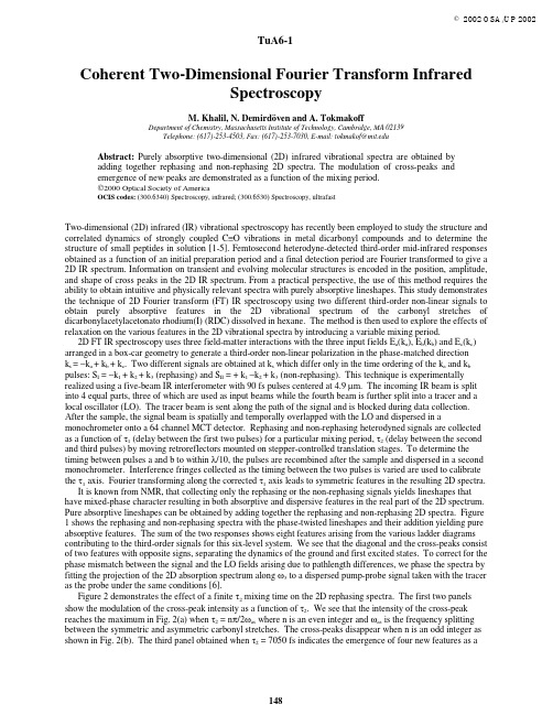
Coherent Two-Dimensional Fourier Transform InfraredSpectroscopyM.Khalil,N.Demirdöven and A.TokmakoffDepartment of Chemistry,Massachusetts Institute of Technology,Cambridge,MA02139Telephone:(617)-253-4503,Fax:(617)-253-7030,E-mail:tokmakof@Abstract:Purely absorptive two-dimensional(2D)infrared vibrational spectra are obtained byadding together rephasing and non-rephasing2D spectra.The modulation of cross-peaks andemergence of new peaks are demonstrated as a function of the mixing period.2000Optical Society of AmericaOCIS codes:(300.6340)Spectroscopy,infrared;(300.6530)Spectroscopy,ultrafastTwo-dimensional(2D)infrared(IR)vibrational spectroscopy has recently been employed to study the structure and correlated dynamics of strongly coupled C≡O vibrations in metal dicarbonyl compounds and to determine the structure of small peptides in solution[1-5].Femtosecond heterodyne-detected third-order mid-infrared responses obtained as a function of an initial preparation period and a final detection period are Fourier transformed to give a 2D IR rmation on transient and evolving molecular structures is encoded in the position,amplitude, and shape of cross peaks in the2D IR spectrum.From a practical perspective,the use of this method requires the ability to obtain intuitive and physically relevant spectra with purely absorptive lineshapes.This study demonstrates the technique of2D Fourier transform(FT)IR spectroscopy using two different third-order non-linear signals to obtain purely absorptive features in the2D vibrational spectrum of the carbonyl stretches of dicarbonylacetylacetonato rhodium(I)(RDC)dissolved in hexane.The method is then used to explore the effects of relaxation on the various features in the2D vibrational spectra by introducing a variable mixing period.2D FT IR spectroscopy uses three field-matter interactions with the three input fields E a(k a),E b(k b)and E c(k c) arranged in a box-car geometry to generate a third-order non-linear polarization in the phase-matched directionk s=−k a+k b+k c.Two different signals are obtained at k s which differ only in the time ordering of the k a and k b pulses:S I=−k1+k2+k3(rephasing)and S II=+k1−k2+k3(non-rephasing).This technique is experimentally realized using a five-beam IR interferometer with90fs pulses centered at4.9µm.The incoming IR beam is split into4equal parts,three of which are used as input beams while the fourth beam is further split into a tracer and a local oscillator(LO).The tracer beam is sent along the path of the signal and is blocked during data collection. After the sample,the signal beam is spatially and temporally overlapped with the LO and dispersed in a monochrometer onto a64channel MCT detector.Rephasing and non-rephasing heterodyned signals are collected as a function ofτ1(delay between the first two pulses)for a particular mixing period,τ2(delay between the second and third pulses)by moving retroreflectors mounted on stepper-controlled translation stages.To determine the timing between pulses a and b to withinλ/10,the pulses are recombined after the sample and dispersed in a second monochrometer.Interference fringes collected as the timing between the two pulses is varied are used to calibrate theτ1axis.Fourier transforming along the correctedτ1axis leads to symmetric features in the resulting2D spectra.It is known from NMR,that collecting only the rephasing or the non-rephasing signals yields lineshapes that have mixed-phase character resulting in both absorptive and dispersive features in the real part of the2D spectrum. Pure absorptive lineshapes can be obtained by adding together the rephasing and non-rephasing2D spectra.Figure 1shows the rephasing and non-rephasing spectra with the phase-twisted lineshapes and their addition yielding pure absorptive features.The sum of the two responses shows eight features arising from the various ladder diagrams contributing to the third-order signals for this six-level system.We see that the diagonal and the cross-peaks consist of two features with opposite signs,separating the dynamics of the ground and first excited states.To correct for the phase mismatch between the signal and the LO fields arising due to pathlength differences,we phase the spectra by fitting the projection of the2D absorption spectrum alongω3to a dispersed pump-probe signal taken with the tracer as the probe under the same conditions[6].Figure2demonstrates the effect of a finiteτ2mixing time on the2D rephasing spectra.The first two panels show the modulation of the cross-peak intensity as a function ofτ2.We see that the intensity of the cross-peak reaches the maximum in Fig.2(a)whenτ2=nπ/2ωas where n is an even integer andωas is the frequency splitting between the symmetric and asymmetric carbonyl stretches.The cross-peaks disappear when n is an odd integer as shown in Fig.2(b).The third panel obtained whenτ2=7050fs indicates the emergence of four new features as a200020502100-ω1/2πc (cm -1)200020502100200020502100(c)(b)(a)-ω1/2πc (cm -1)ωsωaωa ωs ωsωa ωa ωsω3/2πc (c m -1)200020502100ω1/2πc (cm -1)Fig.1.Real part of 2D IR vibrational spectra at τ2=0(a)S I (b)S II and (c)S I +S II .result of various coherent and incoherent population relaxation processes occurring during the mixing time.This results in the diagonal and cross-peaks splitting into three features instead of the usual two features obtained at smaller values of τ2.A systematic study of the 2D rephasing and non-rephasing spectra as a function of τ2allows us to map out the complete dynamics of this multi-level system including the effects of solvent-induced relaxation and populationrelaxation.ωs ωaω3/2πc (c m -1)-ω1/2πc (cm -1)Fig.2.Absolute value 2D IR rephasing spectra as a function of a variable mixing time.(a)τ2=470fs (b)τ2=705fs(c)τ2=7050fs.1.O.Golonzka,M.Khalil,N.Demirdöven,and A.Tokmakoff,“Coupling and orientation between anharmonic vibrations characterized by two-dimensional infrared vibrational spectroscopy,”J.Chem.Phys.,115,10814-10828(2001).2.N.Demirdöven,M.Khalil,O.Golonzka,and A.Tokmakoff,“Correlation effects in two-dimensional vibrational spectroscopy of coupled vibrations,”J.Phys.Chem.A,105,8025-8030(2001).3.D.E.Thompson,K.A.Merchant and M.D.Fayer,“Two-dimensional ultrafast infrared vibrational echo studies of solute-solvent interactionsand dynamics,”J.Chem.Phys.,115,317-330(2001).4.M.T.Zanni,S.Gnanakaran,J.Stenger,and R.M.Hochstrasser,“Heterodyned two-dimensional infrared spectroscopy of solvent-dependent conformations of acetylproline-NH2,”J.Phys.Chem.B,105,6520-6535(2001).5.S.Woutersen,and P.Hamm,“Structure determination of trialanine in water using polarization sensitive two-dimensional vibrational spectroscopy,”J.Phys.Chem.B,104,11316-11320(2000).6.J.D.Hybl,A.Albrecht Ferro and D.M.Jonas,“Two-dimensional Fourier transform electronic spectroscopy,”J.Chem.Phys.,115,6606-6622(2001).。

菲涅耳非相干关联全息图(综述)

Fresnel incoherent correlation hologram-a reviewInvited PaperJoseph Rosen,Barak Katz1,and Gary Brooker2∗∗1Department of Electrical and Computer Engineering,Ben-Gurion University of the Negev,P.O.Box653,Beer-Sheva84105,Israel2Johns Hopkins University Microscopy Center,Montgomery County Campus,Advanced Technology Laboratory, Whiting School of Engineering,9605Medical Center Drive Suite240,Rockville,MD20850,USA∗E-mail:rosen@ee.bgu.ac.il;∗∗e-mail:gbrooker@Received July17,2009Holographic imaging oﬀers a reliable and fast method to capture the complete three-dimensional(3D) information of the scene from a single perspective.We review our recently proposed single-channel optical system for generating digital Fresnel holograms of3D real-existing objects illuminated by incoherent light.In this motionless holographic technique,light is reﬂected,or emitted from a3D object,propagates througha spatial light modulator(SLM),and is recorded by a digital camera.The SLM is used as a beam-splitter of the single-channel incoherent interferometer,such that each spherical beam originated from each object point is split into two spherical beams with two diﬀerent curve radii.Incoherent sum of the entire interferences between all the couples of spherical beams creates the Fresnel hologram of the observed3D object.When this hologram is reconstructed in the computer,the3D properties of the object are revealed.OCIS codes:100.6640,210.4770,180.1790.doi:10.3788/COL20090712.0000.1.IntroductionHolography is an attractive imaging technique as it oﬀers the ability to view a complete three-dimensional (3D)volume from one image.However,holography is not widely applied to the regime of white-light imaging, because white-light is incoherent and creating holograms requires a coherent interferometer system.In this review, we describe our recently invented method of acquiring incoherent digital holograms.The term incoherent digi-tal hologram means that incoherent light beams reﬂected or emitted from real-existing objects interfere with each other.The resulting interferogram is recorded by a dig-ital camera and digitally processed to yield a hologram. This hologram is reconstructed in the computer so that 3D images appear on the computer screen.The oldest methods of recording incoherent holograms have made use of the property that every incoherent ob-ject is composed of many source points,each of which is self-spatial coherent and can create an interference pattern with light coming from the point’s mirrored image.Under this general principle,there are vari-ous types of holograms[1−8],including Fourier[2,6]and Fresnel holograms[3,4,8].The process of beam interfering demands high levels of light intensity,extreme stability of the optical setup,and a relatively narrow bandwidth light source.More recently,three groups of researchers have proposed computing holograms of3D incoherently illuminated objects from a set of images taken from diﬀer-ent points of view[9−12].This method,although it shows promising prospects,is relatively slow since it is based on capturing tens of scene images from diﬀerent view angles. Another method is called scanning holography[13−15],in which a pattern of Fresnel zone plates(FZPs)scans the object such that at each and every scanning position, the light intensity is integrated by a point detector.The overall process yields a Fresnel hologram obtained as a correlation between the object and FZP patterns.How-ever,the scanning process is relatively slow and is done by mechanical movements.A similar correlation is ac-tually also discussed in this review,however,unlike the case of scanning holography,our proposed system carries out a correlation without movement.2.General properties of Fresnel hologramsThis review concentrates on the technique of incoher-ent digital holography based on single-channel incoher-ent interferometers,which we have been involved in their development recently[16−19].The type of hologram dis-cussed here is the digital Fresnel hologram,which means that a hologram of a single point has the form of the well-known FZP.The axial location of the object point is encoded by the Fresnel number of the FZP,which is the technical term for the number of the FZP rings along the given radius.To understand the operation principle of any general Fresnel hologram,let us look on the diﬀerence between regular imaging and holographic systems.In classical imaging,image formation of objects at diﬀerent distances from the lens results in a sharp image at the image plane for objects at only one position from the lens,as shown in Fig.1(a).The other objects at diﬀerent distances from the lens are out of focus.A Fresnel holographic system,on the other hand,as depicted in Fig.1(b),1671-7694/2009/120xxx-08c 2009Chinese Optics Lettersprojects a set of rings known as the FZP onto the plane of the image for each and every point at every plane of the object being viewed.The depth of the points is en-coded by the density of the rings such that points which are closer to the system project less dense rings than distant points.Because of this encoding method,the 3D information in the volume being imaged is recorded into the recording medium.Thus once the patterns are decoded,each plane in the image space reconstructed from a Fresnel hologram is in focus at a diﬀerent axial distance.The encoding is accomplished by the presence of a holographic system in the image path.At this point it should be noted that this graphical description of pro-jecting FZPs by every object point actually expresses the mathematical two-dimensional (2D)correlation (or convolution)between the object function and the FZP.In other words,the methods of creating Fresnel holo-grams are diﬀerent from each other by the way they spatially correlate the FZP with the scene.Another is-sue to note is that the correlation should be done with a FZP that is somehow “sensitive”to the axial locations of the object points.Otherwise,these locations are not encoded into the hologram.The system described in this review satisﬁes the condition that the FZP is depen-dent on the axial distance of each and every objectpoint.parison between the Fresnel holography principle and conventional imaging.(a)Conventional imaging system;(b)fresnel holographysystem.Fig.2.Schematic of FINCH recorder [16].BS:beam splitter;L is a spherical lens with focal length f =25cm;∆λindicates a chromatic ﬁlter with a bandwidth of ∆λ=60nm.This means that indeed points,which are closer to the system,project FZP with less cycles per radial length than distant points,and by this condition the holograms can actually image the 3D scene properly.The FZP is a sum of at least three main functions,i.e.,a constant bias,a quadratic phase function and its complex conjugate.The object function is actually corre-lated with all these three functions.However,the useful information,with which the holographic imaging is real-ized,is the correlation with just one of the two quadratic phase functions.The correlation with the other quadratic phase function induces the well-known twin image.This means that the detected signal in the holographic system contains three superposed correlation functions,whereas only one of them is the required correlation between the object and the quadratic phase function.Therefore,the digital processing of the detected image should contain the ability to eliminate the two unnecessary terms.To summarize,the deﬁnition of Fresnel hologram is any hologram that contains at least a correlation (or convolu-tion)between an object function and a quadratic phase function.Moreover,the quadratic phase function must be parameterized according to the axial distance of the object points from the detection plane.In other words,the number of cycles per radial distance of each quadratic phase function in the correlation is dependent on the z distance of each object point.In the case that the object is illuminated by a coherent wave,this correlation is the complex amplitude of the electromagnetic ﬁeld directly obtained,under the paraxial approximation [20],by a free propagation from the object to the detection plane.How-ever,we deal here with incoherent illumination,for which an alternative method to the free propagation should be applied.In fact,in this review we describe such method to get the desired correlation with the quadratic phase function,and this method indeed operates under inco-herent illumination.The discussed incoherent digital hologram is dubbed Fresnel incoherent correlation hologram (FINCH)[16−18].The FINCH is actually based on a single-channel on-axis incoherent interferometer.Like any Fresnel holography,in the FINCH the object is correlated with a FZP,but the correlation is carried out without any movement and without multiplexing the image of the scene.Section 3reviews the latest developments of the FINCH in the ﬁeld of color holography,microscopy,and imaging with a synthetic aperture.3.Fresnel incoherent correlation holographyIn this section we describe the FINCH –a method of recording digital Fresnel holograms under incoher-ent illumination.Various aspects of the FINCH have been described in Refs.[16-19],including FINCH of re-ﬂected white light [16],FINCH of ﬂuorescence objects [17],a FINCH-based holographic ﬂuorescence microscope [18],and a hologram recorder in a mode of a synthetic aperture [19].We brieﬂy review these works in the current section.Generally,in the FINCH system the reﬂected incoher-ent light from a 3D object propagates through a spatial light modulator (SLM)and is recorded by a digital cam-era.One of the FINCH systems [16]is shown in Fig.2.White-light source illuminates a 3D scene,and the reﬂected light from the objects is captured by a charge-coupled device (CCD)camera after passing through a lens L and the SLM.In general,we regard the system as an incoherent interferometer,where the grating displayed on the SLM is considered as a beam splitter.As is com-mon in such cases,we analyze the system by following its response to an input object of a single inﬁnitesimal point.Knowing the system’s point spread function (PSF)en-ables one to realize the system operation for any general object.Analysis of a beam originated from a narrow-band inﬁnitesimal point source is done by using Fresnel diﬀraction theory [20],since such a source is coherent by deﬁnition.A Fresnel hologram of a point object is obtained when the two interfering beams are two spherical beams with diﬀerent curvatures.Such a goal is achieved if the SLM’s reﬂection function is a sum of,for instance,constant and quadratic phase functions.When a plane wave hits the SLM,the constant term represents the reﬂected plane wave,and the quadratic phase term is responsible for the reﬂected spherical wave.A point source located at some distance from a spher-ical positive lens induces on the lens plane a diverging spherical wave.This wave is split by the SLM into two diﬀerent spherical waves which propagate toward the CCD at some distance from the SLM.Consequently,in the CCD plane,the intensity of the recorded hologram is a sum of three terms:two complex-conjugated quadratic phase functions and a constant term.This result is the PSF of the holographic recording system.For a general 3D object illuminated by a narrowband incoherent illumination,the intensity of the recorded hologram is an integral of the entire PSFs,over all object intensity points.Besides a constant term,thehologramFig.3.(a)Phase distribution of the reﬂection masks dis-played on the SLM,with θ=0◦,(b)θ=120◦,(c)θ=240◦.(d)Enlarged portion of (a)indicating that half (randomly chosen)of the SLM’s pixels modulate light with a constant phase.(e)Magnitude and (f)phase of the ﬁnal on-axis digi-tal hologram.(g)Reconstruction of the hologram of the three characters at the best focus distance of ‘O’.(h)Same recon-struction at the best focus distance of ‘S’,and (i)of ‘A’[16].expression contains two terms of correlation between an object and a quadratic phase,z -dependent,function.In order to remain with a single correlation term out of the three terms,we follow the usual procedure of on-axis digital holography [14,16−19].Three holograms of the same object are recorded with diﬀerent phase con-stants.The ﬁnal hologram is a superposition of the three holograms containing only the desired correlation between the object function and a single z -dependent quadratic phase.A 3D image of the object can be re-constructed from the hologram by calculating theFresnelFig.4.Schematics of the FINCH color recorder [17].L 1,L 2,L 3are spherical lenses and F 1,F 2are chromaticﬁlters.Fig.5.(a)Magnitude and (b)phase of the complex Fres-nel hologram of the dice.Digital reconstruction of the non-ﬂuorescence hologram:(c)at the face of the red dots on the die,and (d)at the face of the green dots on the die.(e)Magnitude and (f)phase of the complex Fresnel hologram of the red dots.Digital reconstruction of the red ﬂuorescence hologram:(g)at the face of the red dots on the die,and (h)at the face of the green dots on the die.(i)Magnitude and (j)phase of the complex Fresnel hologram of the green dots.Digital reconstruction of the green ﬂuorescence hologram:(k)at the face of the red dots on the die,and (l)at the face of the green dots on the position of (c),(g),(k)and that of (d),(h),(l)are depicted in (m)and (n),respectively [17].Fig.6.FINCHSCOPE schematic in uprightﬂuorescence microscope[18].propagation formula.The system shown in Fig.2has been used to record the three holograms[16].The SLM has been phase-only, and as so,the desired sum of two phase functions(which is no longer a pure phase)cannot be directly displayed on this SLM.To overcome this obstacle,the quadratic phase function has been displayed randomly on only half of the SLM pixels,and the constant phase has been displayed on the other half.The randomness in distributing the two phase functions has been required because organized non-random structure produces unnecessary diﬀraction orders,therefore,results in lower interference eﬃciency. The pixels are divided equally,half to each diﬀractive element,to create two wavefronts with equal energy.By this method,the SLM function becomes a good approx-imation to the sum of two phase functions.The phase distributions of the three reﬂection masks displayed on the SLM,with phase constants of0◦,120◦and240◦,are shown in Figs.3(a),(b)and(c),respectively.Three white-on-black characters i th the same size of 2×2(mm)were located at the vicinity of rear focal point of the lens.‘O’was at z=–24mm,‘S’was at z=–48 mm,and‘A’was at z=–72mm.These characters were illuminated by a mercury arc lamp.The three holo-grams,each for a diﬀerent phase constant of the SLM, were recorded by a CCD camera and processed by a computer.Theﬁnal hologram was calculated accord-ing to the superposition formula[14]and its magnitude and phase distributions are depicted in Figs.3(e)and (f),respectively.The hologram was reconstructed in the computer by calculating the Fresnel propagation toward various z propagation distances.Three diﬀerent recon-struction planes are shown in Figs.3(g),(h),and(i).In each plane,a diﬀerent character is in focus as is indeed expected from a holographic reconstruction of an object with a volume.In Ref.[17],the FINCH has been capable to record multicolor digital holograms from objects emittingﬂuo-rescent light.Theﬂuorescent light,speciﬁc to the emis-sion wavelength of variousﬂuorescent dyes after excita-tion of3D objects,was recorded on a digital monochrome camera after reﬂection from the SLM.For each wave-length ofﬂuorescent emission,the camera sequentially records three holograms reﬂected from the SLM,each with a diﬀerent phase factor of the SLM’s function.The three holograms are again superposed in the computer to create a complex-valued Fresnel hologram of eachﬂu-orescent emission without the twin image problem.The holograms for eachﬂuorescent color are further combined in a computer to produce a multicoloredﬂuorescence hologram and3D color image.An experiment showing the recording of a colorﬂuo-rescence hologram was carried out[17]on the system in Fig. 4.The phase constants of0◦,120◦,and240◦were introduced into the three quadratic phase functions.The magnitude and phase of theﬁnal complex hologram,su-perposed from theﬁrst three holograms,are shown in Figs.5(a)and(b),respectively.The reconstruction from theﬁnal hologram was calculated by using the Fresnel propagation formula[20].The results are shown at the plane of the front face of the front die(Fig.5(c))and the plane of the front face of the rear die(Fig.5(d)).Note that in each plane a diﬀerent die face is in focus as is indeed expected from a holographic reconstruction of an object with a volume.The second three holograms were recorded via a redﬁlter in the emissionﬁlter slider F2 which passed614–640nmﬂuorescent light wavelengths with a peak wavelength of626nm and a full-width at half-maximum,of11nm(FWHM).The magnitude and phase of theﬁnal complex hologram,superposed from the‘red’set,are shown in Figs.5(e)and(f),respectively. The reconstruction results from thisﬁnal hologram are shown in Figs.5(g)and(h)at the same planes as those in Figs.5(c)and(d),respectively.Finally,an additional set of three holograms was recorded with a greenﬁlter in emissionﬁlter slider F2,which passed500–532nmﬂuo-rescent light wavelengths with a peak wavelength of516 nm and a FWHM of16nm.The magnitude and phase of theﬁnal complex hologram,superposed from the‘green’set,are shown in Figs.5(i)and(j),respectively.The reconstruction results from thisﬁnal hologram are shown in Figs.5(k)and(l)at the same planes as those in Fig. 5(c)and(d),positions of Figs.5(c), (g),and(k)and Figs.5(d),(h),and(l)are depicted in Figs.5(m)and(n),respectively.Note that all the colors in Fig.5(colorful online)are pseudo-colors.These last results yield a complete color3D holographic image of the object including the red and greenﬂuorescence. While the optical arrangement in this demonstration has not been optimized for maximum resolution,it is im-portant to recognize that even with this simple optical arrangement,the resolution is good enough to image the ﬂuorescent emissions with goodﬁdelity and to obtain good reﬂected light images of the dice.Furthermore, in the reﬂected light images in Figs.5(c)and(m),the system has been able to detect a specular reﬂection of the illumination from the edge of the front dice. Another system to be reviewed here is theﬁrst demon-stration of a motionless microscopy system(FINCH-SCOPE)based upon the FINCH and its use in record-ing high-resolution3Dﬂuorescent images of biological specimens[18].By using high numerical aperture(NA) lenses,a SLM,a CCD camera,and some simpleﬁlters, FINCHSCOPE enables the acquisition of3D microscopic images without the need for scanning.A schematic diagram of the FINCHSCOPE for an upright microscope equipped with an arc lamp sourceFig.7.FINCHSCOPE holography of polychromatic beads.(a)Magnitude of the complex hologram 6-µm beads.Images reconstructed from the hologram at z distances of (b)34µm,(c)36µm,and (d)84µm.Line intensity proﬁles between the beads are shown at the bottom of panels (b)–(d).(e)Line intensity proﬁles along the z axis for the lower bead from reconstructed sections of a single hologram (line 1)and from a wideﬁeld stack of the same bead (28sections,line 2).Beads (6µm)excited at 640,555,and 488nm with holograms reconstructed (f)–(h)at plane (b)and (j)–(l)at plane (d).(i)and (m)are the combined RGB images for planes (b)and (d),respectively.(n)–(r)Beads (0.5µm)imaged with a 1.4-NA oil immersion objective:(n)holographic camera image;(o)magnitude of the complex hologram;(p)–(r)reconstructed image at planes 6,15,and 20µm.Scale bars indicate image size [18].Fig.8.FINCHSCOPE ﬂuorescence sections of pollen grains and Convallaria rhizom .The arrows point to the structures in the images that are in focus at various image planes.(b)–(e)Sections reconstructed from a hologram of mixed pollen grains.(g)–(j)Sections reconstructed from a hologram of Convallaria rhizom .(a),(f)Magnitudes of the complex holograms from which the respective image planes are reconstructed.Scale bars indicate image size [18].is shown in Fig. 6.The beam of light that emerges from an inﬁnity-corrected microscope objective trans-forms each point of the object being viewed into a plane wave,thus satisfying the ﬁrst requirement of FINCH [16].A SLM and a digital camera replace the tube lens,reﬂec-tive mirror,and other transfer optics normally present in microscopes.Because no tube lens is required,inﬁnity-corrected objectives from any manufacturer can be used.A ﬁlter wheel was used to select excitation wavelengths from a mercury arc lamp,and the dichroic mirror holder and the emission ﬁlter in the microscope were used to direct light to and from the specimen through an inﬁnity-corrected objective.The ability of the FINCHSCOPE to resolve multicolor ﬂuorescent samples was evaluated by ﬁrst imaging poly-chromatic ﬂuorescent beads.A ﬂuorescence bead slidewith the beads separated on two separate planes was con-structed.FocalCheck polychromatic beads(6µm)were used to coat one side of a glass microscope slide and a glass coverslip.These two surfaces were juxtaposed and held together at a distance from one another of∼50µm with optical cement.The beads were sequentially excited at488-,555-,and640-nm center wavelengths(10–30nm bandwidths)with emissions recorded at515–535,585–615,and660–720nm,respectively.Figures7(a)–(d) show reconstructed image planes from6µm beads ex-cited at640nm and imaged on the FINCHSCOPE with a Zeiss PlanApo20×,0.75NA objective.Figure7(a) shows the magnitude of the complex hologram,which contains all the information about the location and in-tensity of each bead at every plane in theﬁeld.The Fresnel reconstruction from this hologram was selected to yield49planes of the image,2-µm apart.Two beads are shown in Fig.7(b)with only the lower bead exactly in focus.Figure7(c)is2µm into theﬁeld in the z-direction,and the upper bead is now in focus,with the lower bead slightly out of focus.The focal diﬀerence is conﬁrmed by the line proﬁle drawn between the beads, showing an inversion of intensity for these two beads be-tween the planes.There is another bead between these two beads,but it does not appear in Figs.7(b)or(c) (or in the intensity proﬁle),because it is48µm from the upper bead;it instead appears in Fig.7(d)(and in the line proﬁle),which is24sections away from the section in Fig.7(c).Notice that the beads in Figs.7(b)and(c)are no longer visible in Fig.7(d).In the complex hologram in Fig.7(a),the small circles encode the close beads and the larger circles encode the distant central bead. Figure7(e)shows that the z-resolution of the lower bead in Fig.7(b),reconstructed from sections created from a single hologram(curve1),is at least comparable to data from a wideﬁeld stack of28sections(obtained by moving the microscope objective in the z-direction)of the same ﬁeld(curve2).The co-localization of theﬂuorescence emission was conﬁrmed at all excitation wavelengths and at extreme z limits,as shown in Figs.7(f)–(m)for the 6-µm beads at the planes shown in Figs.7(b)((f)–(i)) and(d)((j)–(m)).In Figs.7(n)–(r),0.5-µm beads imaged with a Zeiss PlanApo×631.4NA oil-immersion objective are shown.Figure7(n)presents one of the holo-grams captured by the camera and Fig.7(o)shows the magnitude of the complex hologram.Figures7(p)–(r) show diﬀerent planes(6,15,and20µm,respectively)in the bead specimen after reconstruction from the complex hologram of image slices in0.5-µm steps.Arrows show the diﬀerent beads visualized in diﬀerent z image planes. The computer reconstruction along the z-axis of a group ofﬂuorescently labeled pollen grains is shown in Figs. 8(b)–(e).As is expected from a holographic reconstruc-tion of a3D object with volume,any number of planes can be reconstructed.In this example,a diﬀerent pollen grain was in focus in each transverse plane reconstructed from the complex hologram whose magnitude is shown in Fig.8(a).In Figs.8(b)–(e),the values of z are8,13, 20,and24µm,respectively.A similar experiment was performed with the autoﬂuorescent Convallaria rhizom and the results are shown in Figs.8(g)–(j)at planes6, 8,11,and12µm.The most recent development in FINCH is a new lens-less incoherent holographic system operating in a syn-thetic aperture mode[19].Synthetic aperture is a well-known super-resolution technique which extends the res-olution capabilities of an imaging system beyond thetheoretical Rayleigh limit dictated by the system’s ac-tual ing this technique,several patternsacquired by an aperture-limited system,from variouslocations,are tiled together to one large pattern whichcould be captured only by a virtual system equippedwith a much wider synthetic aperture.The use of optical holography for synthetic apertureis usually restricted to coherent imaging[21−23].There-fore,the use of this technique is limited only to thoseapplications in which the observed targets can be illu-minated by a laser.Synthetic aperture carried out by acombination of several oﬀ-axis incoherent holograms inscanning holographic microscopy has been demonstratedby Indebetouw et al[24].However,this method is limitedto microscopy only,and although it is a technique ofrecording incoherent holograms,a specimen should alsobe illuminated by an interference pattern between twolaser beams.Our new scheme of holographic imaging of incoher-ently illuminated objects is dubbing a synthetic aperturewith Fresnel elements(SAFE).This holographic lens-less system contains only a SLM and a digital camera.SAFE has an extended synthetic aperture in order toimprove the transverse and axial resolutions beyond theclassic limitations.The term synthetic aperture,in thepresent context,means time(or space)multiplexing ofseveral Fresnel holographic elements captured from vari-ous viewpoints by a system with a limited real aperture.The synthetic aperture is implemented by shifting theSLM-camera set,located across theﬁeld of view,be-tween several viewpoints.At each viewpoint,a diﬀerentmask is displayed on the SLM,and a single element ofthe Fresnel hologram is recorded(Fig.9).The variouselements,each of which is recorded by the real aperturesystem during the capturing time,are tiled together sothat theﬁnal mosaic hologram is eﬀectively consideredas being captured from a single synthetic aperture,whichis much wider than the actual aperture.An example of such a system with the synthetic aper-ture three times wider than the actual aperture can beseen in Fig.9.For simplicity of the demonstration,the synthetic aperture was implemented only along thehorizontal axis.In principle,this concept can be gen-eralized for both axes and for any ratio of synthetic toactual apertures.Imaging with the synthetic apertureis necessary for the cases where the angular spectrumof the light emitted from the observed object is widerthan the NA of a given imaging system.In the SAFEshown in Fig.9,the SLM and the digital camera movein front of the object.The complete Fresnel hologramof the object,located at some distance from the SLM,isa mosaic of three holographic elements,each of which isrecorded from a diﬀerent position by the system with thereal aperture of the size A x×A y.The complete hologram tiled from the three holographic Fresnel elements has thesynthetic aperture of the size3(·A x×A y)which is three times larger than the real aperture at the horizontal axis.The method to eliminate the twin image and the biasterm is the same as that has been used before[14,16−18];。

美国电气设备 ProLine UL 67 面板板和断言器说明书

—US C ATALOGProLineUL 67 Panelboards and breakers—Table of contents04D escription and features 07C atalog number guide andpanelboard configurator 08Order codes09Breakers14Accessories15A pproximate dimensions 18T echnical specifications 19S eries UL ratings21 B reaker placement guide4PROLINE PANELBOARD AND BREAKERS—ProLine panelboard and breakers descriptionElectrical• UL File #E499134• UL 67• 225 A and 400 A• 42 and 84 circuits (12- and 24-circuit types upon request)• Panelboard rating 480Y/277 V AC, branch breaker rating480Y/277 V AC up to 35 A and 240 V AC up to 100 A• Up to 35 kAIC series rating @240 V AC• Up to 30 kAIC series rating @480Y/277 V AC• Single- or double-ended (feed-through)• 1 A to 100 A branch breakers• Fully rated sub-fed lugs or breaker• NEMA 1 enclosure optionalFeatures• Breakers UL current-limiting• Fully coordinated• IP20 touch-safe• Pluggable breaker with non-energized bolt-on screwElectrical• Current-limiting according to UL 489• Up to 240 V and 480Y/277 V AC• Stand-alone rating up to 50 kA (depending on breaker type)• K trip curve• 1 A to 100 AFeatures• Contact position window• Independent thermal and magnetic trip units• Branch breakers with separated electrical (plug-in)and mechanical (bolt-on) connectionThe ProLine branch circuit breakers are the industry’s first UL listedcurrent-limiting breakers to be used in a panelboard application.The ProLine panelboard is the electrical industry’s first current-limiting, touch-safe and fully coordinated UL 67 panelboard.5DESCRIPTION AND FEATURES —Panelboard featuresMain breakerMain incoming connections• Lugs• Breaker• Studs Touch-safe main cover• Removable maincover with integratedneutral terminals• Access to neutralconnections withoutremoving coverNeutral bar assembly (with touch-safe cover)Branch breakers• 1 A to 100 A @ 240 V AC•1 A to 35 A @ 480Y/277 V AC6PROLINE PANELBOARD AND BREAKERS—Breaker featuresStable busbar design for high withstand ratings• Busbar designed with more surface area than typical panelboard busbar• Busbar encased in resin to aid stabilization in case of a faultNon-energizedmechanicalbolt-onconnection Electrical plug-in connectionPluggable with non-energized bolt-on connectionBreaker bus connection pointNon-energizedbolt-on pointEncased busbarsRecessedtouch-safebreakerconnectionInsulatingresin71 12-circuit version not available with double incoming.C ATA LO G N U M B ER G U IDE A N D PA N EL B OA R D CO N FI G U R ATO R —Catalog number guide and panelboard configurator1–2 – Product prefix Proline order code explanationA complete Proline part number consists of 14 characters.All characters shown are mandatory.4-5– Circuits 11 – Type13-14 – Enclosure—1–2 – Product prefix —3 – Phases —4-5 – Circuits —8-10 – AmpacityCode —Mandatory characters—6 – Incoming —13-14 – Enclosure —7 – Main —11 – Type—12 – Neutral7 – Main8PROLINE PANELBOARD AND BREAKERS—ProLine panelboard standard order codesCatalog number Description9BREAKERS —Branch breakersSUP200M seriesRated current I n Rated current I nSUP201MSUP202MSUP203MPROLINE PANELBOARD AND BREAKERSRated current I n Rated current I n Available with ring tongue terminals upon request.S801U S802U S803U11BREAKERS —Bus connectors for branch breakersCatalog number DescriptionPLBCS2PLBCS8L2R PLBCS8L1L PLBCS8L3RPLBCS8L2L PLBCS8DL1PLBCS8L3LPLBCS8DL2PLBCS8L1R PLBCS8DL312PROLINE PANELBOARD AND BREAKERS—ProLine breakers 120, 208, 240 V AC (factory-assembled with bus connector)PLU700M120/208/240 V ACK curve, 1-poleK curve, 2-poleK curve, 3-polePLU701MPLU702M-K60LPLU703M-K100RPLU703M13480Y/277 V ACK curve, 1-poleK curve, 2-pole K curve, 3-poleBREAKERS —ProLine breakers 480Y /277 V AC, UL 489PLU700M14PROLINE PANELBOARD AND BREAKERS—Accessories — panelboardPanelboard chassis hole bus coverDescriptionCatalog numberNeutral and ground bar assembliesDescriptionCatalog numberNeutral/ground lugsDescriptionCatalog numberPLBUSCVRMain and sub-feed lugsLugs for incoming and outgoing connectionsDescriptionCatalog numberPL350MECLUGMains cover (incomer and neutral lugs)Description Catalog numberPLMCVR15—Approximate dimensionsPanelboards single-ended and double-ended42-Circuit, single-endedDimensions in inches.84-Circuit, single-ended42-Circuit, double-endedACCE SSO R I E S , A PPR OX I M ATE D I M ENSI O NS16PROLINE PANELBOARD AND BREAKERS PLU700M1 A–50 A—Approximate dimensionsPL700 breakersDimensions in inches.1.057PLU700M25 A L/R - 70 A L/RPROLINE PANELBOARD AND BREAKERS 17A PPR OX I M ATE D I M ENSI ONS 0.199PLU700M 80 A - 100 A—Approximate dimensions PL700 breakersDimensions in inches.18PROLINE PANELBOARD AND BREAKERS—Technical specificationsSUP200M, PLU700M, S800U and PL700-K breakersItem SUP200M/PLU700M SUP200M/PLU700M S800U/PL700-K (L) S800U/PL700-K (R)UL ratings489489489 Number of poles1, 2, 31, 2, 31, 2, 3 Tripping characteristic K K K Rated currents 1 to 35 A40 A, 50 A25 A to 70 A1, 80 to 100 A2 Minimum operating voltage12 V12 V12 V UL rated voltage and interrupting capacityStand-alone short circuit current rating 14 kA 10 kA 30 kA: Single pole50 kA: Multi-poleFrequency50/60 Hz50/60 Hz50/60 Hz Rated voltage480Y/277 V AC240 V AC240 V AC Protection category IP 20IP 20 IP 20 Main terminalsWire size18–16 AWG/13.3 in-lbs.18–4 AWG/0.75–25 mm225–1 AWG14–10 AWG/17.7 in-lbs.8–4 AWG/39.8 in-lbs.Torque25 in-lbs/2.8 Nm25 in-lbs/2.8 Nm35 in-lbs./4 Nm Tool#2 Posidrive#2 Posidrive#2 Posidrive Service life at rated load6,000 operations6,000 operations6,000 operations20,000 operations (Mechanical endurance)20,000 operations(Mechanical endurance)—Ambient temperaturesMinimum-25 °C -13 °F-25 °C -13 °F-25 °C -13 °F Maximum+55 °C 131 °F+55 °C 131 °F60 °C 140 °F Storage temperaturesMinimum-40 °C -40 °F-40 °C -40 °F-40 °C -40 °F Maximum70 °C 158 °F70 °C 158 °F70 °C 158 °FShock resistance25 g minimum of 2 impacts,shock duration of 13 ms 25 g minimum of 2 impacts,shock duration of 13 ms—Vibration resistance 5 g, 20 cycles, 5 Hz,150 Hz at 0.8 ln 5 g, 20 cycles, 5 Hz,150 Hz at 0.8 ln—1 60 A/70 A have different dimensions.2 80 A/90 A/100 A available as “R” only and have double stab adapters.PROLINE PANELBOARD AND BREAKERS19TECH N I C A L SPECI FI C ATI O NS, SER I E S U L R ATI N G S—Series UL ratingsSUP200M MCBs with SACE® Tmax® XT MCCBsMain breaker Branch breaker Interrupting rating Type Amps Poles Type, trip curve Amps Poles Rms sym. A V AC Phase20PROLINE PANELBOARD AND BREAKERS—Breaker placement guide PLU701MPLU702M-K60L PLU703M-K100RPLU700M 1 A-50 A (1P/2P/3P)PLU700M"L" 25 A-70 A (1P/2P/3P)PLU700M 1 A-50 A (1P/2P/3P)PLU700M"L" 25 A-50 A (1P/2P/3P)PLU700M 1 A-50 A (1P/2P/3P)PLU700M"R" 25 A-70 A (1P/2P/3P)PLU700M"R" 80A/90A/100A (1P/2P/3P)PLU700M 1 A-50 A (1P/2P/3P)PLU700M"L" 25 A-70 A (1P/2P/3P)PLU700M 1 A-50 A (1P/2P/3P)PLU700M"R" 25 A-50 A (1P/2P/3P)PLU700M 1 A-50 A (1P/2P/3P)PLU700M"R" 25 A-70 A (1P/2P/3P)PLU700M"R" 80A/90A/100A (1P/2P/3P)PLU703MNotes:• PLU70XM-R and L have differentstab adapter position dimensions(see dimension drawings)• PLU70XM-R 80 A/90 A/100 A-Have double stab adapters-Are available as R onlySER I E S U L R ATI N G S, B R E A K ER PL ACEM ENT G U I D EPROLINE PANELBOARD AND BREAKERS21—Notes22PROLINE PANELBOARD AND BREAKERS —We reserve the right to make technical changes or modify the contents of this document without prior notice. With regard to purchase orders, the agreed particulars shall prevail. ABB Inc. does not acceptany r esponsibility whatsoever for potential errors or possible lack of information in this document.We reserve all rights in this document and in thesubject matter and illustrations contained therein.Any reproduction or utilization of its contents – inwhole or in parts – is forbidden without prior written consent of ABB Inc.Copyright© 2022 ABB Inc.All rights reserved1S X U 400139C 0201 R E V .D A U G U S T 2022—ABB Inc.Electrification860 Ridge Lake Blvd.Memphis, TN 38120/lowvoltageCustomer Service: 800-816-78097:00 a.m. - 5:30 p.m., CST, Monday-Friday ********************.comTechnical Support: 888-385-1221, Option 17:00 a.m. - 5:00 p.m., CST, Monday-Friday *******************.com。

Two_Dimensional_Phase_Unwrapping_Final

Two-Dimensional Phase Unwrapping ProblemBy Dr. Munther Gdeisat and Dr. Francis LilleyPre-requisite:In order to understand this tutorial it is necessary for you to have already studied and completed the “one-dimensional phase unwrapping problem” tutorial before reading this document. There are many applications that produce wrapped phase images. Examples of these are synthetic aperture radar (SAR), magnetic resonance imaging (MRI) and fringe pattern analysis. The wrapped phase images that are produced by these applications are not usable unless they are first unwrapped so as to form a continuous phase map. This means that the development of a robust phase unwrapping algorithm is an important topic for all these applications. In this article, we will not discuss phase unwrapping only in the specific context of these applications, but we will instead explain the concept of the 2D phase unwrapping problem in general terms.1.Introduction to 2D phase unwrappingWe shall explain the 2D phase unwrapping process as follows. Suppose that we have a computer-generated continuous phase image that does not contain any phase wraps (2π jumps). This image may be displayed as a visual intensity array, as shown in Figure 1(a). The same image may also be plotted as a 3D surface, as shown in Figure 1(b). The intensities from a single row of this image (row 410) are graphically plotted in Figure 1(c). The Matlab code that is used to generate this phase image is as follows. The peaks Matlab function is used to generate the continuous phase image. Please note that we are using the term “continuous” here to refer not to an analogue signal, but to a discrete 1D phase signal, or a discrete 2D phase image, that does not contain any phase wraps.%This program is to simulate a continuous phase distribution to act as a dataset %for use in the 2D phase unwrapping problemclc; close all; clearN = 512;[x,y]=meshgrid(1:N);image1 = 2*peaks(N) + 0.1*x + 0.01*y;figure, colormap(gray(256)), imagesc(image1)title('Continuous phase image displayed as a visual intensity array')xlabel('Pixels'), ylabel('Pixels')figuresurf(image1,'FaceColor','interp', 'EdgeColor','none', 'FaceLighting','phong')view(-30,30), camlight left, axis tighttitle(' Continuous phase map image displayed as a surface plot')xlabel('Pixels'), ylabel('Pixels'), zlabel('Phase in radians')figure, plot(image1(410,:))title('Row 410 of the continuous phase image')xlabel('Pixels'), ylabel('Phase in radians')(a) (b) (c)Figure 1: (a) A computer-generated continuous phase image displayed as a visual intensity array, (b) thesame image plotted as a surface, (c) intensities from row 410 of the phase image. Now let us wrap the computer-generated continuous phase image. The Matlab code to perform this task is as follows;%wrap the 2D imageimage1_wrapped = atan2(sin(image1), cos(image1)); figure, colormap(gray(256)), imagesc(image1_wrapped)title('Wrapped phase image displayed as a visual intensity array') xlabel('Pixels'), ylabel('Pixels')figuresurf(image1_wrapped,'FaceColor','interp', 'EdgeColor','none', 'FaceLighting','phong')view(-30,70), camlight left , axis tighttitle('Wrapped phase image plotted as a surface')xlabel('Pixels'), ylabel('Pixels'), zlabel('Phase in radians')figure, plot(image1_wrapped(410,:))title('Row 410 of the wrapped phase image') xlabel('Pixels'), ylabel('Phase in radians')The wrapped image is shown below.PixelsP i x e l s5010015020025030035040045050050100150200250300350400450500PixelsP h a s e i n r a d i a n s(a) (b) (c)Figure 2: (a) A wrapped phase image displayed as a visual intensity array, (b) the wrapped image plotted asa surface, (c) row 410 of the wrapped phase image. Recall from the 1D phase unwrapping tutorial, that when we were dealing with lines of phase values, the phase wraps appeared as multiple 2π jumps forming a saw-tooth waveform like that shown in Figure 2(c). Note that in the 2D case, where we now have phase images in the form of a 2D array, the phase wraps appear as contour curves, as shown in Figure 2(a), which we shall refer to as wrap curves. These curves will appear in the form of either closed, or open, curves and you can see both types of curve in Figure 2(a). Note that in the latter case, if an open curve enters a wrapped phase image, it must therefore also leave it. In order to unwrap the image we can use the Itoh 2D phase unwrapper. There are two main methods by which the Itoh 2D phase unwrapper may be implemented. The first method involves unwrapping the rows in the wrapped image sequentially (one at a time). This produces an intermediate image that is only partially phase unwrapped. Next we perform a similar process, but this time unwrap all the columns within the partially unwrapped image. The resultant unwrapped phase image, as produced by this first implementation of the Itoh unwrapper, is shown in Figures 3(a) & (b). The Matlab code to perform this task is as follows.%Unwrap the image using the Itoh algorithm: the first method is performed %by first sequentially unwrapping the all rows, one at a time. image1_unwrapped = image1_wrapped; for i=1:Nimage1_unwrapped(i,:) = unwrap(image1_unwrapped(i,:)); end%Then sequentially unwrap all the columns one at a time for i=1:Nimage1_unwrapped(:,i) = unwrap(image1_unwrapped(:,i)); endfigure, colormap(gray(256)), imagesc(image1_unwrapped)title('Unwrapped phase image using the Itoh algorithm: the first method') xlabel('Pixels'), ylabel('Pixels')figuresurf(image1_unwrapped,'FaceColor','interp', 'EdgeColor','none', 'FaceLighting','phong')view(-30,30), camlight left , axis tighttitle('Unwrapped phase image using the Itoh algorithm: the first method') xlabel('Pixels'), ylabel('Pixels'), zlabel('Phase in radians')PixelsP i x e l s5010015020025030035040045050050100150200250300350400450500PixelsP h a s e i n r a d i a n sThe second method of implementing the Itoh unwrapper simply works the other way around. In other words, it involves first unwrapping all the columns within the wrapped phase image, one at a time. And this again produces a partially phase unwrapped image. Then we sequentially unwrap all rows of the partially unwrapped image. The resultant unwrapped phase image, produced using this second implementation of the Itoh unwrapper, is shown in Figure 3(b). The Matlab code to perform this task is as follows.%Unwrap the image using the Itoh algorithm: the second method%performed by first sequentially unwrapping all the columns one at a time. image2_unwrapped = image1_wrapped; for i=1:Nimage2_unwrapped(:,i) = unwrap(image2_unwrapped(:,i)); end%Then sequentially unwrap all the a rows one at a time for i=1:Nimage2_unwrapped(i,:) = unwrap(image2_unwrapped(i,:)); endfigure, colormap(gray(256)), imagesc(image2_unwrapped)title('Unwrapped phase image using Itoh algorithm: the second method') xlabel('Pixels'), ylabel('Pixels')figuresurf(image2_unwrapped,'FaceColor','interp', 'EdgeColor','none', 'FaceLighting','phong')view(-30,30), camlight left , axis tighttitle('Unwrapped phase image using the Itoh algorithm: the second method') xlabel('Pixels'), ylabel('Pixels'), zlabel('Phase in radians')(a)(b)(c)(d)Figure 3: Unwrapped image using the 2D Itoh algorithm; implemented using the first method in (a) & (b),and implemented using the second method in (c) & (d).PixelsP i x e l s5010015020025030035040045050050100150200250300350400450500unwrapped imagePixelsP i x e l s5010015020025030035040045050050100150200250300350400450500It is obvious from the exercise that has been performed above that both of these implementations of the Itoh phase unwrapping algorithm actually produce the same output. This is because this wrapped phase image is not a real one, but is instead an artificial dataset that does not contain any errors.The wrapped phase image that is shown in Figure 2(a) is a good example of an ideal phase image that does not contain any sources of error. We can easily process this image using any 2D phase unwrapper. As has been explained above, in this case we have processed the image using the 2D Itoh algorithm. This is a very simple phase unwrapping algorithm, which only works in cases where the phase images are virtually error free. Most real-world applications produce wrapped phase images that do contain errors. In this case, we need to use more complex 2D phase unwrappers in order to deal with these images.In 2D phase unwrapping, there are four sources of errors that complicate the phase unwrapping process. These sources of errors are as follows.1.Noise2.Under sampling3.When the continuous phase image contains sudden, abrupt phase changes4.Errors produced by the phase extraction algorithm itselfIn this tutorial we will discuss only the first three sources of errors and their effects upon the 2D phase unwrapping process. We will also explain how to successfully unwrap images in these three different situations. The fourth source of error depends on the specific algorithm that is used to extract the wrapped phase. The reader should be aware of this as another potential source of error when performing phase unwrapping, however a detailed discussion of the effects of an algorithm itself on the extracted wrapped phase is out of the scope of this tutorial and will not be covered here.2.The effect of noise on two-dimensional phase unwrappingA phase unwrapper detects the existence of a phase wrap in an image by calculating the difference between two successive samples. If this difference is larger than +π, then the phase unwrapper considers there to be a wrap at this location. This could either be a genuine phase wrap, or it could actually be a fake wrap due to the presence of noise. To study the effect of noise on 2D phase unwrapping, let us add noise to the simulated continuous phase image that was shown previously in Figure 1(a). Then we shall wrap the noisy phase image. After that, we will attempt to phase unwrap the simulated object. This process is implemented in the Matlab program that is shown below. The noise variance is set here to a value of 0.4. As we can see from Figure 4, such a low level of added noise does not adversely affect the operation of the Itoh unwrapping algorithm.%This program shows the problems encountered when unwrapping a noisy 2D phase%image by using computer simulationclc; close all; clearN = 512;[x,y]=meshgrid(1:N);noise_variance = 0.4;image1 = 2*peaks(N) + 0.1*x + 0.01*y + noise_variance*randn(N,N);figure, colormap(gray(256)), imagesc(image1)title('Noisy continuous phase image displayed as visual intensity array')xlabel('Pixels'), ylabel('Pixels')figuresurf(image1,'FaceColor','interp', 'EdgeColor','none', 'FaceLighting','phong')view(-30,30), camlight left, axis tighttitle('Noisy continuous phase image displayed as a surface plot')xlabel('Pixels'), ylabel('Pixels'), zlabel('Phase in radians')figure, plot(image1(410,:))title('Row 410 of the original noisy continuous phase image')xlabel('Pixels'), ylabel('Phase in radians')%wrap the 2D imageimage1_wrapped = atan2(sin(image1), cos(image1));figure, colormap(gray(256)), imagesc(image1_wrapped)title('Noisy wrapped phase image displayed as visual intensity array')xlabel('Pixels'), ylabel('Pixels')figuresurf(image1_wrapped,'FaceColor','interp', 'EdgeColor','none','FaceLighting','phong')view(-30,70), camlight left, axis tighttitle('Noisy wrapped phase image plotted as a surface plot')xlabel('Pixels'), ylabel('Pixels'), zlabel('Phase in radians')figure, plot(image1_wrapped(410,:))title('Row 410 of the wrapped noisy image')xlabel('Pixels'), ylabel('Phase in radians')%Unwrap the image using the Itoh algorithm: the first method%Unwrap the image first by sequentially unwrapping the rows one at a time.image1_unwrapped = image1_wrapped;for i=1:Nimage1_unwrapped(i,:) = unwrap(image1_unwrapped(i,:));end%Then unwrap all the columns one-by-onefor i=1:Nimage1_unwrapped(:,i) = unwrap(image1_unwrapped(:,i));endfigure, colormap(gray(256)), imagesc(image1_unwrapped)title('Unwrapped noisy phase image using the Itoh algorithm: the first method') xlabel('Pixels'), ylabel('Pixels')figuresurf(image1_unwrapped,'FaceColor','interp', 'EdgeColor','none','FaceLighting','phong')view(-30,30), camlight left, axis tighttitle('Unwrapped noisy phase image using the Itoh unwrapper: the first method') xlabel('Pixels'), ylabel('Pixels'), zlabel('Phase in radians')%Unwrap the image using the Itoh algorithm: the second method%Unwrap the image by first sequentially unwrapping all the columns.image2_unwrapped = image1_wrapped;for i=1:Nimage2_unwrapped(:,i) = unwrap(image2_unwrapped(:,i));end%Then unwrap all the a rows one-by-onefor i=1:Nimage2_unwrapped(i,:) = unwrap(image2_unwrapped(i,:));endfigure, colormap(gray(256)), imagesc(image2_unwrapped)title('Unwrapped noisy image using the Itoh algorithm: the second method')xlabel('Pixels'), ylabel('Pixels')figuresurf(image2_unwrapped,'FaceColor','interp', 'EdgeColor','none','FaceLighting','phong')view(-30,30), camlight left, axis tighttitle('Unwrapped noisy phase image using the Itoh algorithm: the second method') xlabel('Pixels'), ylabel('Pixels'), zlabel('Phase in radians')Figure 4: (a) & (b) A noisy computer-generated continuous phase image. (c) & (d) The noisy phase image is wrapped. (e) & (f) Phase unwrapping using the Itoh algorithm: first method. (g) & (h) Phase unwrapping using the Itoh algorithm: second method. The noise variance is set here to a value of 0.4.PixelsP i x e l s5010015020025030035040045050050100150200250300350400450500Wrapped image displayed as visual intensity arrayPixelsP i x e l s5010015020025030035040045050050100150200250300350400450500unwrapped image using the first methodPixelsP i x e l s5010015020025030035040045050050100150200250300350400450500unwrapped image using the second methodPixelsP i x e l s5010015020025030035040045050050100150200250300350400450500Figure 5: (a) & (b) A noisy computer-generated continuous phase image. (c) & (d) The noisy phase image is wrapped. (e) & (f) Phase unwrapping using the Itoh algorithm: first method. (g) & (h) Phase unwrapping using the Itoh algorithm: second method. The noise variance is set here to a higher value of 0.6.PixelsP i x e l s5010015020025030035040045050050100150200250300350400450500Wrapped image displayed as visual intensity arrayPixelsP i x e l s5010015020025030035040045050050100150200250300350400450500unwrapped image using the first methodPixelsP i x e l s5010015020025030035040045050050100150200250300350400450500unwrapped image using the second methodPixelsPi x e l s5010015020025030035040045050050100150200250300350400450500When we increase the noise variance to a value of 0.6 there are problems. In this case the Itoh phase unwrapping algorithm fails to successfully unwrap this image. Notice that there are 2π discontinuities still present in the unwrapped phase images. Also notice that this time, the first and the second methods of implementing the Itoh algorithm, now produce different results.As explained in the separate 1D phase unwrapping tutorial that you should have studied previously, error accumulation occurs during the phase unwrapping process, and this is the reason that complicates the process of unwrapping noisy 2D wrapped phase images. Figure 5(e) shows an image that has been processed using the Itoh algorithm: implemented using the first method. This algorithm unwraps the image by firstly sequentially phase unwrapping all the rows one at a time, and then when the unwrapping of all the rows is complete, it subsequently moves on to unwrap all the columns, one at a time. Close inspection of Figure 5(e) reveals some information about the error accumulation problem. For example, row 455 in Figure 5(e) contains a fake wrap. This fake wrap produces a 2π error which propagates throughout the row, from the location of the fake wrap right through until the end of the row. Similar errors also occur during processing for a number of other rows in this wrapped phase image. The Itoh phase unwrapping algorithm: implemented using the the first method, here produces 2πerrors that appear as horizontal lines in the resultant unwrapped phase image.Figure 5(g) shows an image processed using the Itoh algorithm: implemented using the second method. This algorithm changes the order of phase unwrapping the rows and columns when compared to the first implementation. In other words, it unwraps the image by firstly sequentially phase unwrapping all the columns, one at a time. Then, once all the columns are unwrapped, the algorithm moves on to sequentially unwrap all the rows, one at a time. Close inspection of Figure 5(g) reveals some information about the error accumulation problem. For example, column 360 in Figure 5(g) contains a fake wrap. This fake wrap produces a 2πerror which propagates throughout the column, from the location of the fake wrap right through until the end of the column. Similar errors also occur during processing for a number of other columns in the wrapped phase image. The Itoh phase unwrapping algorithm: implemented using the second method, here produces 2π errors that appear as vertical lines in the unwrapped phase image. Researchers have developed many phase unwrapping algorithms that attempt to prevent error propagation occurring. A number of these algorithms are explained in [2]. Also, here at the General Engineering Research Institute (GERI) at LJMU we have developed a robust 2D phase unwrapped algorithm called the 2D-SRNCP phase unwrapper [3]. Our algorithm is based on sorting by reliability, following a non-continuous path and exhibits excellent performance in coping with the noise that corrupts real wrapped phase images. Don’t worry about the detail of how it works, just regard it as a very advanced and robust unwrapping algorithm and use it as a tool. You can download the 2D-SRNCP phase unwrapper in Matlab by following the link /GERI/90225.htm.The wrapped phase image shown in Figure 5(c) is processed using the 2D-SRNCP phase unwrapper. The resultant image is displayed as a visual intensity array in Figure 6(a) and also as a 3D surface plot as shown in Figure 6(b). Comparing Figures 6(a) & (b) with Figures 5(a) & (b) respectively reveals that here our algorithm has succeeded in correctly processing the wrapped phase image and has prevented error propagation.Please note that the 2D-SRNCP phase unwrapper is written in the C programming language. This C program is callable from Matlab using the Mex ‘Matlab Executable’ dynamically linked subroutine functionality. The C code must be compiled in Matlab first, before it is called. To compile the C code in Matlab, at the Matlab prompt, type the following;mex Miguel_2D_unwrapper.cppThe Matlab code that may be used to unwrap the image is given below.%How to call the 2D-SRNCP phase unwrapper from the C language%You should have already compiled the phase unwrapper’s C code first%If you haven’t, to compile the C code: in the Matlab Command Window type % mex Miguel_2D_unwrapper.cpp%The wrapped phase that you present as an input to the compiled C function %should have the single data type (float in C) WrappedPhase = single(image1_wrapped);UnwrappedPhase = Miguel_2D_unwrapper(WrappedPhase); figure, colormap(gray(256)) imagesc(UnwrappedPhase);xlabel('Pixels'), ylabel('Pixels')title('Unwrapped phase image using the 2D-SRNCP algorithm')figuresurf(double(UnwrappedPhase),'FaceColor','interp', 'EdgeColor','none', 'FaceLighting','phong')view(-30,30), camlight left , axis tighttitle('Unwrapped phase image using the 2D-SRNCP displayed as a surface') xlabel('Pixels'), ylabel('Pixels'), zlabel('Phase in radians')(a)(b)Figure 6: (a) & (b) Unwrapped phase image using the 2D-SRNCP algorithm.Unwrapped phase map using the 2D-SRNCP algorithm50100150200250300350400450500501001502002503003504004505003. The effect of under sampling on two-dimensional phase unwrappingAs has been explained previously, a phase unwrapper detects the existence of a wrap in an image by calculating the difference between two successive samples. If this difference is larger than a value of +π or smaller than -π, then the phase unwrapper considers that there is a wrap in existence at this location. This might be a genuine phase wrap, or it might also be a fake wrap that is caused by noise, or under-sampling. Phase unwrapping of phase images that are under sampled can be difficult, or in some cases even impossible. This occurs when the difference between two successive samples is larger than +π, or is less than -π. This large difference between adjacent samples is present merely due to the fact that the phase image does not contain enough samples and is not because of the existence of a real phase wrap. Such a situation automatically generates an incorrect ‘fake wrap’.Let us first review the effect of under-sampling on the 1D phase unwrapping process. According to Nyquist sampling theory, if a function f (x ) contains no frequencies higher than B Hertz, then it may be completely determined by sampling it at the rate of 2B or greater. In the case where f (x ) is a pure sinusoidal signal, then every period in f (x ) must be sampled by at least with two samples. This principle also applies to a wrapped phase signal.Suppose that we consider the 1D continuous phase signal that is shown in Figure 7(a). This signal contains 20 samples and covers exactly one period of the cyclic waveform. This signal is phase wrapped as shown in Figure 7(b). This wrapped signal is sampled at a sufficiently high rate and it contains four genuine wraps. This wrapped signal may be phase unwrapped using the 1D Itoh algorithm and the unwrapped result is shown in Figure 7(c). Notice that in this case the relatively simple 1D Itoh algorithm correctly unwraps the wrapped phase signal. Also note here that whilst the shape of the unwrapped signal is the same as the original, that the actual phase values for each point on the graph is now different, i.e. the original signal in Figure 7(a) ranges from +6 to -6 radians, whereas the unwrapped signal in Figure 7(c) ranges from 0 to -12 radians. You should be aware that most phase unwrappers only produce such ‘relative’ rather than ‘absolute’ phase values as their output. Some advanced unwrappers will produce the same shaped relative phase output, but with different numbers in terms of the absolute phase values, every time the code is executed. You should be aware that it is possible to adopt certain measurement strategies which actually do measure absolute phase, rather than relative phase.(a) (b) (c)Figure 7: (a) A continuous phase signal that contains 20 samples. (b) The phase wrapped signal. (c) Thephase unwrapped signal.time in secondsO r i g i n a l p h a s e i n r a d i a n stime in secondsW r a p p e d p h a s e i n r a d i a n stime in secondsU n w r a p p e d p h a s e i n r a d i a n sNow let us reduce the number of samples in the same 1D phase signal that appears in Figure 7(a), halving the sampling rate so that now only 10 samples are taken for this signal, as shown in Figure 8(a). This signal is then wrapped as is shown below in Figure 8(b). This wrapped signal now contains four genuine wraps and also two fake wraps. These two fake wraps occur due to the under sampling of the signal and their positions are highlighted in Figure 8(b). The difference between the third and the fourth samples is smaller than -π. A phase unwrapper would consider this large difference to be a wrap and would add a value of 2π to the fourth sample and also to all the samples to the right of it, as shown in Figure 8(c). This would have the effect of corrupting the whole 1D phase unwrapped signal. Similarly, the difference between the eighth and the ninth samples is larger than +π and once again a phase unwrapper would consider this to be a wrap and hence would subtract a value of 2π from the ninth and tenth samples, as shown in Figure 8(c). This would also have the effect of corrupting the rest of the 1D phase unwrapped signal. Notice that the phase unwrapped signal is now completely different to the original continuous phase signal that was shown in Figure 8(a). Note that this signal has been processed here using the 1D Itoh algorithm.Figure 8: (a) A continuous phase signal that now contains only 10 samples. (b) The wrapped signal. (c) Theunwrapped signalNext we will use computer-generated under sampled phase images to explain the effects of undersampling on 2D phase unwrapping algorithms. First we will create artificial under-sampled phase images. Then we shall theoretically analyse the computer generated phase images to investigate the maximum permissible sampling rates in the x and y directions for the specific datasets, according to sampling theory. Next we will wrap these images. After that we will process these images using two different phase unwrapping algorithms: namely the Itoh algorithm and the 2D-SRNCP algorithm. Finally we will compare the images produced by these two unwrappers with the original continuous phase map.Suppose that we have the computer-generated continuous phase image f (x ,y ), which is shown as both a visual intensity array and also as a 3D surface in Figures 9(a) & (b) and is represented by the equation;f (x ,y )=20e −14(x 2+y 2)+2x +y , −3≤x ≤3,−3≤y ≤3Now we shall analyse this simulated phase image in terms of sampling theory. You should have previously completed the 1D phase unwrapping tutorial and you may wish to review the 1D discussion on under-sampling within that document, which will help you understand the discussion on under-sampling in 2D that follows.time in secondsO r i g i n a l p h a s e i n r a d i a n stime in secondsW r a p p e d p h a s e i n r a d i a n stime in secondsU n w r a p p e d p h a s e i n r a d i a n s。

B09020726_张珺_毕业设计论文

第二章体硅 RESURF 高压器件 L-LGA 耐压模型 ................................ 10
2.1 体硅 RESURF 结构的 L-LGA 场势分布模型 ...................................................................... 10 2.1.1 纵向结情况 ....................................................................................................................... 11 2.1.2 横向漂移区未全耗尽情况 ............................................................................................... 12 2.1.3 横向漂移区全耗尽情况 ................................................................................................... 16 2.1.4 BS RESURF L-LGA 场势分布模型的验证 ................................................................. 20 2.2 BS RESURF L-LGA 击穿电压模型 .................................................................................... 22 2.3 结构参数对击穿电压的影响分析 ......................................................................................... 24 2.4 器件结构优化设计与 BS RESURF 判据 .............................................................................. 28 2.5 小结 ......................................................................................................................................... 31

变压器型号解释与翻译

因工作需要对摘录的变压器型号解释做了翻译，如有错误，请各位大侠指出。

对比如下：*电力变压器产品型号其它的字母排列顺序及涵义：（１）绕组藕合方式，涵义分：独立（不标）；自藕（Ｏ表示）。

（２）相数，涵义分：单相（Ｄ）；三相（Ｓ）。

（３）绕组外绝缘介质，涵义分；变压器油（不标）；空气（Ｇ）：气体（Ｑ）；成型固体浇注式（Ｃ）：包绕式（ＣＲ）：难燃液体（Ｒ）。

（４）冷却装置种类，涵义分；自然循环冷却装置（不标）：风冷却器（Ｆ）：水冷却器（Ｓ）。

（５）油循环方式，涵义：自然循环（不标）；强迫油循环（Ｐ）。

（６）绕组数，涵义分；双绕组（不标）；三绕组（Ｓ）；双分裂绕组（Ｆ）。

（７）调压方式，涵义分；无励磁调压（不标）：有载调压抑（Ｚ）。

（８）线圈导线材质，涵义分：铜（不标）；铜箔（Ｂ）；铝（Ｌ）铝箔（ＬＢ）。

（９）铁心材质，涵义；电工钢片（不标）；非晶合金（Ｈ）。

（１０）特殊用途或特殊结构，涵义分；密封式（Ｍ）；串联用（Ｃ）；起动用（Ｑ）；防雷保护用（Ｂ）；调容用（Ｔ）；高阻抗（Ｋ）地面站牵引用（ＱＹ）；低噪音用（Ｚ）；电缆引出（Ｌ）；隔离用（Ｇ）；电容补偿用（ＲＢ）；油田动力照明用（Ｙ）；全密封（M）；接地变（DKS）；预装式变电站（YB）；组合式变电站（ZGS）。

例1：OSFZ10-180000/330三相风冷双绕组有载10型180000kVA，330kV自耦电力变压器例2：SCB9-1250/6.3/0.4,三相树脂浇注式9型1250kVA，6.3/0.4kV干式电力变压器*The transformer designation codes are explained in left-to-right order asbelow：1,Type of winding coupling：Seperated (No code)；Auto (O)2,Number of Phases：Single phases(D)；Three phases(S)3,Insulating medium：Transformer oil(No code)；Air (G)；Gas(Q)；Shaped Solid Cast Coiling(C)；Wrapping and coiling(CR)；Fire resistant fluid (R).4,Type of cooling devices：Natural cooling devices(No code)；Forced air coolers(F)；Water coolers(S).5,Oil circulating method：Natural oil circulation（No code）；Forced oil circulation（P）.6,Number of Windings:Two windings(No code)；Three windings（S）；Double split windings（F）.7,Voltage regulation pattern：Off circuit tap change（No code）；On load tap change（Z）.8,Materials for winding conductors：Copper （No code）；Copper foil（B）；Aluminium（L）；Aluminium foil（LB）.9,Materials for Core：Electrical sheet steel（No code）；Amorphous alloy（H）. 10,Special purpose or constructions：Lighting Protection（B）；Capacity regulating transformer（T）；High Impedance Voltage（K）；Traction transformer（QY）；Low noise level（Z）；Cable leading out (L);For Isolation (G)；Capacitance compensation（RB）；Oil field illustration （Y）；Hermetically sealed（M）；Earthing transformer（DKS）；Prefabricated substation（YB）；Combined substation（ZGS）.Example: 1, OSFZ10-180000/330,Three Phase forced air cooling 180000kVA330kV Auto Transformer(model 10) with OLTC.2, SCB9-1250/6.3/0.4,Three phase cast resin 1250kVA6.3/0.4kV Dry type Transformer (model 9)with off circuit tap changer.。

毕业设计论文塑料注射成型

Modeling of morphology evolution in the injection moldingprocess of thermoplastic polymersR.Pantani,I.Coccorullo,V.Speranza,G.Titomanlio* Department of Chemical and Food Engineering,University of Salerno,via Ponte don Melillo,I-84084Fisciano(Salerno),Italy Received13May2005;received in revised form30August2005;accepted12September2005AbstractA thorough analysis of the effect of operative conditions of injection molding process on the morphology distribution inside the obtained moldings is performed,with particular reference to semi-crystalline polymers.The paper is divided into two parts:in the ﬁrst part,the state of the art on the subject is outlined and discussed;in the second part,an example of the characterization required for a satisfactorily understanding and description of the phenomena is presented,starting from material characterization,passing through the monitoring of the process cycle and arriving to a deep analysis of morphology distribution inside the moldings.In particular,fully characterized injection molding tests are presented using an isotactic polypropylene,previously carefully characterized as far as most of properties of interest.The effects of both injectionﬂow rate and mold temperature are analyzed.The resulting moldings morphology(in terms of distribution of crystallinity degree,molecular orientation and crystals structure and dimensions)are analyzed by adopting different experimental techniques(optical,electronic and atomic force microscopy,IR and WAXS analysis).Final morphological characteristics of the samples are compared with the predictions of a simulation code developed at University of Salerno for the simulation of the injection molding process.q2005Elsevier Ltd.All rights reserved.Keywords:Injection molding;Crystallization kinetics;Morphology;Modeling;Isotactic polypropyleneContents1.Introduction (1186)1.1.Morphology distribution in injection molded iPP parts:state of the art (1189)1.1.1.Modeling of the injection molding process (1190)1.1.2.Modeling of the crystallization kinetics (1190)1.1.3.Modeling of the morphology evolution (1191)1.1.4.Modeling of the effect of crystallinity on rheology (1192)1.1.5.Modeling of the molecular orientation (1193)1.1.6.Modeling of theﬂow-induced crystallization (1195)ments on the state of the art (1197)2.Material and characterization (1198)2.1.PVT description (1198)*Corresponding author.Tel.:C39089964152;fax:C39089964057.E-mail address:gtitomanlio@unisa.it(G.Titomanlio).2.2.Quiescent crystallization kinetics (1198)2.3.Viscosity (1199)2.4.Viscoelastic behavior (1200)3.Injection molding tests and analysis of the moldings (1200)3.1.Injection molding tests and sample preparation (1200)3.2.Microscopy (1202)3.2.1.Optical microscopy (1202)3.2.2.SEM and AFM analysis (1202)3.3.Distribution of crystallinity (1202)3.3.1.IR analysis (1202)3.3.2.X-ray analysis (1203)3.4.Distribution of molecular orientation (1203)4.Analysis of experimental results (1203)4.1.Injection molding tests (1203)4.2.Morphology distribution along thickness direction (1204)4.2.1.Optical microscopy (1204)4.2.2.SEM and AFM analysis (1204)4.3.Morphology distribution alongﬂow direction (1208)4.4.Distribution of crystallinity (1210)4.4.1.Distribution of crystallinity along thickness direction (1210)4.4.2.Crystallinity distribution alongﬂow direction (1212)4.5.Distribution of molecular orientation (1212)4.5.1.Orientation along thickness direction (1212)4.5.2.Orientation alongﬂow direction (1213)4.5.3.Direction of orientation (1214)5.Simulation (1214)5.1.Pressure curves (1215)5.2.Morphology distribution (1215)5.3.Molecular orientation (1216)5.3.1.Molecular orientation distribution along thickness direction (1216)5.3.2.Molecular orientation distribution alongﬂow direction (1216)5.3.3.Direction of orientation (1217)5.4.Crystallinity distribution (1217)6.Conclusions (1217)References (1219)1.IntroductionInjection molding is one of the most widely employed methods for manufacturing polymeric products.Three main steps are recognized in the molding:ﬁlling,packing/holding and cooling.During theﬁlling stage,a hot polymer melt rapidlyﬁlls a cold mold reproducing a cavity of the desired product shape. During the packing/holding stage,the pressure is raised and extra material is forced into the mold to compensate for the effects that both temperature decrease and crystallinity development determine on density during solidiﬁcation.The cooling stage starts at the solidiﬁcation of a thin section at cavity entrance (gate),starting from that instant no more material can enter or exit from the mold impression and holding pressure can be released.When the solid layer on the mold surface reaches a thickness sufﬁcient to assure required rigidity,the product is ejected from the mold.Due to the thermomechanical history experienced by the polymer during processing,macromolecules in injection-molded objects present a local order.This order is referred to as‘morphology’which literally means‘the study of the form’where form stands for the shape and arrangement of parts of the object.When referred to polymers,the word morphology is adopted to indicate:–crystallinity,which is the relative volume occupied by each of the crystalline phases,including mesophases;–dimensions,shape,distribution and orientation of the crystallites;–orientation of amorphous phase.R.Pantani et al./Prog.Polym.Sci.30(2005)1185–1222 1186R.Pantani et al./Prog.Polym.Sci.30(2005)1185–12221187Apart from the scientiﬁc interest in understandingthe mechanisms leading to different order levels inside a polymer,the great technological importance of morphology relies on the fact that polymer character-istics (above all mechanical,but also optical,electrical,transport and chemical)are to a great extent affected by morphology.For instance,crystallinity has a pro-nounced effect on the mechanical properties of the bulk material since crystals are generally stiffer than amorphous material,and also orientation induces anisotropy and other changes in mechanical properties.In this work,a thorough analysis of the effect of injection molding operative conditions on morphology distribution in moldings with particular reference to crystalline materials is performed.The aim of the paper is twofold:ﬁrst,to outline the state of the art on the subject;second,to present an example of the characterization required for asatisfactorilyR.Pantani et al./Prog.Polym.Sci.30(2005)1185–12221188understanding and description of the phenomena, starting from material description,passing through the monitoring of the process cycle and arriving to a deep analysis of morphology distribution inside the mold-ings.To these purposes,fully characterized injection molding tests were performed using an isotactic polypropylene,previously carefully characterized as far as most of properties of interest,in particular quiescent nucleation density,spherulitic growth rate and rheological properties(viscosity and relaxation time)were determined.The resulting moldings mor-phology(in terms of distribution of crystallinity degree, molecular orientation and crystals structure and dimensions)was analyzed by adopting different experimental techniques(optical,electronic and atomic force microscopy,IR and WAXS analysis).Final morphological characteristics of the samples were compared with the predictions of a simulation code developed at University of Salerno for the simulation of the injection molding process.The effects of both injectionﬂow rate and mold temperature were analyzed.1.1.Morphology distribution in injection molded iPP parts:state of the artFrom many experimental observations,it is shown that a highly oriented lamellar crystallite microstructure, usually referred to as‘skin layer’forms close to the surface of injection molded articles of semi-crystalline polymers.Far from the wall,the melt is allowed to crystallize three dimensionally to form spherulitic structures.Relative dimensions and morphology of both skin and core layers are dependent on local thermo-mechanical history,which is characterized on the surface by high stress levels,decreasing to very small values toward the core region.As a result,the skin and the core reveal distinct characteristics across the thickness and also along theﬂow path[1].Structural and morphological characterization of the injection molded polypropylene has attracted the interest of researchers in the past three decades.In the early seventies,Kantz et al.[2]studied the morphology of injection molded iPP tensile bars by using optical microscopy and X-ray diffraction.The microscopic results revealed the presence of three distinct crystalline zones on the cross-section:a highly oriented non-spherulitic skin;a shear zone with molecular chains oriented essentially parallel to the injection direction;a spherulitic core with essentially no preferred orientation.The X-ray diffraction studies indicated that the skin layer contains biaxially oriented crystallites due to the biaxial extensionalﬂow at theﬂow front.A similar multilayered morphology was also reported by Menges et al.[3].Later on,Fujiyama et al.[4] investigated the skin–core morphology of injection molded iPP samples using X-ray Small and Wide Angle Scattering techniques,and suggested that the shear region contains shish–kebab structures.The same shish–kebab structure was observed by Wenig and Herzog in the shear region of their molded samples[5].A similar investigation was conducted by Titomanlio and co-workers[6],who analyzed the morphology distribution in injection moldings of iPP. They observed a skin–core morphology distribution with an isotropic spherulitic core,a skin layer characterized by aﬁne crystalline structure and an intermediate layer appearing as a dark band in crossed polarized light,this layer being characterized by high crystallinity.Kalay and Bevis[7]pointed out that,although iPP crystallizes essentially in the a-form,a small amount of b-form can be found in the skin layer and in the shear region.The amount of b-form was found to increase by effect of high shear rates[8].A wide analysis on the effect of processing conditions on the morphology of injection molded iPP was conducted by Viana et al.[9]and,more recently, by Mendoza et al.[10].In particular,Mendoza et al. report that the highest level of crystallinity orientation is found inside the shear zone and that a high level of orientation was also found in the skin layer,with an orientation angle tilted toward the core.It is rather difﬁcult to theoretically establish the relationship between the observed microstructure and processing conditions.Indeed,a model of the injection molding process able to predict morphology distribution in theﬁnal samples is not yet available,even if it would be of enormous strategic importance.This is mainly because a complete understanding of crystallization kinetics in processing conditions(high cooling rates and pressures,strong and complexﬂowﬁelds)has not yet been reached.In this section,the most relevant aspects for process modeling and morphology development are identiﬁed. In particular,a successful path leading to a reliable description of morphology evolution during polymer processing should necessarily pass through:–a good description of morphology evolution under quiescent conditions(accounting all competing crystallization processes),including the range of cooling rates characteristic of processing operations (from1to10008C/s);R.Pantani et al./Prog.Polym.Sci.30(2005)1185–12221189–a description capturing the main features of melt morphology(orientation and stretch)evolution under processing conditions;–a good coupling of the two(quiescent crystallization and orientation)in order to capture the effect of crystallinity on viscosity and the effect ofﬂow on crystallization kinetics.The points listed above outline the strategy to be followed in order to achieve the basic understanding for a satisfactory description of morphology evolution during all polymer processing operations.In the following,the state of art for each of those points will be analyzed in a dedicated section.1.1.1.Modeling of the injection molding processTheﬁrst step in the prediction of the morphology distribution within injection moldings is obviously the thermo-mechanical simulation of the process.Much of the efforts in the past were focused on the prediction of pressure and temperature evolution during the process and on the prediction of the melt front advancement [11–15].The simulation of injection molding involves the simultaneous solution of the mass,energy and momentum balance equations.Theﬂuid is non-New-tonian(and viscoelastic)with all parameters dependent upon temperature,pressure,crystallinity,which are all function of pressibility cannot be neglected as theﬂow during the packing/holding step is determined by density changes due to temperature, pressure and crystallinity evolution.Indeed,apart from some attempts to introduce a full 3D approach[16–19],the analysis is currently still often restricted to the Hele–Shaw(or thinﬁlm) approximation,which is warranted by the fact that most injection molded parts have the characteristic of being thin.Furthermore,it is recognized that the viscoelastic behavior of the polymer only marginally inﬂuences theﬂow kinematics[20–22]thus the melt is normally considered as a non-Newtonian viscousﬂuid for the description of pressure and velocity gradients evolution.Some examples of adopting a viscoelastic constitutive equation in the momentum balance equations are found in the literature[23],but the improvements in accuracy do not justify a considerable extension of computational effort.It has to be mentioned that the analysis of some features of kinematics and temperature gradients affecting the description of morphology need a more accurate description with respect to the analysis of pressure distributions.Some aspects of the process which were often neglected and may have a critical importance are the description of the heat transfer at polymer–mold interface[24–26]and of the effect of mold deformation[24,27,28].Another aspect of particular interest to the develop-ment of morphology is the fountainﬂow[29–32], which is often neglected being restricted to a rather small region at theﬂow front and close to the mold walls.1.1.2.Modeling of the crystallization kineticsIt is obvious that the description of crystallization kinetics is necessary if theﬁnal morphology of the molded object wants to be described.Also,the development of a crystalline degree during the process inﬂuences the evolution of all material properties like density and,above all,viscosity(see below).Further-more,crystallization kinetics enters explicitly in the generation term of the energy balance,through the latent heat of crystallization[26,33].It is therefore clear that the crystallinity degree is not only a result of simulation but also(and above all)a phenomenon to be kept into account in each step of process modeling.In spite of its dramatic inﬂuence on the process,the efforts to simulate the injection molding of semi-crystalline polymers are crude in most of the commercial software for processing simulation and rather scarce in the ﬂeur and Kamal[34],Papatanasiu[35], Titomanlio et al.[15],Han and Wang[36],Ito et al.[37],Manzione[38],Guo and Isayev[26],and Hieber [25]adopted the following equation(Kolmogoroff–Avrami–Evans,KAE)to predict the development of crystallinityd xd tZð1K xÞd d cd t(1)where x is the relative degree of crystallization;d c is the undisturbed volume fraction of the crystals(if no impingement would occur).A signiﬁcant improvement in the prediction of crystallinity development was introduced by Titoman-lio and co-workers[39]who kept into account the possibility of the formation of different crystalline phases.This was done by assuming a parallel of several non-interacting kinetic processes competing for the available amorphous volume.The evolution of each phase can thus be described byd x id tZð1K xÞd d c id t(2)where the subscript i stands for a particular phase,x i is the relative degree of crystallization,x ZPix i and d c iR.Pantani et al./Prog.Polym.Sci.30(2005)1185–1222 1190is the expectancy of volume fraction of each phase if no impingement would occur.Eq.(2)assumes that,for each phase,the probability of the fraction increase of a single crystalline phase is simply the product of the rate of growth of the corresponding undisturbed volume fraction and of the amount of available amorphous fraction.By summing up the phase evolution equations of all phases(Eq.(2))over the index i,and solving the resulting differential equation,one simply obtainsxðtÞZ1K exp½K d cðtÞ (3)where d c Z Pid c i and Eq.(1)is recovered.It was shown by Coccorullo et al.[40]with reference to an iPP,that the description of the kinetic competition between phases is crucial to a reliable prediction of solidiﬁed structures:indeed,it is not possible to describe iPP crystallization kinetics in the range of cooling rates of interest for processing(i.e.up to several hundreds of8C/s)if the mesomorphic phase is neglected:in the cooling rate range10–1008C/s, spherulite crystals in the a-phase are overcome by the formation of the mesophase.Furthermore,it has been found that in some conditions(mainly at pressures higher than100MPa,and low cooling rates),the g-phase can also form[41].In spite of this,the presence of different crystalline phases is usually neglected in the literature,essentially because the range of cooling rates investigated for characterization falls in the DSC range (well lower than typical cooling rates of interest for the process)and only one crystalline phase is formed for iPP at low cooling rates.It has to be noticed that for iPP,which presents a T g well lower than ambient temperature,high values of crystallinity degree are always found in solids which passed through ambient temperature,and the cooling rate can only determine which crystalline phase forms, roughly a-phase at low cooling rates(below about 508C/s)and mesomorphic phase at higher cooling rates.The most widespread approach to the description of kinetic constant is the isokinetic approach introduced by Nakamura et al.According to this model,d c in Eq.(1)is calculated asd cðtÞZ ln2ðt0KðTðsÞÞd s2 435n(4)where K is the kinetic constant and n is the so-called Avrami index.When introduced as in Eq.(4),the reciprocal of the kinetic constant is a characteristic time for crystallization,namely the crystallization half-time, t05.If a polymer is cooled through the crystallization temperature,crystallization takes place at the tempera-ture at which crystallization half-time is of the order of characteristic cooling time t q deﬁned ast q Z D T=q(5) where q is the cooling rate and D T is a temperature interval over which the crystallization kinetic constant changes of at least one order of magnitude.The temperature dependence of the kinetic constant is modeled using some analytical function which,in the simplest approach,is described by a Gaussian shaped curve:KðTÞZ K0exp K4ln2ðT K T maxÞ2D2(6)The following Hoffman–Lauritzen expression[42] is also commonly adopted:K½TðtÞ Z K0exp KUÃR$ðTðtÞK T NÞ!exp KKÃ$ðTðtÞC T mÞ2TðtÞ2$ðT m K TðtÞÞð7ÞBoth equations describe a bell shaped curve with a maximum which for Eq.(6)is located at T Z T max and for Eq.(7)lies at a temperature between T m(the melting temperature)and T N(which is classically assumed to be 308C below the glass transition temperature).Accord-ing to Eq.(7),the kinetic constant is exactly zero at T Z T m and at T Z T N,whereas Eq.(6)describes a reduction of several orders of magnitude when the temperature departs from T max of a value higher than2D.It is worth mentioning that only three parameters are needed for Eq.(6),whereas Eq.(7)needs the deﬁnition ofﬁve parameters.Some authors[43,44]couple the above equations with the so-called‘induction time’,which can be deﬁned as the time the crystallization process starts, when the temperature is below the equilibrium melting temperature.It is normally described as[45]Dt indDtZðT0m K TÞat m(8)where t m,T0m and a are material constants.It should be mentioned that it has been found[46,47]that there is no need to explicitly incorporate an induction time when the modeling is based upon the KAE equation(Eq.(1)).1.1.3.Modeling of the morphology evolutionDespite of the fact that the approaches based on Eq.(4)do represent a signiﬁcant step toward the descriptionR.Pantani et al./Prog.Polym.Sci.30(2005)1185–12221191of morphology,it has often been pointed out in the literature that the isokinetic approach on which Nakamura’s equation (Eq.(4))is based does not describe details of structure formation [48].For instance,the well-known experience that,with many polymers,the number of spherulites in the ﬁnal solid sample increases strongly with increasing cooling rate,is indeed not taken into account by this approach.Furthermore,Eq.(4)describes an increase of crystal-linity (at constant temperature)depending only on the current value of crystallinity degree itself,whereas it is expected that the crystallization rate should depend also on the number of crystalline entities present in the material.These limits are overcome by considering the crystallization phenomenon as the consequence of nucleation and growth.Kolmogoroff’s model [49],which describes crystallinity evolution accounting of the number of nuclei per unit volume and spherulitic growth rate can then be applied.In this case,d c in Eq.(1)is described asd ðt ÞZ C m ðt 0d N ðs Þd s$ðt sG ðu Þd u 2435nd s (9)where C m is a shape factor (C 3Z 4/3p ,for spherical growth),G (T (t ))is the linear growth rate,and N (T (t ))is the nucleation density.The following Hoffman–Lauritzen expression is normally adopted for the growth rateG ½T ðt Þ Z G 0exp KUR $ðT ðt ÞK T N Þ!exp K K g $ðT ðt ÞC T m Þ2T ðt Þ2$ðT m K T ðt ÞÞð10ÞEqs.(7)and (10)have the same form,however the values of the constants are different.The nucleation mechanism can be either homo-geneous or heterogeneous.In the case of heterogeneous nucleation,two equations are reported in the literature,both describing the nucleation density as a function of temperature [37,50]:N ðT ðt ÞÞZ N 0exp ½j $ðT m K T ðt ÞÞ (11)N ðT ðt ÞÞZ N 0exp K 3$T mT ðt ÞðT m K T ðt ÞÞ(12)In the case of homogeneous nucleation,the nucleation rate rather than the nucleation density is function of temperature,and a Hoffman–Lauritzen expression isadoptedd N ðT ðt ÞÞd t Z N 0exp K C 1ðT ðt ÞK T N Þ!exp KC 2$ðT ðt ÞC T m ÞT ðt Þ$ðT m K T ðt ÞÞð13ÞConcentration of nucleating particles is usually quite signiﬁcant in commercial polymers,and thus hetero-geneous nucleation becomes the dominant mechanism.When Kolmogoroff’s approach is followed,the number N a of active nuclei at the end of the crystal-lization process can be calculated as [48]N a ;final Zðt final 0d N ½T ðs Þd sð1K x ðs ÞÞd s (14)and the average dimension of crystalline structures can be attained by geometrical considerations.Pantani et al.[51]and Zuidema et al.[22]exploited this method to describe the distribution of crystallinity and the ﬁnal average radius of the spherulites in injection moldings of polypropylene;in particular,they adopted the following equationR Z ﬃﬃﬃﬃﬃﬃﬃﬃﬃﬃﬃﬃﬃﬃﬃﬃﬃﬃﬃ3x a ;final 4p N a ;final 3s (15)A different approach is also present in the literature,somehow halfway between Nakamura’s and Kolmo-goroff’s models:the growth rate (G )and the kinetic constant (K )are described independently,and the number of active nuclei (and consequently the average dimensions of crystalline entities)can be obtained by coupling Eqs.(4)and (9)asN a ðT ÞZ 3ln 24p K ðT ÞG ðT Þ 3(16)where heterogeneous nucleation and spherical growth is assumed (Avrami’s index Z 3).Guo et al.[43]adopted this approach to describe the dimensions of spherulites in injection moldings of polypropylene.1.1.4.Modeling of the effect of crystallinity on rheology As mentioned above,crystallization has a dramatic inﬂuence on material viscosity.This phenomenon must obviously be taken into account and,indeed,the solidiﬁcation of a semi-crystalline material is essen-tially caused by crystallization rather than by tempera-ture in normal processing conditions.Despite of the importance of the subject,the relevant literature on the effect of crystallinity on viscosity isR.Pantani et al./Prog.Polym.Sci.30(2005)1185–12221192rather scarce.This might be due to the difﬁculties in measuring simultaneously rheological properties and crystallinity evolution during the same tests.Apart from some attempts to obtain simultaneous measure-ments of crystallinity and viscosity by special setups [52,53],more often viscosity and crystallinity are measured during separate tests having the same thermal history,thus greatly simplifying the experimental approach.Nevertheless,very few works can be retrieved in the literature in which(shear or complex) viscosity can be somehow linked to a crystallinity development.This is the case of Winter and co-workers [54],Vleeshouwers and Meijer[55](crystallinity evolution can be drawn from Swartjes[56]),Boutahar et al.[57],Titomanlio et al.[15],Han and Wang[36], Floudas et al.[58],Wassner and Maier[59],Pantani et al.[60],Pogodina et al.[61],Acierno and Grizzuti[62].All the authors essentially agree that melt viscosity experiences an abrupt increase when crystallinity degree reaches a certain‘critical’value,x c[15]. However,little agreement is found in the literature on the value of this critical crystallinity degree:assuming that x c is reached when the viscosity increases of one order of magnitude with respect to the molten state,it is found in the literature that,for iPP,x c ranges from a value of a few percent[15,62,60,58]up to values of20–30%[58,61]or even higher than40%[59,54,57].Some studies are also reported on the secondary effects of relevant variables such as temperature or shear rate(or frequency)on the dependence of crystallinity on viscosity.As for the effect of temperature,Titomanlio[15]found for an iPP that the increase of viscosity for the same crystallinity degree was higher at lower temperatures,whereas Winter[63] reports the opposite trend for a thermoplastic elasto-meric polypropylene.As for the effect of shear rate,a general agreement is found in the literature that the increase of viscosity for the same crystallinity degree is lower at higher deformation rates[62,61,57].Essentially,the equations adopted to describe the effect of crystallinity on viscosity of polymers can be grouped into two main categories:–equations based on suspensions theories(for a review,see[64]or[65]);–empirical equations.Some of the equations adopted in the literature with regard to polymer processing are summarized in Table1.Apart from Eq.(17)adopted by Katayama and Yoon [66],all equations predict a sharp increase of viscosity on increasing crystallinity,sometimes reaching inﬁnite (Eqs.(18)and(21)).All authors consider that the relevant variable is the volume occupied by crystalline entities(i.e.x),even if the dimensions of the crystals should reasonably have an effect.1.1.5.Modeling of the molecular orientationOne of the most challenging problems to present day polymer science regards the reliable prediction of molecular orientation during transformation processes. Indeed,although pressure and velocity distribution during injection molding can be satisfactorily described by viscous models,details of the viscoelastic nature of the polymer need to be accounted for in the descriptionTable1List of the most used equations to describe the effect of crystallinity on viscosityEquation Author Derivation Parameters h=h0Z1C a0x(17)Katayama[66]Suspensions a Z99h=h0Z1=ðx K x cÞa0(18)Ziabicki[67]Empirical x c Z0.1h=h0Z1C a1expðK a2=x a3Þ(19)Titomanlio[15],also adopted byGuo[68]and Hieber[25]Empiricalh=h0Z expða1x a2Þ(20)Shimizu[69],also adopted byZuidema[22]and Hieber[25]Empiricalh=h0Z1Cðx=a1Þa2=ð1Kðx=a1Þa2Þ(21)Tanner[70]Empirical,basedon suspensionsa1Z0.44for compact crystallitesa1Z0.68for spherical crystallitesh=h0Z expða1x C a2x2Þ(22)Han[36]Empiricalh=h0Z1C a1x C a2x2(23)Tanner[71]Empirical a1Z0.54,a2Z4,x!0.4h=h0Zð1K x=a0ÞK2(24)Metzner[65],also adopted byTanner[70]Suspensions a Z0.68for smooth spheresR.Pantani et al./Prog.Polym.Sci.30(2005)1185–12221193。

2d NMR

preparation evolution t1 mixing detection t2
In the first period, called the preparation time, the sample is excited by one or more pulses. The resulting magnetization is allowed to evolve for the first time period, t1. Then another period follows, called the mixing time, which consists of a further pulse or pulses. After the mixing period the signal is recorded as a function of the second time variable, t2. This sequence of events is called a pulse sequence and the exact nature of the preparation and mixing periods determines the information found in the spectrum. It is important to realize that the signal is not recorded during the time t1, but only during the time t2 at the end of the sequence. The data is recorded at regularly spaced intervals in both t1 and t2. The two-dimensional signal is recorded in the following way. First, t1 is set to zero, the pulse sequence is executed and the resulting free induction decay recorded. Then the nuclear spins are allowed to return to equilibrium. t1 is then set to ∆1, the sampling interval in t1, the sequence is repeated and a free induction decay is recorded and stored separately from the first. Again the spins are allowed to equilibrate, t1 is set to 2 ∆1, the pulse sequence repeated and a free induction decay recorded and stored. The whole process is repeated again for t1 = 3∆1, 4 ∆1 and so on until sufficient data is recorded, typically 50 to 500 increments of t1. Thus recording a two-dimensional data set involves repeating a pulse sequence for increasing values of t1 and recording a free induction decay as a function of t2 for each value of t1. 7.1.2 Interpretation of peaks in a two-dimensional spectrum Within the general framework outlined in the previous section it is now possible to interpret the appearance of a peak in a two-dimensional spectrum at particular frequency co-ordinates.

变压器用英语术语

Q/BB保定天威特变电气有限公司企业标准Q /BB 150.033-2000变压器图样文件用英语术语2000-06-15发布 2000-07-15实施标准化委员会发布Q/BB 150.033-2000前言本标准是根据企业实际情况对企标Q/BB.150.033-1999《变压器图样文件用英语名词术语》进行修订的。

本标准在编写格式上按GB/T 1.1-1993等有关标准的规定。

本标准修改的主要内容是将其中的保定变压器厂改为保定天威特变电气有限公司。

本标准从2000年7月15日起实施。

本标准从生效之日起，同时代替Q/BB 150.033-1999。

本标准编制校对审查审定批准本标准于1984年首次发布，2000年6月第2次修订。

保定天威特变电气有限公司企业标准Q/BB 150.033-2000变压器图样文件用英语术语代替Q/BB 150.033-19991 范围本标准规定了变压器有关图样、文件所用英语术语，为出口变压器设计工作提供方便。

2 引用标准下列标准包含的条文，通过在本标准中引用而构成为本标准的条文。

在标准出版时，所示版本均为有效。

所有标准都会被修订。

使用本标准的各方应探讨、使用下列标准最新版本的可能性。

GB/T 2900.1-1992《电工术语基础术语》GB/T 2900.15-1997《电工术语变压器、互感器、调压器和电抗器》3 技术文件术语3.1 备件一览表List of spare parts3.2 备注Remarks3.3 拆卸件一览表List of dismantled parts3.4 代号Drawing number或DWG. NO.3.5 合格证明书Certificate of conformity3.6 技术文件目录List of technical documents3.7 名称Name3.8 铭牌标志图Nameplate data3.9 使用说明书Operating instructions3.10 数量Quantity或QUAN3.11 项号Item3.12 油浸式风冷变压器Oil-immersed forced-air cooling transformer3.13 油浸式强迫油循环风冷变压器Oil-immersed forced-oil forced -air cooling transformer标准化委员会2000-06-15批准2000-07-15实施Q/BB 150.033-2000 3.14 油浸式自冷变压器Oil immersed natural cooling transformer3.15 运输图Transportation diagram3.16 装箱单Shipping list4 总装配图用术语4.1 安全气道Pressure-relief device4.2 变压器吊高Lifting height of transformer4.3 变压器外形图Out-line dimension of transformer4.4 变压器主体Transformer main parts4.5 变压器油Transformer oil4.6 玻璃板Glass plate4.7 玻璃管Glass tube4.8 玻璃温度计Glass-stem thermometer4.9 拆卸件重量Weight of dismantled parts4.10 低压线端套管Low-voltage bushing4.11 低压中性点套管Low-voltage bushing for neutral terminal4.12 吊环Lifting rings4.13 吊螺杆Lifting stud4.14 吊攀Lifting lugs4.15 碟阀Butterfly valve4.16 端子箱Terminal box4.17 控制箱Control box4.18 测控图Wiring diagram of transformer accessoriesQ/BB 150.033-20004.19 报警Alarm4.20 跳闸Trip4.21 中压线端套管Intermediate-voltage bushing4.22 中压中性点套管Intermediate-voltage bushing for neutral terminal4.23 高压线端套管High-voltage bushing4.24 高压中性点套管High-voltage bushing for neutral terminal4.25 滚轮Wheels4.26 轨距Gauge4.27 加添油重Weight of additional oil4.28 接地螺栓Earthing terminal4.29 酒精温度计Alcohol thermometer4.30 铭牌Name plate4.31 器身重Weight of core and windings assembly或Untanking weight 4.32 千斤顶Lifting jack4.33 温度计座Thermometer pocket4.34 稳定绕组套管Bushing for stabilizing winding4.35 小车Bogie pivot4.36 管式油位计Oil level indicator of oil column type4.37 磁力式油位计Magnetic oil level indicator4.38 开关储油柜OLTC conservator4.39胶囊储油柜Conservator with rubber bagQ/BB 150.033-2000 4.40集气盒Air-collector4.41塞子Plug4.42毛细管Capillary4.43 排气管路Pipeline for air-exhausting4.44油样活门Oil sampling valve4.45 放油塞Plug for oil discharge4.46 注油活门Filling valve4.47油位标志牌Board indicating oil level4.48 油箱及附件重Weight of tank and fittings4.49 油重Weight of insulating oil4.50 运输重Transportation weight4.51 总重量Total weight5 铭牌图用术语5.1 保定天威集团特变电气有限公司Baoding Tianwei Group Tebian Electric Co.,LTD.5.2 出厂序号Manufacturer’s serial number或Manuf’s serial no. 5.3 分接电压Tapping voltage5.4 分接位置Tap position5.5 绝缘水平Insulation level5.6 冷却方式Type of cooling5.7 使用条件Service condition5.8 线圈温升Temperature rise of windings5.9 相数Numbers of phasesQ/BB 150.033-20005.10 型号Type5.11 油顶层温升Temperature rise of top-oil5.12 制造年份Year of manufacture6 其他图样术语6.1 低压瓷套Low-voltage porcelain insulator6.2 低压套管密封垫圈Gasket for low-voltage bushing6.3 高压瓷套High-voltage porcelain insulator6.4 高压套管密封垫圈Gasket for high-voltage bushing6.5 电工钢带Electric steel sheets6.6 绝缘材料Insulating material6.7 控制电缆Control cable6.8 钢板Steel plate6.9 不锈钢板Stainless steel plate7 包装外表标志7.1 向上Keep upright7.2 防湿Keep dry7.3 小心轻放Handle with care7.4 由此吊起Haul here7.5 由此开启Open here7.6 重心点Centre of gravity8 其它术语其它有关的基础术语及变压器类产品基本术语应符合GB/T 2900.1及GB/T 2900.15的规定。

1、下载文档前请自行甄别文档内容的完整性，平台不提供额外的编辑、内容补充、找答案等附加服务。
2、"仅部分预览"的文档,不可在线预览部分如存在完整性等问题,可反馈申请退款(可完整预览的文档不适用该条件!)。
3、如文档侵犯您的权益，请联系客服反馈,我们会尽快为您处理(人工客服工作时间：9:00-18:30)。

a r X i v :c o n d -m a t /9907374v 1 [c o n d -m a t .m e s -h a l l ] 23 J u l 1999New insulating phases of two-dimensional electrons in high Landau levels:observationof sharp thresholds to conductionK.B.Cooper 1,M.P.Lilly 1,J.P.Eisenstein 1,L.N.Pfeiﬀer 2,and K.W.West 21California Institute of Technology,Pasadena CA 911252Bell Laboratories,Lucent Technologies,Murray Hill,NJ 07974The intriguing re-entrant integer quantized Hall states recently discovered in high Landau levels of high-mobility 2D electron systems are found to exhibit extremely non-linear transport.At small currents these states reﬂect insulating behavior of the electrons in the uppermost Landau level.At larger currents,however,a discontinuous and hysteretic transition to a conducting state is observed.These phenomena,found only in very narrow magnetic ﬁeld ranges,are suggestive of the depinning of a charge density wave state,but other explanations can also be constructed.Two-dimensional electron systems (2DES)in strong magnetic ﬁelds have proven to be a remarkably rich lab-oratory for many-body physics [1].The continuing im-provements in the techniques for creating 2DES in semi-conductor heterostructures have been paralleled by a steady stream of discoveries of novel electron correlation phenomena.While the fractional quantum Hall eﬀect (FQHE)in the lowest (N =0)Landau level (LL)is the best known of these,there has been a recent realization that interactions among electrons in the excited LLs can give rise to whole new classes of many-body phenomena.For example,recent transport measurements [2,3]have revealed huge and unexpected anisotropies of the resis-tivity of the 2DES when the third and higher (N ≥2)LLs are half ﬁlled.These anisotropies are not seen in the lowest two LLs and appear only at very low temper-atures and in the highest quality samples.The observa-tions are in qualitative agreement with earlier theoretical suggestions of unidirectional charge density wave (CDW)ground states (“stripe phases”)in the half-ﬁlled N ≥2LLs [4,5].More recent theoretical work [6–9],going be-yond the Hartree-Fock approximation,has lent support to the stripe phase picture,albeit with possibly impor-tant modiﬁcations due to quantum ﬂuctuations.The experiments in high Landau levels also reveal re-markable phenomena away from half ﬁlling,in the ﬂanks of the LLs.In this regime both Lilly,et al.[2]and Du,et al.[3]reported the resistivity to be essentially isotropic and to fall to zero in narrow regions of magnetic ﬁeld near 14ﬁlling of the LLs.In these regions the Hall resistance is found to be accurately quantized but,quite surprisingly,at the value of the adjacent integer quantum Hall plateaus .These re-entrant integer quantum Hall ef-fect (RIQHE)states,which have only been found in the N ≥2LLs,suggest the existence of insulating phases of the electrons in the uppermost LL.In this paper we report the observation of a discontinuous transition from the insulating state to a conducting one when large elec-tric ﬁelds are applied.This transition is found to be hysteretic and extremely temperature and magnetic ﬁelddependent.The results are suggestive of the depinning of CDWs [10],but they are also reminiscent of quantum Hall breakdown phenomena [11].The samples used in this investigation are modulation-doped GaAs/AlGaAs heterostructures grown by molec-ular beam epitaxy.Data from two samples (A and B)are discussed here.Sample A exhibits a 2D electron den-sity of n s =2.7×1011cm −2and a low temperature mo-bility of 1.1×107cm 2/Vs.Sample B has a density of n s =2.1×1011cm −2and a mobility of 1.6×107cm 2/Vs.These parameters are determined after brief illumination with red light at low temperature.Each sample consists of a square cleaved from its parent wafer along 110 and 110 direction.The dotted curve isthe longitudinal resistance R yy resulting from net cur-rent ﬂow along the 110 direction.The giant anisotropy of the resistance near half ﬁlling of high Landau levels reported earlier [2,3]is clearly evident.This transport anisotropy,which is not seen in the N =0or 1LL,dis-appears above about 150mK.In the same ﬁeld range no quantized plateaus appear in R xy .The shoulders visi-ble in Fig.1a on either side of ν=9/2are not nascent plateaus.They shift,and ultimately disappear,as the temperature is lowered to T =25mK.FIG.1.(a)Longitudinal (solid line:R xx ,dotted line:R yy )and Hall (R xy )resistance of sample A in the N =2Lan-dau level at T =50mK.Arrows indicate the positions of the re-entrant integer quantum Hall eﬀect states.Insets (b)and (c)magnify the RIQHE region.The data in Fig.1a also show that the resistance be-comes approximately isotropic in the ﬂanks of the Lan-dau level.Furthermore,there are clearly deﬁned regions of magnetic ﬁeld (indicated by arrows)on each side of ν=9/2in which both R xx and R yy havedropped (in anapproximatelythermally activated manner [3])to van-ishingly small values.These features,which suggest the existence of fractional quantized Hall states,occur near ﬁlling factors ν≈414.Measurements of the Hall resistance R xy do indeed show quantization,but at the value of the nearest integer quantized Hall plateau.Fig-ures 1b and 1c demonstrate this via magniﬁed views of the resistances.The data show that the RIQHE states are separated from the main integer states by narrow regions of ﬁeld in which R xx (and R yy )is non-zero and R xy is not quantized [2,3].In common with the transport anisotropies at half ﬁlling,these intriguing QHE features are seen in several high LLs but they are conspicuously absent in the N =1and 0level.In the standard picture of the integer QHE,the ﬁnite width of Hall plateaus and zero resistance states is at-tributed to the localization,via disorder,of the quasipar-ticles in the system.Moving away from integer ﬁlling in-creases the density and localization length of these quasi-particles.When they eventually delocalize,the quanti-zation of R xy is lost and R xx becomes non-zero.The data in Fig.1show,quite remarkably,that these same quasiparticles apparently localize again at slightly higher densities where the RIQHE forms.This result cannot be readily understood in the standard single-particle local-ization picture of the integer QHE but instead suggests that these new insulating phases in high LLs are criti-FIG.2.Discontinuous current-voltage characteristics ob-served at T =25mK in the center of the RIQHE near ν≈414at T =25mK.The dc current (along 110 )isslowly swept up from zero to as much as 1500nA and then swept down again while the longitudinal voltage is recorded.In both samples a sharply deﬁned thresh-old current is found where the voltage jumps discontinu-ously.The transitions are hysteretic;the threshold cur-rent is almost always larger when the current is swept up than when it is swept down.Just above threshold the voltage rises approximately linearly with current,al-though additional small features can be seen.For sam-ple A the threshold is around 1200nA;for sample B it is around 500nA.The precise threshold current also de-pends sensitively upon the temperature and magnetic ﬁeld within the RIQHE region.No qualitative depen-dence of the thresholds upon the current ﬂow direction or voltage probe conﬁguration has been found,although quantitative variations are indeed observed.These sharp onsets of conduction are only seen in the immediate vicinity of the RIQHE states.FigureFIG.3.Demonstration that I-V discontinuities are con-ﬁned to the RIQHE.Left panel:R yy vs.B for sample B. Right panel:Family of I-V curves,each vertically displaced to coincide with its magneticﬁeld location on the resistance plot in the left panel.FIG.4.I-V curves at several temperatures for sample B at B=2.02Tesla.Curves are oﬀset vertically for clarity.Inset: The step disappearance temperature T d(dots)and R yy at T=25mK(solid line).3shows a sampling of I-V curves from sample B(for clarity only sweeps with increasing current are shown). These data are taken at equally spaced magneticﬁelds (∆B=13mT)from the lowﬁeld side of the RIQHE near ν≈414RIQHE.Sample A shows non-linear behavior that is quite similar to sample B,albeit with higher threshold currents.The qualitative diﬀerence between the I-V curves ob-served in the RIQHE and the conventional IQHE state is particularly striking when the temperature dependence of the longitudinal resistance separating these regions is considered.The small peaks in R yy and R xx shrink as the temperature is reduced.In sample B they remain vis-ible down to below T=25mK but in sample A,which has lower mobility,they essentially vanish.In spite of this, the discontinuities in the I-V curves are still found only in the narrowﬁeld range deﬁned as the re-entrant QHE state via the resistance observed at higher temperature. The dc currents employed for Fig.3are large.Al-though the majority of that currentﬂows in the four edge channels of the N=0and1Landau levels which lie below the Fermi level in the bulk of the sample,thepossibility of electron heating must be considered.Figure 4shows that this is,perhaps surprisingly,not a serious problem.The I-V curves in the vicinity of threshold are quite sensitive to temperature down to below25mK.As the temperature is raised,the conduction threshold shifts to lower dc currents and disappears abruptly.In the inset to Fig.4,the temperature T d at which the discontinuities disappear is plotted as a function of magneticﬁeld.T d is largest(∼60mK)at the center of the RIQHE,and falls oﬀrapidly on either side.Also apparent in Fig.4is the presence of noise in the conducting state above threshold.Downward spikes in the voltage are observed in the vicinity(magneticﬁeld and temperature)of where the discontinuity in the I-V is observed.When the temperature and dc current are ﬁxed,the spikes occur almost periodically.The period, typically1to40seconds depending on temperature,de-creases as T approaches T d.Above T d no voltage spikes are seen.No spikes have been found,at any temperature, outside the RIQHE region.These non-linear transport phenomena aresuggestive of the depinning and sliding transport of CDWs[10].In the present case,the currentﬂowing through the sam-ple(via theﬁlled Landau levels beneath the Fermi level) produces a Hall electricﬁeld transverse to the current. Thisﬁeld exerts a force on the localized electrons in the uppermost Landau level.For small currents,this force is insuﬃcient to delocalize these carriers and the longitudi-nal resistance of the sample remains zero.As the current increases these electrons eventually delocalize and the re-sistances become non-zero.If the electrons are individu-ally localized by a random disorder potential,a gradual onset of conduction is expected.If,on the other hand, large collections of highly correlated electrons are pinned at a small number of sites,a much more abrupt transition to conduction is anticipated.Our data reveal both kinds of behavior but only in the RIQHE are sharp onsets of conduction observed.Similar ideas have been applied in the past to the2DES at very high magneticﬁelds where insulating behavior is observed[12]in the lowest Landau level(ν<∼0.2in clean electron systems).Non-linear transport measurements [13–16]have indicated that thresholdﬁelds(of varying sharpness)exist in this regime and many have interpreted them as evidence for the depinning of an isotropic Wigner crystal.In our case,where the insulating electrons are those in a partiallyﬁlled high Landau level,the spec-trum of possible pinned correlated states is broader and includes bubble[4,5]and stripe crystal[6]phases.The non-linearity phenomena reported here are also qualitatively similar to what has been seen in studies of the breakdown of the integer quantized Hall eﬀect.Dis-continuous I-V curves,hysteresis,and excess noise near the onset of conduction,have all been reported[11].As Jiang,et al.[16]emphasize in their study of the insulat-ing behavior of2D electron systems at very lowﬁllingparison of transport data just inside and just outside the RIQHE state in sample B.Panel(a)indicates the magneticﬁelds where I-V curves were taken.In(b),an Ar-rhenius plot shows the temperature dependence for the two ﬁelds,with lines to guide the eye.In(c),I-V curves(oﬀ-set for clarity)show a discontinuous threshold only in the RIQHE state(top curve)and not at the otherﬁeld location (e.g.middle and bottom curves).factor,the observation of electricﬁeld thresholds in the insulating state may be related to a thermal breakdown process,and not the sliding of an underlying crystalline state.While thermal run-away models[11,17]depend upon many factors,key among them is simply the tem-perature dependence of the longitudinal resistivity.To investigate the relevance of such models to the RIQHE, we compare the temperature dependence of the resis-tance R yy at twoﬁlling factors,one inside the RIQHE which shows a sharp conduction onset,and one outside it which does not.These twoﬁlling factors,indicated in Fig.5a,are located symmetrically about the small peak in R yy which separates the RIQHE from the con-ventionalν=4QHE.At both locations temperature dependence(Fig.5b)of the resistance behaves in an ac-tivated manner:R yy=R0exp(−E A/T).While the mea-sured activation energies in the two cases are comparable (E A∼0.3K),the prefactor R0is about17times larger at the point inside the RIQHE than at the point outside it. At T=40mK,R yy is small but non-zero at the RIQHE point and yet a sharp jump in the I-V curve was still visible(Fig.5c).In contrast,at no temperature were discontinuous(or even sharp)features observed at the otherﬁeld location,a mere70mT away.This was true regardless of whether the actual R yy value was smaller, equal to,or larger than the value inside the RIQHE where a sharp conduction onset was observed.While these ob-servations do not completely eliminate thermal run-away models of the I-V discontinuities in the RIQHE,they dosuggest that their origin lies elsewhere.In conclusion,we report transport measurements of insulating states on theﬂanks of the N=2and higher LLs.In these regions the longitudinal resistance van-ishes and the Hall resistance becomes quantized at the nearby IQHE value.The distinction of these RIQHE states from the conventional IQHE suggests that elec-tron correlations are very important in their structure. Measurements of current-voltage characteristics reveal discontinuous and hysteretic transitions between insulat-ing and conducting phases of the electrons in the upper-most LL.These dramatic non-linearities have only been found within the RIQHE and at very low temperatures (T<60mK).Theseﬁndings are highly suggestive of de-pinning of charge density waves,but other mechanisms may yet prove responsible.This work is supported by the National Science Foun-dation and the Department of Energy.。