This work was supported by Telkom SA Limited, Siemens Telecommunications and the THRIP Prog

合集下载

Si

矿产资源开发利用方案编写内容要求及审查大纲
矿产资源开发利用方案编写内容要求及《矿产资源开发利用方案》审查大纲一、概述
㈠矿区位置、隶属关系和企业性质。

如为改扩建矿山, 应说明矿山现状、
特点及存在的主要问题。

㈡编制依据
(1简述项目前期工作进展情况及与有关方面对项目的意向性协议情况。

(2 列出开发利用方案编制所依据的主要基础性资料的名称。

如经储量管理部门认定的矿区地质勘探报告、选矿试验报告、加工利用试验报告、工程地质初评资料、矿区水文资料和供水资料等。

对改、扩建矿山应有生产实际资料, 如矿山总平面现状图、矿床开拓系统图、采场现状图和主要采选设备清单等。

二、矿产品需求现状和预测
㈠该矿产在国内需求情况和市场供应情况
1、矿产品现状及加工利用趋向。

2、国内近、远期的需求量及主要销向预测。

㈡产品价格分析
1、国内矿产品价格现状。

2、矿产品价格稳定性及变化趋势。

三、矿产资源概况
㈠矿区总体概况
1、矿区总体规划情况。

2、矿区矿产资源概况。

3、该设计与矿区总体开发的关系。

㈡该设计项目的资源概况
1、矿床地质及构造特征。

2、矿床开采技术条件及水文地质条件。

4翻译

毕业设计（论文）外文参考资料及译文译文题目： CIC MegaCore Function 学生姓名：高佳学号： 1021129024 专业：通信工程所在学院：龙蟠学院指导教师：姜志鹏职称：讲师2013年11月06日CIC MegaCore Function----From DescriptionThis document describes the Altera CIC MegaCore function. The Altera CIC MegaCore function implements a cascaded integrator-comb filter with data ports that are compatible with the Avalon Streaming interface. CIC filters (also known as Hogenauer filters) are computationally efficient for extracting baseband signals from narrow-band sources using decimation, and for constructing narrow-band signals from processed baseband signals using interpolation.CIC filters use only adders and registers, and require no multipliers to handle large rate changes. Therefore, CIC is a suitable and economical filter architecture for hardware implementation, and is widely used in sample rate conversion designs such as digital down converters (DDC) and digital up converters (DUC).The Altera CIC MegaCore function supports the following features:■Support for interpolation and decimation filters with variable rate change factors (2 to 32,000), a configurable number of stages (1 to 12), and two differential delay options (1 or 2).■Single clock domain with selectable number of interfaces and a maximum of 1,024 channels.■Selectable data storage options with an option to use pipelined integrators.■Configurable input data width (1 to 32 bits) and output data width (1 to full resolution data width).■Selectable output rounding modes (truncation, convergent rounding, rounding up, or saturation) and Hogenauer pruning support.■Optimization for speed by specifying the number of pipeline stages used by each integrator.■Compensation filter coefficients generation.■Easy-to-use MegaWizard interface for parameterization and hardware generation.■IP functional simulation models for use in Altera-supported VHDL and Verilog HDL simulators.■DSP Builder ready.Cascaded Integrator Comb (CIC) filters are widely used in modern communication systems. As the signal processing in all aspects of requirements are constantly improve, in digital technology, the design of the filter appears increasingly important.Those who have signal processing ability of device can be referred to as a filter.In the modern telecommunications equipment and all kinds of control system, filter is widely used.Of all the electronic devices, using the most, the most widely used, technology is the most complex filter.Filter quality directly decides the product quality, good performance of filter can make the system more stable, so the filter of the countries all over the research and production has always been highly valued.With the wide application of digital technology, field programmable gate array (FPGA) has been the rapid development, integration and speed is growing.FPGA has high integration and reliability of the gate array (FPGA), and programmable resistance, maximum limit reduces the design cost, shorten the development cycle.Using CIC filters provides a silicon efficient architecture for performing sample rate conversion. This is achieved by extracting baseband signals from narrow-band sources using decimation, and constructing narrow-band signals from processed baseband signals using interpolation. The key advantage of CIC filters is that they use only adders and registers,and do not require multipliers to implement in hardware for handling large rate changes.A CIC filter (also known as a Hogenauer filter) can be used to perform either decimation or interpolation. A decimation CIC filter comprises a cascade of integrators (called the integrator section), followed by a down sampling block (decimator) and a cascade of differentiators (called the differentiator or comb section). Similarly an interpolation CIC filter comprises a cascade of differentiators, followed by an up sampling block (interpolator) and a cascade of integrators .In a CIC filter, both the integrator and comb sections have the same number of integrators and differentiators. Each pairing of integrator and differentiator is called a stage. The number of stages ( N ) has a direct effect on the frequency response of a CIC filter. The response of the filter is determined by configuring the number of stages N , therate change factor R and the number of delays in the differentiators (called the differential delay) M . In practice, the differential delay is set to 1 or 2.The MegaWizard interface only allows you to select legal combinations of parameters, and warns you of any invalid configurations .For high rate change factors, the maximum required data width for no data loss is large for many practical cases. To reduce the output data width to the input level, quantization is normally applied at the end of the output stage. In this case, the following rounding or saturation options are available:■Truncation : The LSBs are dropped. (This is equivalent to rounding to minus infinity.)■Convergent rounding . Also known as unbiased rounding . Rounds to the nearest even number . If the most significant deleted bit is one, and either the least significant of the remaining bits or at least one of the other deleted bits is one, then one is added to the remaining bits.■Round up: Also known as rounding to plus infinity. Adds the MSB of the discarded bits for positive and negative numbers via the carry in.■Saturation: Puts a limit value (upper limit in the case of overflow, or lower limit in the case of negative overflow) at the output when the input exceeds the allowed range. The upper limit is+2n-1 and lower limit is –2n.These rounding options can only be applied to the output st age of the filter. The data widths at the intermediate stages are not changed. The next section describes cases where the data width at the intermediate stages can be changed.Hogenauer pruning [Reference ] is a technique that utilizes truncation or rounding in intermediate stages with the retained numb er of bits decreasing monotonically from stage to stage, while the total error introduced is still no greater than the quantization error introduced by rounding the full precision output. This technique helps to reduce the number of logic cells used by the filter and gives better performance.The existing algorithms for computing the Hogenauer bit width growth for large N and R values are computationally expensive.For more information about these algorithms, refer to U. Meyer-Baese, Digital Signal Processing with Field Programmable Gate Arrays, 2nd Edition, Spinger, 2004.The CIC MegaCore function has pre-calculated Hogenauer pruning bit widths stored within the MegaCore function. There is no need to wait for Hogenauer pruning bit widths to be calculated if Hogenauer pruning is enabled for a decimation filter. Hogenauer pruning is only available to decimation filters when the selected output data width is smaller than the full output resolution data width.There are often many channels of data in a digital signal processing (DSP) system that require filtering by CIC filters with the same configuration. These can be combined into one filter, which shares the adders that exist in each stage and reduces the overall resource utilization. This combined filter uses fewer resources than using many individual CIC filters. For example, a two-channel parallel filter requires two clock cycles to calculate two outputs. The resulting hardware would need to run at twice the data rate of an individual filter. This is especially useful for higher rate changes where adders grow particularly large.To minimize the number of logic elements , a multiple input single output (MISO) architecture can be used for decimation filters, and a single input multiple output (SIMO) architecture for interpolation filters as described in the following sections.In many practical designs, channel signals come from different input interfaces. On each input interface, the same parameters including rate change factors are applied to the channel data that the CIC filter is going to process. The CIC MegaCore function allows the flexibility to exploit time sharing of the low rate differentiator sections. This is achieved by providing multiple input interfaces and processing chains for the high rate portions, then combining all of the processing associated with the lower rate portions into a single processing chain. This strategy can lead to full utilization of the resources and represents the most efficient hardware implementation. These architectures are known as multiple input single output (MISO) decimation filters.Single input multiple output (SIMO) is a feature associated with interpolation CIC filters. In this architecture, all the channel signals presented for filtering come from a single input interface.Like the MISO case, it is possible to share the low sampling rate differentiator section amongst more channels than the higher sampling frequency integrator sections. Therefore, this architecture features a single instance of the differentiator section, and multiple parallel instances of the integrator sections.After processing by the differentiator section, the channel signals are split into multiple parallel sections for processing in a high sampling frequency by the integrator sections. The sampling frequency of the input data is such that it is only possible to time multiplex two channels per bus, therefore the CIC filter must be configured with two input interfaces. Because two interfaces are required, the rate change factor must also be at least two to exploit this architecture. Up to 1,024 channels can be supported by using multiple input interfaces in this way.Single input multiple output (SIMO) is a feature associated with interpolation CIC filters. In this architecture, all the channel signals presented for filtering come from a single input interface. Like the MISO case, it is possible to share the low sampling rate differentiator section amongst more channels than the higher sampling frequency integrator sections.Therefore, this architecture features a single instance of the differentiator section, and multiple parallel instances of the integrator sections.After processing by the differentiator section, the channel signals are split into multiple parallel sections for processing in a high sampling frequency by the integrator sections.The required sampling frequency of the output data is such that it is only possible to time multiplex two channels per bus. Therefore the CIC filter must be configured with four output interfaces. Because four interfaces are required, the rate change factor must also be at least four to exploit this architecture, but in this example a rate change of eight is illustrated.SIMO architecture is applied when an interpolation filter type is chosen and the number of interfaces selected in the MegaWizard interface is greater than one.The total number of input channels must be a multiple of the number of interfaces. To satisfy this requirement, you may need to either insert dummy channels or use more than one CIC MegaCore function. Data is transferred as packets using AvalonStreaming interfaces. CIC filters have a low-pass filter characteristic. There are only three parameters (the rate change factor R , the number of stages N , and the differential delay M ) that can be modified to alter the passband characteristics and aliasing/imaging rejection. However, due to their drooping passband gains and wide transition regions, CIC filters alone cannot provide the flat passband and narrow transition region filter performance that is typically required in decimation or interpolation filtering applications.This problem can be alleviated by connecting the decimation or interpolation CIC filter to a compensation FIR filter which narrows the output bandwidth and flattens the passband gain.You can use a frequency sampling method to determine the coefficients of a FIR filter that equalizes the undesirable passband droop of the CIC and construct an ideal frequency response.The ideal frequency response is determined by sampling the normalized magnitude response of the CIC filter before inverting the response.Generally, it is only necessary to equalize the response in the passband, but you can sample further than the passband to fine tune the cascaded response of the filter chain.The Avalon-ST interface can also support more complex protocols for burst and packet transfers with packets interleaved across multiple channels.The Avalon-ST interface inherently synchronizes multi-channel designs, which allows you to achieve efficient, time-multiplexed implementations without having to implement complex control logic.CIC MegaCore函数----摘自描述这篇文章对Altera公司的CIC 宏函数作了说明。

小分子芯片-SPR

ORIGINAL ARTICLESmall molecule microarray screening methodology based on surface plasmon resonance imagingVikramjeet Singh a ,b ,*,Kuldeep Singh c ,Amita Nand a ,b ,f ,Huanqin Dai d ,Jianguo Wang e ,Lixin Zhang d ,Alejandro Merino a ,b ,Jingsong Zhu a ,baNational Center for Nanoscience and Technology,Beijing 100190,People’s Republic of China b University of Chinese Academy of Sciences,100049Beijing,People’s Republic of China cDepartment of chemistry,Maharishi Markandeshwar University,133207Ambala,India dChinese Academy of Sciences Key Laboratory of Pathogenic Microbiology &Immunology,Institute of Microbiology,CAS,Beijing 100190,People’s Republic of China eState-Key Laboratory and Institute of Elemento-Organic Chemistry,Nankai University,Tianjin 300073,People’s Republic of China fGuangzhou Xinren Biotechnology Co.,Ltd.,Guangzhou 510663,People’s Republic of ChinaReceived 16September 2014;accepted 13December 2014KEYWORDSSmall molecule microarray;Surface plasmon resonance;14-3-3f protein;Isatin and ligand–protein interactionAbstract In order to increase the scope and utility of small molecule microarrays (SMMs)we have combined SMMs and SPRi to screen small molecule antagonists against protein targets.Several small molecules,including immunosuppressive drugs (rapamycin and FK506)and reported inhib-itors (FOBISIN and Blapsin)of 14-3-3f proteins have been used to validate this technology.Fur-thermore,a small library of isatin derivatives have been synthesized and screened on developed platform against 14-3-3f protein.Three molecules,derived from the endogenous intermediate isatin termed,FZIB-35,FZIB-36and FZIB-38were identiﬁed as novel inhibitors which shows signiﬁcant interaction with 14-3-3f .A mutation in the binding groove of 14-3-3f ,(K49E),almost abolishes the binding of these compounds to 14-3-3f protein.To exclude the probability of false positives,two more puriﬁed proteins (PtpA and BirA)were also tested.Furthermore,in order to conﬁrm the bind-ing pocket speciﬁcity,competition assay against R18peptide was also carried out on presented plat-form.We show that SMMs in combination with SPRi are a powerful method to identify lead compounds in high throughput manner without the need to develop an activity based assay.ª2015The Authors.Production and hosting by Elsevier B.V.on behalf of King Saud University.This is an open access article under the CC BY-NC-ND license (/licenses/by-nc-nd/4.0/).1.IntroductionSmall molecule microarrays represent valuable tools for high throughput screening (HTS)in drug discovery (Kuruvilla et al.,2002)and enable the discovery of important and unknown protein–ligand interaction resulting in modulation of protein function (Koehler et al.,2003).SMMs in integration with cell based assay and confocal laser scanning microscopy*Corresponding author at:National Center for Nanoscience and Technology,Beijing 100190,People’s Republic of China.Tel.:+918901474914.E-mail address:kasana.chem@ (V.Singh).Peer review under responsibility of King SaudUniversity./10.1016/j.arabjc.2014.12.0201878-5352ª2015The Authors.Production and hosting by Elsevier B.V.on behalf of King Saud University.This is an open access article under the CC BY-NC-ND license (/licenses/by-nc-nd/4.0/).(CLSM)have been also described(Darvas et al.,2004;Molna r et al.,2013).To date,a number of elegant methods have been described for screening of small molecule inhibitors against protein targets.Conventional HTS methods such as TR-FRET,ﬂuorescence polarization and ALPHAscreen face daunting challenges due to a number of limitations such as ﬂuorescence interference,protein labeling,small molecule sol-ubility,and lengthy analysis times.Therefore,an alternative label free detection technology can be signiﬁcantly advanta-geous.A great advantage of SPRi over classical SPR technique (Redman,2007)is throughput,allowing the parallel evaluation of hundreds or thousands of compounds simultaneously(Pillet et al.,2010).Moreover it provides a rapid identiﬁcation of bio-molecular interaction along with their kinetic parameters in real time(Mcdonnell,2001).A variety of small molecules have been reported on SPRi for measuring protein–ligand interac-tion and protein–protein inhibition(Jung et al.,2005;Pillet et al.,2011).In this article,a combination of SMMs and SPRi has been used to detect ligand–protein interaction.Different strategies have been described for developing diverse linker systems on solid supports capable of anchoring small mole-cules(Hackler et al.,2003).A selective immobilization strategy was used for the fabrication of the SMMs through,either amino or hydroxy functional group of small -pounds were covalently captured on gold chip through simple EDC/NHS chemistry linked via PEG chains.Three different types of experiments were carried out to check the speciﬁcity of the ligands to the related target and to exclude false posi-tives.We validate this technology by using the interaction between FKBP12-Rapa-FK506and some known inhibitors of14-3-3f including the compounds FOBISIN(Zhao et al., 2011)and Blapsin(Yan et al.,2012).14-3-3proteins are a fam-ily of eukaryotic proteins that can bind to many phosphoser-ine/phospho-threonine containing signaling proteins such as kinases,phosphatases,and trans-membrane receptors (Aitken,2006).Hundreds of signaling and disease associated proteins including p53(Rajagopalan et al.,2010),C-Raf-1 (Molzan et al.,2010),BAD(Jiping et al.,1996),and histone deacetylases(Wang et al.,2000)have been documented to bind to14-3-3proteins.The dimeric14-3-3f isoform(Liu et al., 1996),in particular,is one of the most widely expressed and plays a major role in apoptosis.Additionally,a recent investi-gation identiﬁed the f isoform as a biomarker with high spec-iﬁcity and sensitivity for the diagnosis and prognosis of head and neck cancer(Macha et al.,2010).Due to the involvement of14-3-3proteins in major cellular processes and diseases,cur-rent research has shifted toward the discovery of small mole-cule inhibitors which can provide good therapeutic opportunities.Over the last decade,a number of small mole-cule antagonists for14-3-3proteins have been studied(Yan et al.,2012)including some non-peptidic antagonists which act as inhibitors as well as stabilizers(Milroy et al.,2012).Cur-rently,there is no reported use of SMMs and SPRi in the dis-covery of new14-3-3proteins inhibitors.The main purpose of this research is to evaluate the SPRi technology for the screen-ing of small molecule inhibitors against14-3-3f.Further,a small library of compounds derived from isatin,which con-tained at least one NH2or OH group were immobilized and generate small molecule microarrays.Isatin is an endogenous Indole widely distributed in mammalian brain,peripheral tis-sue,and bodyﬂuids(Medvedev et al.,1996).14-3-3f represents one of these targets having speciﬁc and comparatively high interaction with isatin(Buneeva et al.,2010).Recently,an isat-in derivative has been reported(ID45)against coxsackievirus B3(CVB3)replication(Zhang et al.,2014).The primary screening of all isatin derivatives results3potential hits against 14-3-3f.Four different puriﬁed proteins,FKBP12,PtpA and BirA including K49E mutant of14-3-3f were tested against screened hits followed by competition approach against R18 peptide(Wang et al.,1999)shows promising inhibitory activity on SPR assay of identiﬁed compounds.In order to validate, these compounds further tested in ELISA and able to disrupt 14-3-3f interaction with its binding partner PRAS40protein. Combination of these two advanced technologies,SMMs and SPRi provides rapid screening and kinetics parameters of the tested inhibitors.We believe that this method can be applied for large scale primary screenings at low cost and with-out the need to develop an activity assay.2.Material and methods2.1.ReagentsUnless otherwise noted,material and solvents were obtained from commercial suppliers and used without further puriﬁca-tion.Gold coated slides(Plexera),SH-(PEG)n-COOH(M.W. 1000)and SH-(PEG)n-OH(M.W.346)(Shanghai Yan Yi bio-tech.).EDC-HCl(1-(3-Dimethylaminopropyl)-3-ethylcarbodi-imide hydrochloride)and NHS(N-hydroxy succinimide), DMAP(N,N-dimethyl amino pyridine)(Aladdin Chemistry). DMSO,ethanol and ACN(Aldrich).Superblock solution was ordered from Thermo Scientiﬁc.FOBISIN101and FOBI-SIN106were purchased from Sigma.FKBP12protein was purchased from Sinobiological Inc.R18peptide,Blapsin inhibitors,isatin library(34compounds)and proteins such as14-3-3f,14-3-3f K49E mutant,PtpA BirA,were obtained from Prof.Lixin Zhang’s laboratory(Institute of Microbiol-ogy,Chinese Academy of Sciences).Synthesis procedure and NMR of identiﬁed inhibitors are presented in supplementary information.2.2.SMMs protocolA schematic representation for the screening process of SMMs is provided in Fig.1.Freshly deposited gold coated standard SPRi chips were cleaned with piranha solution(70%H2SO4/ 30%H2O2)for10min.The chips were extensively rinsed with Millipore water for30min.The chips were then immersed in ethanol containing1mM solution of SH-(PEG)n-COOH and SH-(PEG)n-OH(1:10)at4°C overnight and washed(shaker) in pure ethanol for30min before drying with nitrogen.Here we used the standard EDC/NHS chemistry for covalent immo-bilization of the small molecules on the surface of the chips.The carboxylic group(–COOH)from the SH-PEG-COOH was modiﬁed with a1:1mixture of EDC(0.39M)/NHS(0.1M). N-hydroxy succinimide ester is a robust chemistry widely uti-lized and able to attack amine and hydroxyl nucleophile groups (Ma dler et al.,2009)of small molecules and form stable amide and ester bonds pounds at10mM concentra-tion in100%DMSO were spotted into duplicate using a Genet-ix Qarray mini printer(contact mode printing)produces 250l M features,covalently immobilized on the sensor chip and blocked by superblock solution to minimize non-speciﬁcadsorption of proteins on the surface.A typical array image on PlexArrayÒHT system(Plexera)is shown in supplementary Fig.1.N,N-dimethyl amino pyridine(1uM)aq.solution wasadded to the printing solutions to facilitate nucleophile attack to form the desired ester bond.The slides were subsequently washed with DMSO,CAN,DMF,ethanol,PBS andﬁnally with distilled water for30min respectively to remove non-spe-ciﬁcally adsorbed compounds.2.3.SPRi methodAll the experiments were carried out using the PlexArrayÒHT system which is based on surface plasmon resonance imaging (Guan and Cong,2007).Small molecules containing at least one amino or hydroxy functional group are suitable to be immobilized using this strategy.Puriﬁed recombinant proteins, FKBP12,14-3-3f,14-3-3f(K49E),PtpA and BirA were in PBS pH7.4containing tween20(0.05%)and10%glycerol.Differ-ent concentrations of proteins were used as analyte.A solution of NaOH(10mM)was used to regenerate the surface and remove bound proteins from the SMMs enabling the sensor chip to be reused for additional analyte injections.All pre-sented data were repeated three times to derive the standard deviations.2.4.Binding experiments and data analysisAll the stock solutions of small molecules were stored in100% dimethyl sulphoxide(DMSO)atÀ20°C.Protein samples were stored in PBS with10%glycerol atÀ20°C.PBS was used as both assay and running buffer.A typical sample injection cycle consists of200s association phase with analyte solution and 300s dissociation phase with running buffer at3ul/sﬂow rate. Multiple concentrations of each protein14-3-3f(200,400and 600nM)and FKBP12(25,50and100nM)wereﬂowed on the SPRi instrument as analyte to get accurate kinetic parameters. Other puriﬁed proteins such as14-3-3f(K49E),PtpA and BirA were tested to conﬁrm binding pocket speciﬁcity.The highest concentration tested for each protein was600nM.For data analysis,we used two software packages:data were analyzed according to our previous work(Singh et al.,2014).The spe-ciﬁc binding of protein to the immobilized small molecules was determined by subtracting the nonspeciﬁc physical adsorp-tion on reference spots using the Plexera SPR Data Analysis Module.3.Results3.1.High throughput screening of inhibitors by SPR imaging assayThe microarrays were then blocked and washed before expos-ing them to the puriﬁed recombinant proteins FKBP12and14-3-3f.As shown in Fig.2A,the Rapamycin and FK506spots bound the FKBP12protein speciﬁcally.Conversely,FOBISIN and Blapsin showed speciﬁc binding to14-3-3f,(Fig.2B).The resultant arrays can be regenerated with10mM aqueous NaOH solution and reused several times showing a great reproducibility.Unrelated compounds and surface back-Figure1Schematic representation of small molecule microarray.Figure2Identiﬁcation of inhibitors by SPRi(A)SPRi graph showing interaction of Rapamycin and FK506with FKBP12 protein with FOBISIN as a negative control and(B)identiﬁcation of FOBISIN and Blapsin inhibitors against14-3-3f protein(Rapa was taken as negative control)on SMMs platform.Figure3Identiﬁcation and structure of inhibitors(A)SPRigraph showing interaction of three identiﬁed inhibitors,FZIB-38,FZIB-35and FZIB-36including R18as a positive control andrapamycin as a negative control and(B)chemical structure ofidentiﬁed inhibitors.Figure4Screening results against mutant and other unrelated proteins.(A)SPR response of all protein targets inhibitors and(B)response of new identiﬁed inhibitor toward all target proteins.(C)injection of14-3-3f protein followed injection shows complete abolishment of binding with known inhibitors and(D)new isatin inhibitors which the speciﬁc pocket of14-3-3f.Structural analysis of14-3-3f has determined that the amphipathic groove is the primary ligand binding site.The amphipathic groove lines up with the surface residue which is conserved between all isoforms of14-3-3proteins.Lys-49 is located in the conserved ligand binding site and plays a crit-ical role in ligand interaction((Zhang et al.,1997).Charge reversal mutation K49E in14-3-3f has shown to decrease its interaction with Raf-1kinase and thus with R18peptide (Wang et al.,1998).In order to demonstrate that the interac-tion of14-3-3f with the aforementioned compounds was via the speciﬁc binding pocket,we tested the14-3-3f(K49E) mutant.Two subsequent injections of14-3-3f and14-3-3f (K49E)separated by single regeneration wereﬂowed on a sin-gle chip.As shown in Fig.4C and D the binding of the14-3-3f (K49E)mutant to each inhibitor was dramatically reduced to negligible.This again strongly suggests that,known inhibitors including novel hits represent bonaﬁde inhibitors that bind to the primary ligand binding site.petition assay on SPR imagingTo further conﬁrm that the SMMs combined with SPRi can detect speciﬁc binding events of14-3-3f toward their inhibitors, a competition assay based on SPR imaging was developed.R18 is a high afﬁnity peptide antagonist of14-3-3f protein which has strong interaction in the range of70nM.We used the R18peptide as a competitive inhibitor for the immobilized FOBISIN101,FOBISIN106,BLAP1,BLAP2,and BLAP3. 14-3-3f was injected either alone,or in a mixture with two con-centrations of the R18peptide(Zeta+R18_300nM and Zeta+R18_600nM).In all of three injections(Fig.5A and B),the concentrations of14-3-3f were constant(600nM). The mixture containing300nM R18peptide shows a dramatic reduction in the signal.The binding signal was almost negligi-ble when the concentration of R18was increased to600nM (Fig.5C and D).These data together with the lack of binding of the14-3-3f(K49E)mutant to the each inhibitor spots strongly support the ability of these compounds to disrupt functional interactions with relevant physiological partners. 3.4.Veriﬁcation by ELISATo validate and see whether new hits screened from SPRi assay has some inhibition activity in solution,compounds were tested in ELISA.ELISA was performed in the same conditions used in the identiﬁcation of the FOBISIN inhibitor of14-3-3 protein(see supplementary info.)by Dr.Haian Fu(Zhao et al.,2011)As a whole,ELISA analysis provides further evi-dence that these inhibitors can interrupt the interaction of14-3-3with PRAS40protein(Fig.6).However their IC50values in the low micromolar range,are3.92,5.44and5.47for FZIB-38,FZIB35and FZIB36respectively.It is important to note that the KD values determined by SMM-SPR method are in general lower than the corresponding IC50values reported in the literature for known inhibitors also.This could be due to either the enhanced afﬁnity of the immobilized inhibitors on sensor surface or the relatively high concentrations required for protein–protein in vitro inhibition.Competition assay of all14-3-3f inhibitors(A)sensorgram showing competition assay against R18peptide.by two injections of same concentrations in addition to300nM and600nM of R18peptideknown inhibitors and(B)new identiﬁed isatin inhibitors to further conﬁrm speciﬁc pocket phenomenon.known inhibitors and(D)identiﬁed inhibitors in completion assay.3.5.Kinetics analysis from SPR imagingDespite the fact that the kinetic parameters can change signiﬁ-cantly upon the immobilization of the compounds,we mea-sured the kinetic parameters for all known compounds that bind FKBP12and 14-3-3f (Table 1).Here we used global ﬁtting of a kinetic model in which a 1:1complex forms between inhib-itors and target proteins in data analysis module software.The data ﬁt very well to this model;however,our values for kinetic rate constants determined from our SPRi experiments for Rap-amycin and FK506molecules are signiﬁcantly different from the ones reported in the literature.This could be due to steric hindrance caused by the immobilization strategy Kinetics for known 14-3-3f inhibitors were not available in the literature.For all 14-3-3f inhibitors,only IC50values for protein–protein inhibition have been reported which is based on in vitro (FRET between KD and IC50is may be due to that IC50was obtained for protein–protein inhibition instead of direct measurement ligands afﬁnity toward the target proteins.4.DiscussionWe have demonstrated here that small molecule microarray technology is quite useful in combination with surface plasmon resonance imaging for screening of small molecules modula-tors against targets of interest.Identiﬁcation of three novel speciﬁc isatin derived compounds that showed potential utility as 14-3-3f inhibitors support this methodology.Furthermore,when these compounds were used in ELISA based 14-3-3f -PRAS40binding assay,all three compounds show promising activity suggested that presented methodology has the poten-tial to be used in high throughput manner without the need of development of an activity based assay that in some cases could be difﬁcult to implement.However,during the course of this work,we realize that there is still a lot of room for improvement.Uniformity of spots and signal strength can be increased by trying different length of PEG linker.Photo-cross-linkers that bind randomly to any chemical group in a compound have proved to work well (unpublished data).This will allow the functional immobilization of larger sets of com-pounds that lack OH or NH 2groups or for which these groups arenecessary for binding to their targets.Another approach that facilitates the creation and functionality of SMMs is the use of 3dimensional surface chemistries instead of the 2dimensional surfaces utilized in this work.Although,this plat-form has some drawbacks at present,it has proved to be suit-able for screening of FKBP12and 14-3-3f ligands.Although this approach can also be used in conjunction with other exist-ing detection platforms including the use of ﬂuorescence and microscopic readouts,we believe that the real time kinetics information gives this methodology a signiﬁcant advantage.Low reagent requirements and rapid screening time make SMM technology particularly useful to academic and indus-trial discovery programs.The speciﬁcity and afﬁnity obtained on this SMM platform can avoid long,laborious and costly efforts of primary screening in this ﬁeld.Further developments on this technology are in progress in our laboratory.6Inhibition of 14-3-3f -PRAS40(PPIs)interaction identiﬁed inhibitors in ELISA.Table 2Kinetic parameters and IC50values of new identiﬁed inhibitors from SPRi and ELISA respectively.CompoundsProtein Ka (1/Ms)Kd (1/s)KA (1/M)KD (nM)IC50(l M)FZIB-3814-3-3f 5.07·103 2.8·10À4 1.81·10755.3±2.2 3.92FZIB-3514-3-3f 2.94·103 2.24·10À4 1.31·10776.6±3.8 5.44FZIB-3614-3-3f1.64·1032.93·10À41.24·10779.6±4.15.47Table 1Kinetic parameters of known inhibitors from SPRi.Compounds Protein Ka (1/Ms)Kd (1/s)KA (1/M)KD (nM)Rapamycin FKBP12 6.6·1041.87e À3 3.53·10728.2±2.3FK506FKBP12 4.35·104 2.35e À3 5.73·10754.1±2.44FOBISIN 10114-3-3f 1.18·104 5.64·10À4 2.09·10747.8±2.81FOBISIN 10614-3-3f 1.38·104 4.94·10À4 2.8·10735.8±2.1BLAP114-3-3f 1.39·104 5.54·10À4 2.5·10740±3.92BLAP214-3-3f 1.2·104 6.08·10À4 1.97·10750.8±3.76BLAP314-3-3f7.8·1038.54·10À49.14·106109±3.74AcknowledgmentsThis work wasﬁnancially supported by the following Grants: National Natural Science Foundation of China(Nos. 61077064/60921001)and National Major Scientiﬁc Instru-ments and Equipments Development Project(No. 2011YQ03012405).Appendix A.Supplementary materialSupplementary data associated with this article can be found, in the online version,at /10.1016/j.arabjc. 2014.12.020.ReferencesAitken,A.,2006.14-3-3proteins:a historic overview.Semin.Cancer Biol.16,162–172.Banaszynski,A.L.,Liu,W.C.,Wandless,J.T.,2005.Characterization of the FKBP–Rapamycin–FRB ternary complex.J.Am.Chem.Soc.127,4715–4721.Buneeva,O.,Gnedenko,O.,Zgoda,V.,Kopylov,A.,Glover,V., Lvanov,A.,Medvedev,A.,Archakov,A.,2010.Isatin-binding proteins of rat and mouse brain:proteomic identiﬁcation and optical biosensor validation.Proteomics10,23–37.Darvas, F.,Dorma n,G.,Krajcsi,P.,Puska s,L.G.,Kova ri,Z., Lo rincz,Z.,Urge,L.,2004.Recent advances in chemical genomics.Curr.Med.Chem.11,3119–3145.Guan,H.W.,Cong,S.,2007.Surface Plasmon Resonance Spectrom-eter with an Actuator Driven Angle Scanning Patent,US20070222996A1.Hackler Jr.,L.,Dorma n,G.,Kele,Z.,Urge,L.,Darvas,F.,Puska s, L.G.,2003.Development of chemically modiﬁed glass surfaces for nucleic acid,protein and small molecule microarrays.Mol.Divers.7,25–36.Jiping,Z.,Hisashi,H.,Elizabeth,Y.,Jennifer,J.,Stanley,K.,1996.Serine phosphorylation of death agonist BAD in response to survival factor results in binding to14-3-3not BCL-XL.Cell87, 619–628.Jung,O.S.,Ro,H.S.,Kho,H.S.,Shin,Y.B.,Kim,M.G.,Chung,B., 2005.Surface plasmon resonance imaging-based protein arrays for high-throughput screening of protein–protein interaction inhibi-tors.Proteomics5,4427–4431.Koehler,A.N.,Shamji,A.F.,Schreiber,S.L.,2003.Discovery of an inhibitor of a transcription factor using small molecule microarrays and diversity-oriented synthesis.J.Am.Chem.Soc.125,8420–8842. Kuruvilla,F.G.,Shamji,A.F.,Sternson,S.M.,Hergenrother,P.J., Schreiber,S.L.,2002.Dissecting glucose signalling with diversity-oriented synthesis and small-molecule microarrays.Nature416, 653–657.Liu,D.,Bienkowska,J.,Petosa,C.,Collier,J.R.,Fu,H.,Liddington, R.,1996.Crystal structure of the zeta isoform of the14-3-3 proteins.Nature376,191–194.Macha,M.A.,Matta,A.,Chauhan,S.,Siu,K.M.,Ralhan,R.,2010.14-3-3zeta is a molecular target in guggulsterone induced apoptosis in Head and Neck cancer cells.BMC Cancer10,655.Ma dler,S.,Bich,C.,Touboul,D.,Zenobi,R.,2009.Chemical cross-linking with NHS esters:a systematic study on amino acid reactivities.J.Mass Spectrom.44,694–706.Mcdonnell,M.J.,2001.Surface plasmon resonance:toward an understanding of the mechanisms of biological molecular recogni-tion.Curr.Opin.Chem.Biol.5,572–577.Medvedev,A.E.,Clow,A.,Sandler,M.,Glover,V.,1996.Isatin:a link between natriuretic peptides and monoamines.Biochem.Pharma-col.52,385–391.Milroy,L.G.,Brunsveld,L.,Ottmann,C.,2012.Stabilization and inhibition of protein–protein interactions:the14-3-3case study.ACS Chem.Biol.8,27–35.Molna r,E.,Kuntam,S.,Cingaram,P.K.R.,Peksel,B.,Suresh,B., Fa bia n,G.,Fehe r,L.Z.,Bokros,A.,Medgyesi,A.,Ayaydin,F., Puska s,L.G.,bination of small molecule microarray and confocal microscopy techniques for live cell stainingﬂuorescent dye discovery.Molecules18,9999–10013.Molzan,M.,Schumacher,B.,Baljuls,A.,Polzien,L.,Weyand,M., Thiel,P.,Rose,M.,Kuhenne,P.,Kaiser,M.,Rapp,U.R., Kuhlmann,J.,Ottmann,C.,2010.Impaired binding of14-3-3to C-RAF in Noonan syndrome suggests new approaches in diseases with increased Ras signaling.Mol.Cell Biol.30,4698–4711. Pillet,F.,Thibault,C.,Bellon,S.,Maillart,E.,Tre visiol,E.,Vieu,C., Francois,J.M.,Anton Leberre,V.,2010.Simple surface chemistry to immobilize DNA probes that signiﬁcantly increases sensitivity and spots density of surface plasmon resonance imaging based microarray systems.Sens.Actuators,B147,87–92.Pillet,F.,Romera,C.,Tre visiol,E.,Bellond,S.,Teulade-Fichoug, M.P.,Franc oisa,J.M.,Pratviele,G.,Leberre,V.A.,2011.Surface plasmon resonance imaging(SPRi)as an alternative technique for rapid and quantitative screening of small molecules,useful in drug discovery.Sens.Actuators,B157,304–309.Rajagopalan,S.,Sade,R.S.,Townsley,F.M.,Fersht,A.R.,2010.Mechanistic differences in the transcriptional activation of p53by 14-3-3isoforms.Nucleic Acids Res.238,893–906.Redman,J.E.,2007.Surface plasmon resonance for probing quadru-plex folding and interactions with proteins and small molecules.Methods43,302–312.Singh,V.,Nand,A.,Cheng,Z.,Yang,M.,Zhu,J.,2014.3D small molecule microarray with enhanced sensitivity and immobilization capacity monitored by surface plasmon resonance imaging.RSC Adv./10.1039/C4RA07306A.Wang,H.,Zhang,L.,Liddington,R.,Fu,H.,1998.Mutations in the hydrophobic surface of an amphi-pathic groove of14-3-3disrupt its interaction with Raf-1kinase.J.Biol.Chem.273,16297–16304. Wang,B.,Yang,H.,Liu,C.Y.,Jelinek,T.,Zhang,L.,Ruoslahti,E., Fu,H.,1999.Isolation of high-afﬁnity peptide antagonists of14-3-3proteins by phage display.Biochemistry38,12499–1254. Wang, A.H.,Kruhlak,M.J.,Wu,J.,Bertos,N.R.,Vezmar,M., Posner,B.I.,Bazett-Jones,D.P.,Yang,X.J.,2000.Regulation of histone deacetylase4by binding of14-3-3proteins.Mol.Cell.Biol.20,6904–6912.Yan,Y.,Dai,H.,Du,Y.B.,Guo,H.,Li,D.,Zhang,L.,Fu,H.,Dong, X.,Cheng,Y.,2012.Identiﬁcation of Blapsins A and B as potent small-molecule14-3-3inhibitors from the insect Blaps Japanensis.Bioorg.Med.Chem.Lett.22,4179–4181.Zhang,L.,Wang,H.,Liu,D.,Liddington,R.,Fu,H.,1997.Raf-1 kinase and exoenzyme S interact with14-3-3f through a common site involving lysine49.J.Biol.Chem.272,13717–13724. Zhang,H.M.,Dai,H.,Hanson,P.J.,Li,H.,Guo,H.,Ye,X.,Hemida, M.G.,Wang,L.,Tong,Y.,Qiu,Y.,Liu,S.,Wang,F.,Song,F., Zhang,B.,Wang,J.G.,Zhang,L.X.,Yang,D.,2014.Antiviral activity of an isatin derivative via induction of PERK-Nrf2-mediated suppression of cap-independent translation.ACS Chem.Biol.9,1015–1024.Zhao,J.,Du,Y.,Horton,J.,Upadhyay,A.,Lou,B.,Bai,Y.,Zhang, X.,Du,L.,Li,M.,Wang,B.,Zhang,L.,Barbieri,J.,Khuri,F., Cheng,X.,Fu,H.,2011.Discovery and structural characterization of a small molecule14-3-3protein–protein interaction inhibitor.Proc.Natl.Acad.Sci.108,16212–16216.。

Synthetic Communications

This article was downloaded by: [Fondren Library, Rice University ]On: 25 November 2011, At: 04:59Publisher: Taylor & FrancisInforma Ltd Registered in England and Wales Registered Number: 1072954 Registered office: Mortimer House, 37-41 Mortimer Street, London W1T 3JH, UKSynthetic CommunicationsPublication details, including instructions for authors and subscriptioninformation:/loi/lsyc20Solvent‐Free Williamson Synthesis: AnEfficient, Simple, and Convenient Method forChemoselective Etherification of Phenols andBisphenolsAhmad R. Massah a , Masumeh Mosharafian a , Ahamad R. Momeni a , HamidAliyan a , H. Javaherian Naghash a & Mohamad Adibnejad ba Department of Chemistry, Islamic Azad University, Shahreza Branch,Shahreza, Isfahan, Iranb Department of Chemistry, Islamic Azad University, Falavarjan Branch,Falavarjan, Isfahan, IranAvailable online: 30 Jun 2007PLEASE SCROLL DOWN FOR ARTICLESolvent-Free Williamson Synthesis:An Efﬁcient,Simple,and Convenient Method for Chemoselective Etheriﬁcation of Phenolsand BisphenolsAhmad R.Massah,Masumeh Mosharaﬁan,Ahamad R.Momeni,Hamid Aliyan,andH.Javaherian NaghashDepartment of Chemistry,Islamic Azad University,Shahreza Branch,Shahreza,Isfahan,IranMohamad AdibnejadDepartment of Chemistry,Islamic Azad University,Falavarjan Branch,Falavarjan,Isfahan,IranAbstract:Etheriﬁcation of phenols with dimethyl-and diethylsulfates and benzyl chloride was performed efﬁciently in the presence of a suitable solid base,NaHCO 3or K 2CO 3,under solvent-free conditions.The reaction proceeded rapidly at low temperature,and the corresponding ethers were obtained with high purity and excellent yield.Selective etheriﬁcation of electron-poor phenols in the presence of electron-rich ones and also selective mono-etheriﬁcation of bisphenols are the noteworthy advantages of this method.This method is environmentally friendly.Keywords:chemoselective,bisphenols,etheriﬁcation,phenols,solvent-freeAromatic ethers are ubiquitous structural units in biologically important molecules such as cyclooxygenase inhibitors,[1]b -galactosidase inhibitors,[2]Received in the U.K.August 4,2006Address correspondence to Ahmad R.Massah,Department of Chemistry,Islamic Azad University,Shahreza Branch,P.O.Box 86145-311,Shahreza,Isfahan,Iran.E-mail:massah@iuash.ac.irSynthetic Communications w ,37:1807–1815,2007Copyright #Taylor &Francis Group,LLC ISSN 0039-7911print /1532-2432online DOI:10.1080/003979107013162681807D o w n l o a d e d b y [F o n d r e n L i b r a r y , R i c e U n i v e r s i t y ] a t 04:59 25 N o v e m b e r 2011and anticancer porphyrines [3,4]and thus are very important for synthetic organic chemistry.[5]Direct nucleophilic substitution of an alkyl halide or other alkylating agent with phenols and a base in an aprotic solvent are the most useful methods for the synthesis of aryl ethers.[6–12]Several Ni-,[13,14]Cu-,[15–17]pd-,[18–20]or Fe-catalyzed [21]substitutions of aryl halide with an alcohol were reported.However,these methodologies suffer from one or more disad-vantages,such as long reaction times,elevated temperatures,and low yields.Furthermore,selective monoetheriﬁcation of bisphenols is not easy in the reactions with solvents and is always inevitably accompanied by bietheriﬁed products.Recently,Fu and coworkers reported the highly selective vapor-phase O -methylation of catechol with methanol over ZnCl 2-modiﬁed g -Al 2O 3catalysts.The reaction was carried out in a ﬁxed-bed reactor at 553K and under the optimum reaction conditions;the conversion of cathechol and the selectivity for o -methoxy phenol were up to 82and 91%respectively.[22]Solvent-free organic synthesis for the preparation of small molecule libraries is now routinely applied in pharmaceutical research for the discovery and optimization of lead compounds.[23–26]Solvent-free etheriﬁca-tion of phenols that were catalyzed by solid–liquid phase-transfer PEG 400has been reported.[27]In this method,the hydroxyl groups of PEG were alkylated,and it is more difﬁcult to remove the ethers of PEG.Also,the long reaction time and high temperature of the reaction are other limitations of this method.Therefore,introduction of an efﬁcient and selective method for ether-iﬁcation of phenols and bisphenols is of practical importance and is still in demand.In this article,we report the results that successfully led to the devel-opment of a novel,simple,and convenient method for the transformation of phenols,naphthols,and bisphenols to their corresponding ethers.A variety of aromatic ethers were synthesized from phenols and naphthols in a solid base at 608C.Dimethylsulfate,diethylsulfate,and benzyl chloride were used as alkylating agent (Scheme 1).The process in its entirety involves a simple mixing of phenols with solid base under vigorous stirring at 608C.Then,an alkylating agent was added,and the progress of the reaction was monitored by thin-layer chromatography (TLC).The product was puriﬁed by short column chromatography,but in most cases the ethers were obtained verypure.Scheme 1.A.R.Massah et al.1808D o w n l o a d e d b y [F o n d r e n L i b r a r y , R i c e U n i v e r s i t y ] a t 04:59 25 N o v e m b e r 2011To optimize the best reaction conditions,4-hydroxy benzaldehyde was treated with diethylsulfate in the presence of various solid bases in the absence of any plete conversion took place in 20min when K 2CO 3was used as base.One of the other important factors is the rate of mixing of the reaction mixture.However,if the rate of mixing is not high enough,the yield of product decreases and the reaction time increases.A series of aromatic ethers were synthesized in the presence of K 2CO 3as base to study the steric and electronic effects of substituent on phenols and naphthols during the reaction.The results are summarized in Table 1.Several points from this table are worth comment.Under the optimized con-ditions,the etheriﬁcation reaction was found to be uniformly successful,and expected ethers were furnished in good yields and purity.The reaction proceeds well for both electron-rich and electron-poor phenols.However,quantitative yields of ethers were obtained at lower time during the reaction of phenols with electron-withdrawing substituents such as 2-bromophenol,3-nitrophenol,and 4-hydroxy benzaldehyde (Table 1,entries 13–20).It must be noted that the competing alkylation of the ring did not occur,and no ring-alkylated by-product in these reactions was seen.Based on this observation,we conducted a set of competitive etheriﬁcation reactions between electron-rich and electron-poor phenols,the results of which are shown in Scheme 2.These results show that the presented method is poten-tially applicable for chemoselective etheriﬁcation of electron-withdrawing substituted phenols in the presence of electron-donating substituted ones.To show the chemoselectivity of the method for the etheriﬁcation of different hydroxyl groups,in multifunctional molecules,a number of competitive reactions were performed on some bisphenols (Table 2).According to the obtained results,the hydroxyl with stronger acidity was alkylated better,when the two hydroxyl groups of a bisphenol differ in acidity.For example,the pKa 1of 2,20-bisphenol is 8.0and with a base such as NaHCO 3,the corresponding phenoxide was produced (entry 6).For the conversion of the second hydroxyl group (pKa 2¼11.32)to anion,we used K 2CO 3as a stronger base.In this case,the reaction time of the second step was higher than the ﬁrst step (entries 7,8).This is further supported by the fact that we observed a small amount of 2,20-dimethoxy biphenyl when we used K 2CO 3as base (Scheme 3).Methylation of 4-hydroxybenzylalcohol showed that only phenolic hydroxyl group was etheriﬁed,and the benzyl hydroxyl group did not react even in the presence of extra dimethylsulfate,in agreement with acidity power of hydroxyl groups (entry 5).In conclusion,a facile route to the etheriﬁcation of phenols has been demonstrated.This methodology offers signiﬁcant advantages over other current procedures with regard to yields,mild reaction conditions,excellent chemoselectivity,and easy work-up.The low cost of reagent and the solvent-free reaction conditions are consistent with increasing environmental concerns and will make the present method potentially useful for industrial applications.Solvent-Free Williamson Synthesis 1809D o w n l o a d e d b y [F o n d r e n L i b r a r y , R i c e U n i v e r s i t y ] a t 04:59 25 N o v e m b e r 2011Table 1.Etheriﬁcation results of some phenols in K 2CO 3at 608C aEntry ArOHArORTime (h)Yield (%)bMp (bp)8CObs.Lit.[27–29]1Phenol Methoxy benzene 3.590(156)(156)2Phenol Ethoxy benzene5.087(172–174)(171–173)31-Naphthol 1-Methoxy naphthalene 1.588(264–266)(265–266)41-Naphthol 1-Ethoxy naphthalene 2.083118–119118–11952-Naphthol 2-Methoxy naphthalene 1.09073–747262-Naphthol2-Ethoxy naphthalene1.58637–3837–3874-Methyl phenol 1-Ethoxy-4-methyl benzene 5.087(188–190)(188–189)83-Methyl phenol1-Ethoxy-3-methyl benzene 4.588(190–192)19291,2-Dihydroxy benzene 1,2-Dimethoxy benzene 1.082(206–207)(206–207)101,10-Dihydroxy biphenyl 1,10-Dimethoxy biphenyl 1.595153–155155111,10-Dihydroxy binaphthyl 1,10-Dimethoxy binaphthyl 2.092190–192190121,4-Dihydroxy benzene 1,4-Dimethoxy benzene1.58054–5655–56132-Bromro phenol 1-Bromo 2-methoxy benzene 0.394(210–211)(210)142-Bromo phenol 1-Bromo 2-ethoxy benzene 0.592(221–223)(221–223)153-Nitro phenol 1-Methoxy-3-nitro benzene 0.59037–3838–39163-Nitro phenol 1-Ethoxy-3-nitro benzene 0.758734–3634173-Nitro phenol1-Benzyloxy-3-nitro benzene 8.078150–151150184-Hydroxy benzaldehyde 4-methoxy benzaldehyde 0.398(247–248)(248)194-Hydroxy benzaldehyde 4-Ethoxy benzaldehyde 0.596(249)(249)204-Hydroxy benzaldehyde4-Benzyloxy benzaldehyde6.08271–7372–74The molar ratio of alkylating agent to phenols,naphthols,or bisphenols was 1.5for entries 1–8,2.5for entries 9–12,and 1.0for entries 13–20.bIsolated yield.A.R.Massah et al.1810D o w n l o a d e d b y [F o n d r e n L i b r a r y , R i c e U n i v e r s i t y ] a t 04:59 25 N o v e m b e r 2011EXPERIMENTALAll chemicals were purchased from Merck and Fluka chemical companies.Infrared spectra were recorded on Nicolet (impact 400D model)spec-trometer.1H NMR and 13C NMR spectra were recorded on Bruker DRX 500Avance spectrometer.MS analysis was performed using Saturn 2200specterometer.Column chromatography was performed using silica gel 60(230–400mesh).General ProcedureA phenol or naphthol (2mmol)and anhydrous base (1g)were ground altogether into ﬁne powder and heated at 608C under vigorous stirring.Alkylating agent (2mmol)was added and heated under vigorous stirring,and the progress of reaction was monitored by thin-layer chromatography (TLC)(by dissolving the sample in ethyl acetate)until the conversion of phenol was completed.Then,water was added to the mixture,and the solid ether was ﬁltrated and washed with additional water.In the case of liquid ethers,the products were extracted with diethyl ether.The solvent (diethyl ether)was evaporated,and the crude product was puriﬁed by short-column chromatography using petroleum ether–ethylacetate as eluent or by recrystallization in ethylacetate-n-hexan (in the case of solid ethers).The products were characterized by comparison of their melting point,boiling point,IR,and 1H NMR spectra with those of known compounds,[27–30]except 2-ethoxy 20-methoxy biphenyl (Table 2,entry 8),which is a new compound.Its spectral analytical data is thefollowing.Scheme 2.Solvent-Free Williamson Synthesis 1811D o w n l o a d e d b y [F o n d r e n L i b r a r y , R i c e U n i v e r s i t y ] a t 04:59 25 N o v e m b e r 2011Table 2.Chemoselective etheriﬁcation results of some bisphenolsEntry ArOH ArOR Time (h)Yield (%)aCondition Mp (bp)8CObs.Lit.[27–30]12.082NaHCO 3,508C32–343221.078K 2CO 3,508C (207–208)(207–209)4 1.080NaHCO 3,508C (244)(244)5 1.088K 2CO 3,508C (259)(259)A.R.Massah et al.1812D o w n l o a d e d b y [F o n d r e n L i b r a r y , R i c e U n i v e r s i t y ] a t 04:59 25 N o v e m b e r 201164.585K 2CO 3,rt 258–260—95.0b75K 2CO 3,/NaHCO 3,c 108C152–153152–153a Isolated yield.bDimethylsulfate was added slowly over 5.0h.c0.1gr K 2CO 3þ0.8gr Na HCO 3.Solvent-Free Williamson Synthesis1813D o w n l o a d e d b y [F o n d r e n L i b r a r y , R i c e U n i v e r s i t y ] a t 04:59 25 N o v e m b e r 20112-Ethoxy 20-methoxy BiphenylWhite crystals;mp 258–2608C.IR (KBr):1592,1482,1445,1378,1253,1225,758cm 21.1H NMR (500MHz,CDCl 3):d ¼1.31(t,3H,J ¼7.0Hz),3.82(s,3H),4.07(q,2H,J ¼7.0Hz),7.01(dd,2H,J 1¼8.4,J 2¼1.4Hz),7.05(t,2H,J ¼7.5Hz),7.3(dd,2H,J 1¼7.5,J 2¼1.7Hz),7.33–7.39(m,2H).13C NMR(125MHz,CDCl 3):d ¼14.84,55.53,64.03,110.83,112.59,120.26,120.39,128.09,128.36,128.45,128.55,131.38,131.56,156.48,157.11.MS (m /e):228[M þ],213,200,185,169,77.Anal.calcd.for C 15H 16O 2:C,78.92;H,7.06;O,14.02.Found:C,79.04;H,7.12;O,14.06.ACKNOWLEDGMENTWe appreciate partial support from the Islamic Azad University of Shahreza Research Council.REFERENCES1.Kongkathip, B.;Sangma, C.;Kirtikara,K.;Laungkamin,S.;Hasitapan,K.;Jongkon,N.;Hannongbua,S.;Kongkathip,N.Bioorg.Med.Chem.2005,13(6),2167.2.Ogawa,S.;Aoyama,H.;Sato,T.Carbohyd.Res.2002,337,1979.3.Isaac,M.F.;Kahl,anomet.Chem.2003,680,232.4.Morris,I.K.;Ward,A.D.Tetrahedron Lett.1988,29,2501.5.For a review of aryl C–O bond formations,see:Larock,prehensive Organic Transformation:A Guide to Functional Group Preparations ,2nd Edn.;John Wiley &Sons:New York,1999.6.Jurgic,B.Tetrahedron.1988,44,6677.7.Koh,K.;Durst,.Chem.1994,59,4683.8.Burgstahler,A.W.;Worden,.Syn.Coll.1973,5,251.9.Badri,M.;Brunet,J.J.Tetrahedron Lett.1992,33,4435.10.More,S.V.;Ardhapure,S.S.;Naik,N.H.;Bhusare,S.R.;Jadhav,W.N.;Pawar,mun.2005,35,3113.11.Allen,C.F.H.;Gares,.Syn.Coll.1955,3,140.12.Kornblum,N.;Lurie,A.P.J.Am.Chem.Soc.1959,81,2705.D o w n l o a d e d b y [F o n d r e n L i b r a r y , R i c e U n i v e r s i t y ] a t 04:59 25 N o v e m b e r 201113.Caramer,R.;Coulson,.Chem.1975,40,2267.14.Cristau,H.J.;Desmurs,J.R.Ind.Chem.Libr.1995,7,249.15.Keegstra,M.A.;Peters,T.H.A.;Brandsma,L.Tetrahedron 1992,48,3633.16.Yeager,G.W.;Schissel,D.N.Synthesis.1991,63.17.Aalten,H.L.;Koten,G.V.;Grove, D.M.;Kuilman,T.;Piekstra,O.G.;Hulshof,L.A.;Sheldon,R.A.Tetrahedron 1989,45,5565.18.Palucki,M.;Wolfe,J.P.;Buchwald,S.L.J.Am.Chem.Soc.1997,119,3395.19.Palucki,M.;Wolfe,J.P.;Buchwald,S.L.J.Am.Chem.Soc.1996,118,1033.20.Mann,G.;Hartwig,J.F.J.Am.Chem.Soc.1996,118,13109.21.Pearson,A.J.;Gelormini,.Chem.1994,59,4561.22.Fu,Z.;Yu,Y.;Yin,D.;Xu,Y.;Liu,H.;Xu,Q.;Tan,F.;Wang,J.J.Mol.Catal.A:Chem.2005,232,69.23.Thompson,L.A.;Elman,J.A.Chem.Rev.1996,96,555.24.Hermkens,P.H.H.;Ottenheijm,H.C.J.;Rees,D.Tetrahedron 1996,52,4527.25.Massah,A.R.;Kazemi,F.;Azadi,D.;Farzaneh,S.;Aliyan,H.;Javaherian,H.;Momeni,.Chem.2006,3,235.26.Madden,D.;Krehnak,V.;Lebl,M.Persp.Drug Discov.Des.1995,29,269.27.Cao,Y.Q.;Pei,mun.2000,30,1759.28.Cadogan,J.I.G.;Ley,S.V.;Pattenden,G.;Raphael,R.A.;Ress,C.W.Dictionary of Organic Compounds ,6th Edn.;Champman &Hall:London,1996.29.Buadavari,S.;Neil,M.J.O.;Smith,A.;Heckelman,P.E.;Kinnery,J.F.;Cadogan,J.I.G.;Ley,S.V.;Pattenden,G.;Raphael,R.A.;Ress,C.W.The Merck Index:An Encyclopedia of Chemicals,Drugs and Biologicals ,12th Edn.;Merck &Co.:White House Station,NJ,USA,1996.30.Jacques,J.;Fouquey,C.;Viterbo,R.Tetrahedron Lett.1971,48,4617.Solvent-Free Williamson Synthesis 1815D o w n l o a d e d b y [F o n d r e n L i b r a r y , R i c e U n i v e r s i t y ] a t 04:59 25 N o v e m b e r 2011。

SPE文章

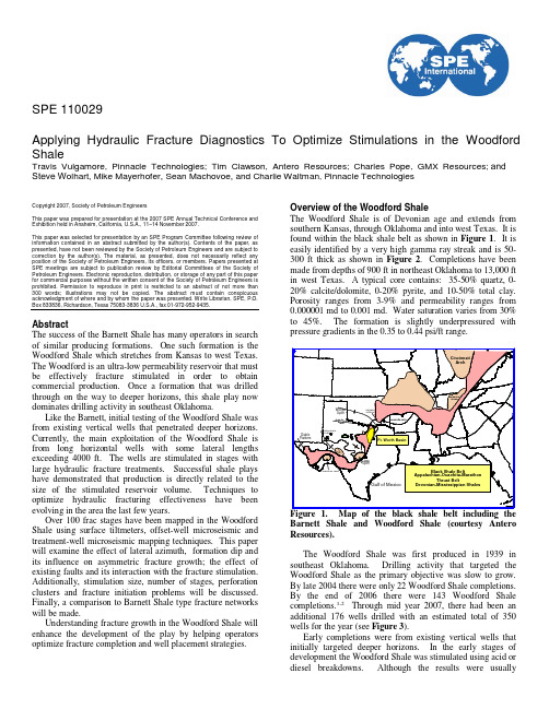
Copyright 2007, Society of Petroleum EngineersThis paper was prepared for presentation at the 2007 SPE Annual Technical Conference and Exhibition held in Anaheim, California, U.S.A., 11–14 November 2007.This paper was selected for presentation by an SPE Program Committee following review of information contained in an abstract submitted by the author(s). Contents of the paper, as presented, have not been reviewed by the Society of Petroleum Engineers and are subject to correction by the author(s). The material, as presented, does not necessarily reflect any position of the Society of Petroleum Engineers, its officers, or members. Papers presented at SPE meetings are subject to publication review by Editorial Committees of the Society of Petroleum Engineers. Electronic reproduction, distribution, or storage of any part of this paper for commercial purposes without the written consent of the Society of Petroleum Engineers is prohibited. Permission to reproduce in print is restricted to an abstract of not more than 300 words; illustrations may not be copied. The abstract must contain conspicuous acknowledgment of where and by whom the paper was presented. Write Librarian, SPE, P.O. Box 833836, Richardson, Texas 75083-3836 U.S.A., fax 01-972-952-9435.AbstractThe success of the Barnett Shale has many operators in search of similar producing formations. One such formation is the Woodford Shale which stretches from Kansas to west Texas. The Woodford is an ultra-low permeability reservoir that must be effectively fracture stimulated in order to obtain commercial production. Once a formation that was drilled through on the way to deeper horizons, this shale play now dominates drilling activity in southeast Oklahoma.Like the Barnett, initial testing of the Woodford Shale was from existing vertical wells that penetrated deeper horizons. Currently, the main exploitation of the Woodford Shale is from long horizontal wells with some lateral lengths exceeding 4000 ft. The wells are stimulated in stages with large hydraulic fracture treatments. Successful shale plays have demonstrated that production is directly related to the size of the stimulated reservoir volume. Techniques to optimize hydraulic fracturing effectiveness have been evolving in the area the last few years.Over 100 frac stages have been mapped in the Woodford Shale using surface tiltmeters, offset-well microseismic and treatment-well microseismic mapping techniques. This paper will examine the effect of lateral azimuth, formation dip and its influence on asymmetric fracture growth; the effect of existing faults and its interaction with the fracture stimulation. Additionally, stimulation size, number of stages, perforation clusters and fracture initiation problems will be discussed. Finally, a comparison to Barnett Shale type fracture networks will be made.Understanding fracture growth in the Woodford Shale will enhance the development of the play by helping operators optimize fracture completion and well placement strategies. Overview of the Woodford ShaleThe Woodford Shale is of Devonian age and extends from southern Kansas, through Oklahoma and into west Texas. It is found within the black shale belt as shown in Figure 1. It is easily identified by a very high gamma ray streak and is 50-300 ft thick as shown in Figure 2. Completions have been made from depths of 900 ft in northeast Oklahoma to 13,000 ft in west Texas. A typical core contains: 35-50% quartz, 0-20% calcite/dolomite, 0-20% pyrite, and 10-50% total clay. Porosity ranges from 3-9% and permeability ranges from 0.000001 md to 0.001 md. Water saturation varies from 30% to 45%. The formation is slightly underpressured with pressure gradients in the 0.35 to 0.44 psi/ft range.Barnett Shale and Woodford Shale (courtesy Antero Resources).The Woodford Shale was first produced in 1939 in southeast Oklahoma. Drilling activity that targeted the Woodford Shale as the primary objective was slow to grow. By late 2004 there were only 22 Woodford Shale completions. By the end of 2006 there were 143 Woodford Shale completions.1-2Through mid year 2007, there had been an additional 176 wells drilled with an estimated total of 350 wells for the year (see Figure 3).Early completions were from existing vertical wells that initially targeted deeper horizons. In the early stages of development the Woodford Shale was stimulated using acid or diesel breakdowns. Although the results were usuallySPE 110029Applying Hydraulic Fracture Diagnostics T o Optimize Stimulations in the Woodford ShaleTravis Vulgamore, Pinnacle Technologies; Tim Clawson, Antero Resources; Charles Pope, GMX Resources; and Steve W olhart, Mike Mayerhofer, Sean Machovoe, and Charlie Waltman, Pinnacle Technologies2 SPE 110029disappointing they did show that the Woodford Shale could produce hydrocarbons. The success of horizontal wells in the Barnett Shale quickly led to horizontal drilling as the primary method for exploiting the play.Figure 2. Type log for the Woodford Shale in Oklahoma (courtesy Baker Atlas).Completion and stimulation practices have generally mirrored Barnett slickwater techniques. Typical lateral lengths are 2,500 to 4,000 ft and the well is stimulated with three to ten frac stages. A typical stage consists of 7,000 to 17,000 bbls of slickwater per stage. The quantity of proppant ranges from 200,000 to 500,000 lbs per stage. The Woodford can be more difficult to stimulate than many other shales and excessive treating pressures can often prevent a stage from being successfully pumped. Fracture complexity issues have been addressed in the cementing program by using foam or acid soluble cements and in the completion by using 100 Mesh sand slugs and viscous gel slugs.Initial Potentials (IP) as high as 10 MMcf/d have been reported in the Woodford Shale with decline rates less than typically seen in the Barnett Shale.3Overview of Microseismic Fracture MappingThe microseismic hydraulic fracture mapping method is well known4-21and is only briefly reviewed here. Microseismic mapping was used to estimate fracture geometry (azimuth, half-lengths, stage height coverage) and to some degree fracture complexity. Microseisms are microearthquakes induced by the changes in stress and pore pressure associated with hydraulic fracturing. These microseisms are the result of shear-slippage that occurs along pre-existing planes of weakness (e.g., natural fractures) and emit seismic energy that can be detected at nearby borehole seismic receivers. Typically an array of tri-axial receivers in an offset well is positioned at reservoir depth near the treatment well. The microseisms produce compressional (primary or p) and shear (secondary or s) waves that are detected and analyzed in real-time to compute the locations of the events in space and time. The location of any individual event is determined from the arrival times of the p- and s-waves (provides distance and elevation) and from particle motion of the p-wave (provides azimuth from the receiver array to the event).Project 1 SettingProject 1 consisted of two vertical microseismic arrays mapping one horizontal well treated in three stages. Stages 1 and 2 were mapped using a single array in Observation Well #1 while the stage 2 refrac and stage 3 were mapped with an additional microseismic array in Observation Well #2 as well as Observation Well #1. High treating pressures during stage 2 did not allow the full treatment to be pumped during the initial attempt. The well was flowed back, then reporforated in the same intervals, before attempting a refrac. Stage 2 refrac and Stage 3 were treated 45 days following the stage 2 treatment. Figure 4 shows the location map of the three wells and the respective distance from observation well to stage perforations.SPE 110029 3Fracture treatments in this well were waterfracs. Stage volumes ranged from 17,000 bbls to 28,000 bbls of slickwater. Total proppant volumes ranged from 69,000 lbs to 430,000 lbs of 30/70 mesh Jordan sand and 60,000 lbs to 140,000 lbs of 20/40 mesh Jordan sand. Average pump rates were 85 bpm.Examples of Fracture Treatment Data for Project 1The following are examples of treatment data from stage 2 and stage 3. Stage 2 had significant treatment problems due to high treating pressures, whereas stage 3 was almost pumped to completion.Stage 2 formation breakdown was observed at 5,560psi. Following the breakdown the pump rate was decreased to 12 bpm to pump acid. The acid was flushed through the perforations before shutting down to obtain an Instantaneous Shut-In Pressure (ISIP) and fracture gradient. The fracture gradient was 0.71 psi/ft. Following the shut-in, the rate was increased to 60 bpm with a surface treating pressure of 7,100 psi. Several sand slugs were pump at concentrations between 0.1 and 0.25 ppg. As pressure dropped, rate was increased to a maximum rate of 78 bpm. The surface treating pressure began a steady increase. Rate was decreased to control the pressure but the pressure increase remained consistent reaching a maximum of 8,500 psi. The treatment was shutdown to evaluate the situation and monitor pressure decline. The fracture gradient was 0.67 psi/ft. Additional pumping was attempted with little effect. As discussed earlier, stage 2 was subsequently reperforated and refractured. Figure 5 shows the stage 2 treatment data.The stage 3 treatment started with an initial rate and pressure of 94 bpm and 8,283 psi, respectively. Several sand slugs were pumped to alleviate any friction and lower the treating pressure. The first 40/70-Mesh sand stage began with a concentration of 0.10 ppg. The 40/70-mesh sand was stepped up to a concentration of 1.00 ppg. The initial treating pressure was relatively high but quickly dropped with the addition of 40/70 sand. Following the 1.0 ppg 40/70 sand stage the 20/40-mesh sand was started at 0.40 ppg. The 20/40 sand was stepped up to 0.60 ppg where a significant increase in pressure was noted. With the pressure increasing the sand was cut and the well was flushed. The treatment ended with a final fracture gradient 0.61 psi/ft. The treatment consisted of 17,262 bbls of 2% KCl water. A total of 239,102 lbs of 40/70 sand and 59,902 lbs of 20/40 sand were pumped into formation. The average rate and surface treating pressure were 93 bpm and 6,636 psi, respectively. Figure 6 shows the stage 3 treatment data.Microseismic Mapping Results for Project 1Figure 7 shows the composite map view of the microseismic events for all three stages plus the refrac in Project 1. Fracture growth was very complex. The principal fracture network azimuth appeared to be N57°E, with significant orthogonal components generating a “wide” fracture network. Unfortunately, the beginning of Stage 1 was not monitored asCarr Estates 13- 1H Tool ArrayPettigrew 18 1H Treatment wellPettigrew 191H Tool Array2,7002,8002,6003,5002,6001,500Obs. Well #1- Treatment well Obs Well #2 -’’’’’’Figure 4. Plan view of the Project 1 project layout.4 SPE 110029wellbore preparation was behind schedule, however a large number of microseisms 2500 ft from the lateral were recorded late in the treatment. Stage 2 initiated near the perforations and produced a smaller fracture network, however it eventually extended back into the area previously stimulated during Stage 1. The large number of events tightly clustered in this area suggests the presence of a fault(s) or naturally-fractured reservoir. The linear character of stage two events (crossing Observation well #1) suggests intersection with a previously stimulated). The Stage 2 refrac was mapped 45 days later and it appeared to have fracture half-lengths of about 1,500 ft. As in previous stages, the treatment grew asymmetrically up-dip (to the west). This was confirmed by Observation well #2 which was in a better location to determine asymmetry. Interestingly no microseisms were located in the previously stimulated area northeast of Observation well #1. Stage 3 treatment produced a small fracture network near the perforations. Numerous events were also located far from the lateral and very close to Observation well #1. Overall fracture network lengths varied from about 1,200 ft to 3,300 ft and also grew asymmetrically up-dip to the west.Figure 8 and Figure 9 show the side view and edge view of all mapped stages for Project 1. Fracture heights ranged from about 250 ft to 280 ft with the majority of the events contained within and following the dip of the Woodford shale westwards towards Observation Well #1.Carr Estate 13-1HPettigrew 18-1H Woodford-@ frac wellPettigrew 19-1HObs Well #1- Treatment WellUp -dip @Obs. wellWoodford-Obs Well #2- Looking NEStimulated reservoir volume (SRV) can be calculated the product of fracture network area and stimulated pay thickness. In Project 1 the SRV is about 1,274 (106 ft 3) 29,247 acre-ft, which is comparable to SRV’s measured in the Barnett shale. This indicates that interaction with natural fractures and faults can create similar size networks in the Woodford shale. Carr Estate 13-1H Pettigrew 18-1HWoodfordPettigrew 19-1H Obs Well #1Treatment Well FMObs Well #2Stage 2 events Stage 1 events Stage 2RF events Stage 3 eventsLooking NWObs Well #1Project 2 SettingProject 2 included a single horizontal well which was mapped with a single microseismic array from two locations. Stage 1 was mapped from Observation Well #1 and stages 2 to 6 were mapped from Observation Well #2. The treatment well wasPettigrew 19N57Carr Estates 131HTool Array 1H Tool ArrayPettigrew 181HTreatment wellObs Well #1 -- Obs Well #2- Treatment wellStage 1 Stage 2Stage 2 RF Stage 3°EFigure 7. Plan view showing microseismic mapping results for Project 1. Figure 8. Side view showing microseismic events for all stages mapped in Project 1. Figure 9. Edge view of microseismic events for all mappedSPE 110029 5drilled from north to south (updip). Figure 10 shows the location map of the Project 1 treatment well and observation wells. Treatment 3,600’3,400’2,500’2,000’800’1,200’1,450’Obs Well #2Obs Well #1WellThe well was stimulated with six fracture treatment stages. Mapping distances ranged from 800 ft to 3,600 ft depending on stage and observation well location. Fracture treatments were pumped using treated water ranging from 7,000 bbls to 16,500 bbls of fluid. Total proppant volumes ranged from 50,000 lbs to 225,000 lbs of 30/70 mesh Jordan sand and 35,000 lbs to 78,000 lbs of 20/40 mesh Jordan sand.Microseismic Mapping Results for Project 2Figure 11 shows the composite map view of the microseismic events for all six stages mapped in Project 2. Fracture network azimuth varies from about N60°E to N90°E. Stages 5 and 6 appeared to intersect a fault(s) or heavily naturally-fractured area west of the lateral. Toward the end of stage 5 numerous larger magnitude events began to appear in a cluster 800 ft away from the fracturing near the perforations. These events continued to occur well after the termination of the treatment. This phenomenon had been observed in other areas and was a good indication of interaction with faulting or other structural deformation. The Stage 6 treatment initiated at the perforations but quickly grew southwest towards the cluster of events observed during Stage 5.Treatment N90°EN90°EN90°E N110°EN90°E N70°EN60°E Obs Well #2WellFigure 11. Plan view showing microseismic mapping results for Project 2.Created fracture network lengths ranged from 400 ft to 1,350 ft. The created fracture networks were generally symmetric about the wellbore. However, Stages 5 and 6 appeared to be more asymmetrical because of the interaction with the area of structural deformation west of the lateral. Figure 12 shows a side view of all microseismic events associated with Project 2. Fracture heights ranged from 110 ft to 300 ft and treatments appear to be mostly contained within the Woodford. Fracture height was very difficult to determine during Stages 1 and 2 because of the large observation distance (more than 3,000 ft) and small magnitude microseisms. It was not possible to calculate a precise SRV for this project.Figure 10. Plan view showing the location of wells for Project 2.6 SPE 110029Treatment T o p o fW o o dfo r d S ha leWellTool ArrayFigure 12. Side view showing mapping results for Project 2.Project 3 SettingProject 3 included a single horizontal well which was mapped with a single microseismic array. The treatment well was drilled from south to north (downdip) and the tool array was placed in the vertical section of an offset horizontal well. Figure 13 shows the location map of the Project 3 treatment well and observation well. Observation Treatment wellWell2,800’3,000’3,400’3,800’4,300’The horizontal well was stimulated with five fracture treatment stages. Mapping distances ranged from 2,800 ft at the toe to 4,300 ft at the heel. Fracture treatments werepumped using treated water ranging from 10,000 bbls to 20,000 bbls of fluid. Total proppant volumes amounts ranged from 32,000 lbs to 100,000 lbs of 30/70 mesh Jordan sand and 58,000 lbs to 222,000 lbs of 20/40 mesh Jordan sand and 100-mesh sand was also used as a diverting agent.Microseismic Mapping Results for Project 3Figure 14 shows the composite map view of the microseismic events for all five stages monitored in Project 3. The dominant fracture network azimuth appeared to be N60°E, with a secondary NW-SE orthogonal component. Fracture half-lengths were very long, ranging from at least 1,360 ft to 3,300 ft. Fracture geometry from Stages 1 to 3 was complex, but well-defined as the treatments grew directly towards the microseismic toolstring. Stages 2, 3, and 5 appeared to intersect the observation well. Most of the stages had overlapping fracture networks with network widths ranging from 900 ft to 2,000 ft. Fracture heights ranged from about 250 ft to 350 ft and were mostly contained in the Woodford shale (Figure 15). 100-mesh sand was added to the pad in Stage 3 to divert fluid from the linear fault-like feature in Stage 2, which resulted in a change of fracture pattern. Stages 4 and 5 were much farther from the microseismic toolstring and fewer events were recorded due to signal attenuation; however enough of the larger events were recorded to define fracture azimuth and half-lengths. Overall signal quality was very good, and events up to 5,000 ft away were imaged, including some very large magnitude events near the lateral (Figure 16).SRV could not be precisely calculated for this well, since stages 4 and 5 were not fully mapped. However, qualitatively the SRV would fall in the upper half of Barnett shale SRV’s. Observation Stage 1Stage 2Stage 3Stage 4Stage 5WellTreatment wellFigure 14. Plan view showing microseismic mapping results for Project 3.Figure 13. Plan view showing the location of wells for Project 3.SPE 110029 7Figure 15. Side view showing microseismic mapping results for Project 3.Figure 16. Magnitude versus distance plot for microseismic events from Project 3.ProductionA correlation has been found between SRV and well performance in the Barnett Shale.22-24 Sufficient SRV and production data is not yet available in order to develop a similar correlation for the Woodford Shale. Only Project 1 in this paper had sufficient microseismic information on all stages to warrant a SRV calculation. Figure 17 shows a cumulative frequency plot of Barnett core area SRV’s versus Project 1 SRV. It shows that the SRV for Project 1 would fall in the upper half of Barnett SRV’s.diagnostics results:1. Fracture treatments in the Woodford shale generatecomplex fracture networks with multiple fracture orientations similar to the Barnett shale. The primary fracture network azimuth appears to N60-70o E with variations ranging from N45o E to N90o E. A significant orthogonal component giving fracture networks significant “width” was observed.2. The interaction with local structural features (faults,fracture swarms) had a significant effect on fracture treatment geometry. They can completely dominate fracture growth as subsequent stages may continue to grow into the previously intersected fault. This can prevent the full length of the lateral from being stimulated and may cause the well to underperform. 3. Observed fracture network dimensions arecomparable to the Barnett Shale but more interaction with geologic features appears to be present in the Woodford shale.4. Asymmetric fracture growth was observed in severaltreatments. Fracture networks had the tendency to grow up dip.5. Fracture network half-lengths up to 3,300 feet havebeen observed. A single stage will have a network width of about 300 to 500 ft along the lateral. Small perforation clusters perform better and have less fracture entry problems. When injectivity is limited, 100-mesh sand slugs or small crosslink-gel slugs help eliminate near wellbore complexities.SummaryMost early Woodford completion and stimulation designs were modeled according to Barnett principles. The operator used, and continues to use, microseismic mapping to evaluate the effectiveness of those, and subsequent, practices. Lessons learned to date have led to better results via changes made in: stage lengths, cluster number/spacing per stage, fluid/sand8 SPE 110029volumes per foot of lateral, pump rate, proppant type/concentration and simultaneous well stimulations. AcknowledgementsThe authors would like to thank Antero Resources for permission to publish this work and John Alcott and Ulrich Zimmer with Pinnacle Technologies for additional microseismic analysis and interpretation.References1. Brian J. Cardott: “Overview of the Woodford Gas Shale Play inOklahoma,” presented at the Woodford Gas Shale Conference,Oklahoma City, Oklahoma, 23 May 2007,(/pdf/WoodfordOverview.pdf).2.Haines, L., “Activity Builds in Woodford Shale,” supplement toOil and Gas Investor, January 2006 (17).3.Boothby, L.K.: “Newfield Provides Update on Woodford ShalePlay,” presented at the Bank of America Energy Conference, Key Biscayne, Florida, 17 November 2006.4.Rocky Stewart, L., Cassell, B.R. and Bol, G.M., "Acoustic-Emission Monitoring During Hydraulic Fracturing," SPE Formation Evaluation, Vol. 7, pp. 139-144, June 1992.5.Pearson, C., "The Relationship between Microseismicity andHigh Pore Pressures during Hydraulic Stimulation Experiments in Low Permeability Granitic Rocks," J.Geophys. Res., Vol. 86, pp. 7855-7864, September 1981.6.Fehler, M.C., "Stress Control of Seismicity Patterns ObservedDuring Hydraulic Fracturing Experiments at the Fenton Hill Hot Dry Rock Geothermal Energy Site, New Mexico," Int. J.Rock Mech., Min. Sci. & Geomech. Abstr., Vol. 26, pp. 211-219, 1989.7.Peterson, R.E., Wolhart, S.L., Frohne, K.-H., Warpinski, N.R.,Branagan, P.T. and Wright, T.B., “Fracture Diagnostics Research at the GRI/DOE Multi-Site Project: Overview of the Concept and Results,” SPE 36449, SPE Annual Technical Conference & Exhibition, Denver, CO, October 6-9, 1996.8.Warpinski, N.R., Wright, T.B., Uhl, J.E., Engler, B.P., Drozda,P.M. and Peterson, R.E., “Microseismic Monitoring of the B-Sand Hydraulic Fracture Experiment at the DOE/GRI Multi-Site Project,” SPE 36450, SPE Annual Technical Conference & Exhibition, Denver, CO, October 6-9, 1996.9.Sleefe, G.E., Warpinski, N.R. and Engler, B.P., “The Use ofBroadband Microseisms for Hydraulic Fracture Mapping,”SPE Formation Evaluation, pp. 233-239, Dec. 1995.10.Warpinski, N.R., Engler, B.P., Young, C.J., Peterson, R.,Branagan, P.T. and Fix, J.E., “Microseismic Mapping of Hydraulic Fractures Using Multi-Level Wireline Receivers,”SPE 30507, SPE Annual Technical Conference & Exhibition, Dallas, TX, Oct. 22-25, pp. 579-589, 1995.11.Warpinski, N.R., Branagan, P.T., Peterson, R.E., Fix, J.E., Uhl,J.E., Engler, B.P. and Wilmer, R., “Microseismic and Deformation Imaging of Hydraulic Fracture Growth and Geometry in the C Sand Interval, GRI/DOE M-Site Project,”SPE 38573, SPE Annual Technical Conference & Exhibition, San Antonio, TX, October 5-8, 1997.12.Warpinski, N.R., Branagan, P.T., Peterson, R.E., Wolhart, S.L.and Uhl, J.E., “Mapping Hydraulic Fracture Growth and Geometry Using Microseismic Events Detected by a Wireline Retrievable Accelerometer Array,” SPE 40014, 1998 Gas Technology Symposium, Calgary, Alberta, Canada, March 15-18.13.Warpinski, N.R., Branagan, P.T., Peterson, R.E., and Wolhart,S.L., “An Interpretation of M-Site Hydraulic Fracture Diagnostic Results,” SPE 39950, Rocky MountainRegional/Low Permeability Reservoirs Symposium and Exhibition, Denver, CO., pp. 407-420, 1998.14.Phillips, W.S., Fairbanks, T.D., Rutledge, J.T., and Anderson,D.W., “Induced Microearthquake Patterns and Oil-ProducingFracture Systems in the Austin Chalk,” Tectonophysics, Vol.289, pp. 153-169, 1998.15.Talebi, S., Young, R.P., Vandamme, L. and McGaughey, W.J.,“Microseismic Mapping of a Hydraulic Fracture,” Proc. 32nd US Symposium on Rock Mechanics, University of Oklahoma, Norman, OK, pp. 461-470, 1991.16.Vandamme, L., Talebi, S. and Young, R.P., “Monitoring of aHydraulic Fracture in a South Saskatchewan Oil Field,”Journal of Canadian Petroleum Technology, Vol. 33, No. 1, pp. 27-33, January 1994.17.Withers, R.J., Perkins, T.K. and Keck, R.G., “A FieldDemonstration of Hydraulic Fracturing for Solids Waste Disposal, Part Two: Real Time Passive Seismic Monitoring System and Data Analysis,” in Deep Injection Disposal of Hazardous and Industrial Waste, J.A. Apps and C.F. Tsang, eds., Academic Press, pp. 705-724, San Diego, 1996.18. Brady, J.L., Withers, R.J., Fairbanks, T.D. and Dressen, D.,“Microseismic Monitoring of Hydraulic Fractures in Prudhoe Bay, SPE 28553, 69th SPE Annual Technical Conference & Exhibition, Vol. Π, pp. 387-398, New Orleans, LA, Sept. 25-28, 1994.19.Warpinski, N.R., Branagan, P.T., Wolhart, S.L., Moschovidis,Z.A. and Mahrer, K.D., “Microseismic Monitoring of the Mounds Drill Cuttings Injection Tests,” Proc., 37th U.S. Rock Mechanics Symposium, Vail Colorado, pp. 1025-1032, June 6-9, 1999.20.Warpinski, N. R., Wolhart, S. L, and Wright, C. A., “Analysisand Prediction of Microseismicity Induced by Hydraulic Fracturing,” SPE 71649, SPE Annual Technical Conference & Exhibition, New Orleans, LA, Sept 30 –October 3, 2001.21.Warpinski, N.R, Sullivan, R.B, Uhl, J.E.., Waltman, C.K., andMachovoe, S.R., “Improved Microseismic Fracture Mapping Using Perforation Timing Measurements for Velocity Calibration,” SPE 84488, SPE Annual Technical Conference & Exhibition, Denver, Colorado, October 5 – 8, 2003.22.Fisher, M.K., Davidson, B.M., Goodwin, A.K., Fielder, E.O.,Buckler, W.S. and Steinberger, N.P.: “Integrating Fracture Mapping Technologies to Optimize Stimulations in the Barnett Shale,” paper SPE 77411 presented at the 2002 SPE Annual Technical Conference and Exhibition, San Antonio, Texas, 29 September–2 October.23.Fisher, M.K., Heinze, J.R., Harris, C.D, Davidson, B.M.,Wright, C.A., and Dunn, K.P.: “Optimizing Horizontal Completion Techniques in the Barnett Shale Using Microseismic Fracture Mapping,” paper SPE 90051 presented at the 2004 SPE Annual Technical Conference and Exhibition, Houston, Texas, 27–29 September.24.Mayerhofer, M.J., Lolon, E.P., Youngblood, J.E., Heinze, J.R.:”Integration of Microseismic Fracture Mapping Results with Numerical Fracture Network Production Modeling in the Barnett Shale”, SPE 102103 presented at the 2006 SPE Annual Technical Conference and Exhibition held in San Antonio, Texas, U.S.A., 24–27 September 2006.。

微带耦合器的中英文对照翻译

微带耦合器的中英文对照翻译Design and Analysis of Wideband Nonuniform Branch Line Coupler and Its Application in a Wideband Butler MatrixYuli K. Ningsih,1,2 M. Asvial,1 and E. T. RahardjoAntenna Propagation and Microwave Research Group (AMRG), Department of Electrical Engineering, Universitas Indonesia, New Campus UI, West Java, Depok 16424, Indonesia Department of Electrical Engineering, Trisakti University, Kyai Tapa, Grogol, West Jakarta 11440, IndonesiaReceived 10 August 2011; Accepted 2 December 2011Academic Editor: Tayeb A. DenwdnyCopyright ? 2012 Yuli K. Ningsih et al. This is an open access article distributed under the Creative Commons Attribution License, which permits unrestricted use, distribution, and reproduction in any medium, provided the original work is properly cited.AbstractThis paper presents a novel wideband nonuniform branch line coupler. An exponential impedance taper is inserted, at the series arms of the branch line coupler, to enhance the bandwidth. The behavior of the nonuniform coupler was mathematically analyzed, and its design of scattering matrix was derived. For a return loss better than 10?dB, itachieved 61.1% bandwidth centered at 9GHz. Measured coupling magnitudes and phase exhibit good dispersive characteristic. For the 1dB magnitude difference and phase error within 3°, it achieved 22.2% bandwidth centered at 9GHz. Furthermore, the novel branch line coupler was implemented for a wideband crossover. Crossover was constructed by cascading two wideband nonuniform branch line couplers. These components were employed to design a wideband Butler Matrix working at 9.4GHz. The measurement results show that the reflection coefficient between the output ports is better than 18dB across 8.0GHz–9.6GHz, and the overall phase error is less than 7.1. IntroductionRecently, a switched-beam antenna system has been widely used in numerous applications, such as in mobile communication system, satellite system, and modern multifunction radar. This is due to the ability of the switched-beam antenna to decrease the interference and to improve the quality of transmission and also to increase gain and diversity.The switched-beam system consists of a multibeam switching network and antenna array. The principle of a switched-beam is based on feeding a signal into an array of antenna with equal power and phase difference. Different structures of multibeam switching networks have been proposed, such as the Blass Matrix, the Nolen Matrix, the RotmanLens, and the Butler Matrix .One of the most widely known multibeam switching networks with a linear antenna is the Butler Matrix. Indeed, it seems to be the most attractive option due to its design simplicity and low power loss .In general, the Butler Matrix is an N × N passive feeding network, composed of branch line coupler, crossover, and phase shifter. The bandwidth of the Butler Matrix is greatly dependent on the performance of the components. However, the Butler Matrix has a narrow bandwidth characteristic due to branch line coupler and crossover has a limited bandwidth. As there is an increased demand to provide high data throughput , it is essential that the Butler Matrix has to operate over a wide frequency band when used for angle diversity. Therefore, many papers have reported for the bandwidth enhancement of branch line coupler . In reference , design and realization of branch line coupler on multilayer microstrip structure was reported. These designs can achieve a wideband characteristic. However, the disadvantages of these designs are large in dimension and bulk.Reference introduces a compact coupler in an N-sectiontandem-connected structure. The design resulted in a wide bandwidth. Another design, two elliptically shaped microstrip lines which are broadside coupled through an elliptically shaped slot, was employed in . This design was used in a UWB coupler with high return loss andisolation. However, these designs require a more complex manufacturing.In this paper, nonuniform branch line coupler using exponential impedance taper is proposed which can enhance bandwidth and can be implemented for Butler Matrix, as shown in Figure1. Moreover, it is a simple design without needs of using multilayer technology. This will lead in cost reduction and in design simplification.Figure 1:Geometry structure of a new nonuniform branch line coupler design with exponential impedance taper at the series arm.To design the new branch line coupler, firstly, the series arm’s impedance is modified. The shunt arm remains unchanged. Reduced of the width of the transmission line at this arm is desired by modifying the series arm. Next, by exponential impedance taper at the series arm, a good match over a high frequency can be achieved.2. Mathematical Analysis of Nonuniform Branch Line CouplerThe proposed nonuniform branch line coupler use λ/4 branches with impedance of 50Ω at the shunt arms and use the exponential impedance taper at the series arms, as shown in Figure1. Since branch line coupler has a symmetric structure, theeven-odd mode theory can be employed to analyze the nonuniform characteristics. The four ports can be simplified to a two-port problem in which the even and odd mode signals are fed to two collinear inputs [22].Figure 2 shows the schematic of circuit the nonuniform branch line coupiers.Figure 2:Circuit of the nonuniform branch line coupler.The circuit of Figure 2 can be decomposed into the superposition of an even-mode excitation and an odd-mode excitation is shown in Figures and .Figure 3:Decomposition of the nonuniform branch line coupler into even and odd modes of excitation.The ABCD matrices of each mode can be expressed following . In the case of nonuniform branch line coupler, the matrices for the even and odd modes become:A branch line coupler has been designed based on the theory of small reflection, by the continuously tapered line with exponential tapers , as indicated in Figure 1, wherewhich determines the constant as:Useful conversions for two-port network parameters for the even and odd modes of S11 and S21 can be defined as follows :whereSince the amplitude of the incident waves for these two ports are ±1/2, the amplitudes of the emerging wave at each port of the nonuniform branch line coupler can be expressed asParameters even and odd modes of S11 nonuniform branch linecoupler can be expressed as and as follows:An ideal branch line coupler is designedto have zero reflection power and splits the input power in port 1 (P1) into equal powers in port 3 (P3) and port 4 (P4). Considering to , a number of properties of the ideal branch line coupler maybe deduced from the symmetry and unitary properties of its scattering matrix. If the series and shunt arm are one-quarter wavelength, by using , resulted in S11 = 0.As both the even and odd modes of S11 are 0, the values of S11 and S21 are also 0. The magnitude of the signal at the coupled port is then the same as that of the input port.Calculating and under the same , the even and odd modes ofS21 nonuniform branch line coupler will be expressed as follows in Based on ,S11 can be expressed as follows Following ,S41 nonuniform branch line coupler can be calculating as followsFrom this result, both S31 and S41 nonuniform branch line couplers have equal magnitudes of ?3dB. Therefore, due to symmetry property, we also have thatS11=S22=S33=S44=0,S13=S31，S14=S41，S21=S34, and . Therefore, the nonuniform branch line coupler has the following scattering matrix in3. Fabrication and Measurement Result of Wideband Nonuniform Branch Line CouplerTo verify the equation, the nonuniform branch line coupler was implemented and its -parameter was measured. It was integrated on TLY substrate, which has a thickness of 1.57mm. Figure 4 shows a photograph of a wideband nonuniform branch line coupler. Each branch at the series arm comprises an exponentially tapered microstrip line which transforms the impedance from ohms to ohms. This impedance transformation has been designed across a discrete step length mm.Figure 4:Photograph of a proposed nonuniform branch line coupler.Figure 5 shows the measured result frequency response of the novel nonuniform branch line coupler. For a return loss and isolation better than 10dB, it has a bandwidth of about 61.1%; it extends from 7 to 12.5GHz. In this bandwidth, the coupling ratio varies between 2.6?dB up to 5.1dB. If the coupling ratio is supposed approximately 3 ± 1dB, the bandwidth of about 22.2% centered at 9GHz.Figure 5:Measurement result for nonuniform branch line coupler.As expected, the phase difference between port 3 (P3) and port 4 (P4) is 90°. At 9?GHz, the phases of and are 85.54° and 171°, respectively. These values differ from ideal value by4.54°. The average phase error or phase unbalance between two branch line coupler outputs is about 3°. But even the phase varies with frequency; the phase difference is almost constant and very close toideal value of 90° as shown in Figure 6.Figure 6:Phase characteristic of nonuniform branch line coupler.4. Design and Fabrication of the Wideband Butler MatrixFigure 7 shows the basic schematic of the Butler Matrix . Crossover also known as 0dB couplers is a four-port device and must provide for a very good matching and isolation, while the transmitted signal should not be affected. In order to achieve wideband characteristic crossover, this paper proposes the cascade of two nonuniform branch line couplers.Figure 7:Basic schematic of the Butler Matrix .Figure 8 shows the microstrip layout of the optimized crossover. The crossover has a frequency bandwidth of 1.3GHz with VSWR = 2, which is about 22.2% of its centre frequency at 9?GHz. Thus, it is clear from these results that a nonuniform crossover fulfills most of the required specifications, as shown in Figure 9.Figure 8:Photograph of microstrip nonuniform crossover.Figure 9:Measurement result for nonuniform crossover.Figure 10 shows the layout of the proposed wideband Butler Matrix. This matrix uses wideband nonuniform branch line coupler, wideband nonuniform crossover, and phase-shift transmission lines.Figure 10:Final layout of the proposed wideband Butler Matrix .The wideband Butler Matrix was measured using Network Analyzer.Figure 11 shows thesimulation and measurement results of insertion loss when a signal was fed into port 1, port 2, port 3, and port 4, respectively. The insertion loss are varies between 5dB up to 10dB. For the ideal Butler matrix, it should be better than 6dB. Imperfection of fabrication could contribute to reduction of the insertion loss.Figure 11:Insertion loss of the proposed Butler Matrix when different ports are fed. The simulated and measured results of the return loss at each port of the widedend Butler Matrix is shown in Figure 12. For a return loss better than 10dB, it has a bandwidth about 17% centered at 9.4GHz.Figure 12:Return loss of the proposed Butler Matrix when different ports are fed.Figure 13 shows the phase difference of measured results when a signal was fed into port 1, port 2, port 3, and port 4, respectively. The overall phase error was less than 7°. There are several possible reasons for this phase error. A lot of bends in high frequency can produce phase error. Moreover, the imperfection of soldering, etching, alignment, and fastening also could contribute to deviation of the phase error.Figure 13:Phase difference of the proposed Butler Matrix when different ports are fed. Table 1 shows that each input port was resulted a specific linear phase at the output ports. The phase differences eachbetween the output ports are of the same value. The phase difference can generate a different beam ( θ). If port 1 (P1) is excited, the phase difference was 45°, the direction of generated beam ( θ) will be 14.4° for 1L. It is summarized in Table 1.Table 1:Output phase difference and estimated direction of generated beam.5. ConclusionA novel nonuniform branch line coupler has been employed to achieve a wideband characteristic by exponential impedance taper technique. It is a simple design without needs of using multilayer technology and this will lead to cost reduction and design simplification. The scattering matrix of the nonuniform branch line coupler was derived and it was proved that the nonuniform branch line coupler has equal magnitude of ?3dB. Moreover, the novel nonuniform branch line coupler has been employed to achieve a wideband 0dB crossover. Furthermore, these components have been implemented in the Butler Matrix and that achieves wideband characteristics.References? T. A. Denidni and T. E. Libar, “Wide band four-port butler matrix for switched multibeam antenna array s,” in Proceedings of the IEEE International Symposium on Personal, Indoor and Mobile Radio Communications (PIMRC '03), vol. 3, pp. 2461–2464, 2003. View atPublisher ·View at Google Scholar? E. Siachalou, E. Vafiadis, S. S. Goudos, T. Samaras, C. S. Koukourlis, and S. Panas, “On the design of switched-beam wideband base stations,” IEEE Antennas and Propagation Magazine, vol. 46, no. 1, pp. 158–167, 2004. View at Publisher ·View at Google Scholar ·View at Scopus ? P. S. Hall and S. J. Vetterlei n, “Review of radio frequency beamforming techniques for scanned and multiple beam antennas,” IEE Proceedings H, vol. 137, no. 5, pp. 293–303, 1990. View at Scopus ?? W-D. Wirth, Radar Techniques Using Array Anney, IEE Publishers, Stevenage, UK, 2001. S. Y. Zheng, S. H. Yeung, W. S. Chan, and K. F. Man, “Broadband butler matrix optimized using jumping genes evolutionary algorithm,” in Proceedings of the IEEE International Conference on Industrial Technology (IEEE ICIT '08), Hong Kong, April 2008. Viewat Publisher ·View at Google Scholar? K. Wincza and K. Sachse, “Broadband Butler matrix in microstrip multilayer technology designed with the use of three-section directional couplers and phase correction Networks,” in Proceedings of the 18th International Conference on Microwave Radar and Wireless Communications(MIKON '10), Cracow, Poland, June 2010.? A. M. El Tager and M. A. Eleiwa, “Design and implementation of a smart antenna using butler matrix for ISM band,” in Proceedings of th eProgress in Electromagnetics Research Symposium (PIERS '09), pp. 571–575, Beijing, China, March 2009.? Y. S. Jeong and T. W. Kim, “Design and analysis of swapped port coupler and its application in a miniaturized butler matrix,” IEEE Transactions on Microwave Theory and Techniques, vol. 58, no. 4, pp. 764–770, 2010. View at Publisher ·View at Google Scholar ·View at Scopus? C. Collado, A. Grau, and F. De Flaviis, “Dual-band butler matrix for WLAN systems,” in IEEE MTT-S International Microwave Symposium Digest, vol. 2005, pp. 2247–2250, 2009. View at Publisher ·View at Google Scholar?? K. Wincza, S. Gruszczynski, and K. Sachse, “Integrated four-beam dual-band antenna array fed by broadband Butler matrix,” Electronics Letters, vol. 43, no. 1, pp. 7–8, 2007. View at Publisher ·View at Google Scholar ·View at Scopus?? T. N. Kaifas and J. N. Sahalos, “On the design of a single-layer wideband Butler matrix for switched-beam UMTS system applications,” IEEE Antennas and Propagation Magazine, vol. 48, no. 6, pp. 193–204, 2006. View at Publisher ·View at Google Scholar ·View at Scopus ?? K. Wincza and S. Gruszczynski, “A broadband 4 × 4 butler matrix for modern-day antennas,” in Proceedings of the 35th European Microwave Conference, pp. 1331–1334, Paris, France, October 2005.View at Publisher ·View at Google Scholar?? S. Gruszczyoski, K. Wincza, and K. Sachse, “Reduced sidelobefour-beam N-element antenna arrays fed by 4 × 4 N butler matrices,” IEEE Antennas and Wireless PropagationLetters, vol. 5, no. 1, pp. 430–434, 2006. View at Publisher ·View at Google Scholar ·View at Scopus?? Y. C. Su, M. E. Bialkowski, F. C. E. Tsai, and K. H. Cheng, “UWB switched-beam array antenna employing UWB butler matrix,” in Proceedings of the IEEE International Workshop on Antenna Technology: Small Antennas and Novel Metamaterials (iWAT '08), pp. 199–202, Hsinchu, Taiwan, March 2008. View at Publisher ·View at Google Scholar ?? J. He, B. Z. Wang, Q. Q. He, Y. X. Xing, and Z. L. Yin, “Wi debandx-band microstrip Butler matrix,” Progress in Electromagnetics Research, vol. 74, pp. 131–140, 2007. View at Scopus?? Y. Liuqing and G. B. Giannakis, “Ultra wideband communications,” IEEE Signal Processing Magazine, vol. 21, no. 6, pp. 26–54, 2004. View at Publisher ·View at Google Scholar ·View at Scopus?? S. Banba and H. Ogawa, “Multilayer MMIC directional c ouplers using thin dielectric layers,” IEEE Transactions on Microwave Theory and Techniques, vol. 43, no. 6, pp. 1270–1275, 1995. View at Publisher ·View at Google Scholar ·View at Scopus?? J. Sebastien and G. Y. Delisle, “Microstrip EHF butler matrixdesign and realization,” ETRI Journal, vol. 27, no. 6, pp. 788–797, 2005. View at Scopus?? J. H. Cho, H. Y. Hwang, and S. W. Yun, “A design of wideband 3-dB coupler with N-section microstrip tandem structure,” IEEE Microwave and Wireless Components Letters, vol. 15, no. 2, pp. 113–115, 2005. View at Publisher ·View at Google Scholar ·View at Scopus ?? M. E. Bialkowski, N. Seman, and M. S. Leong, “Design of a compact ultra wideband 3? db microstrip-slot coupler with high return losses and isolation,” i n Asia Pacific Microwave Conference (APMC '09), pp. 1334–1337, St. Lucia, Australia, December 2009. View at Publisher ·View at Google Scholar?? R. P. Hecken, “A near-optimum matching section without discontinuities,” IEEETransactions on Microwave Theory and Techniques, vol. 20, no. 11, pp. 734–739, 1972. ?? D. M. Pozar, Microwave Engineering, John Wiley& Sons, New York, NY, USA, 2nd edition, 1998.?? M. Bona, L. Manholm, J. P. Starski, and B. Svensson, “Low loss compact butler matrix for a microstrip antenna,” IEEE Transactions on Microwave Theory and Techniques, vol. 50, no. 9, pp. 2069–2075, 2002. View at Publisher ·View at Google Scholar?? M. Kobayashi and N. Sawada, “Analysis and synthesis of tapered microstriptransmissio n lines,” IEEE Transactions on Microwave Theory and Techniques, vol. 40, no. 8, pp. 1642–1646, 1992. View at Publisher ·View at Google Scholar宽带非均匀支线耦合器及其应用在宽带巴特勒矩阵的设计与分析协作院校：印尼大学新校区电机工程学系天线传播和微波研究小组（AMRG）。

SiBN

第３６卷第３期２０１５年６月
ＤＯＩ：１０．１３９５７￣．ｃｎｋｉ．ｔｃｘｂ．２０１５．０３．００３
鹭李旅
ＪｏｕｒｎａｌｏｆＣｅｒａｍｉｃｓ
ＶＯ１．３６ＮＯ．３Ｊｕｎ．２０１５
ＭＡＮａ，ＭＥＮＷｅｉｗｅｉ，ＷＡＮＧＺｈｉｑｉａｎｇ，ＸＵＡＮＬｉｘｉｎ
（ＴｈｅＡｅｒｏｎａｕｔｉｃａｌＳｃｉｅｎｃｅＫｅｙＬａｂｆｏｒＨｉｇｈＰｅｒｆｏｒｍａｎｃｅＥｌｅｃｔｒｏｍａｇｎｅｔｉｃＷｉｎｄｏｗｓ，ＲｅｓｅａｒｃｈＩｎｓｔｉｔｕｔｅｏｒｆＳｐｅｃｉａｌＳｔｒｕｃｔｕｒｅｓｏｆ
ｐｒｅｄｉｃｔｅｄｉｔｓｆｕｔｕｒｅｄｅｖｅｌｏｐｍｅｎｔｓ．
Ｋｅｙｗｏｒｄｓ：ｗａｖｅ・ｔｒａｎｓｐａｒｅｎｔｍａｔｅｒｉａｌ；ｃｅｒｍｉａｃｉｆｂｅｒ；ＳｉＢＮ（Ｃ）
关键词：透波材料；陶瓷纤维；ＳｉＢＮ（Ｃ）
中图分类号：ＴＱ１７４．７５文献标志码：Ａ文章编号：１０００－２２７８（２０１５）０３－０２２７－０６
ＰｒｏｇｒｅｓｓｉｎｔｈｅＲｅｓｅａｒｃｈｏｆＳｉＢＮ（Ｃ）Ｗａｖｅ — ｔｒａｎｓｐａｒｅｎｔＣｅｒａｍｉｃＦｉｂｅｒ

G781_DataSheet

±1°C Remote and Local Temperature Sensor with SMBus Serial InterfaceFeaturesTwo Channels: Measures Both Remote andLocal Temperatures No Calibration RequiredSMBus 2-Wire Serial InterfaceProgrammable Under/Overtemperature Alarms Supports SMBus Alert Response Accuracy:±1°C (+60°C to +100°C, remote) ±3°C (+60°C to + 100°C, local)320µA (typ) Average Supply Current During Conversion+3V to +5.5V Supply Range Small 8-Lead SO PackageApplications Desktop and Notebook Central Office Computers Telecom Equipment Smart Battery Packs Test and Measurement LAN Servers Multi-Chip Modules Industrial Controllers General DescriptionThe G781 is a precise digital thermometer that reports the temperature of both a remote sensor and its own package. The remote sensor is a diode-connected transistor typically a low-cost, easily mounted 2N3904 NPN type that replace conventional thermistors or thermocouples. Remote accuracy is ±1°C with no cali-bration needed. The remote channel can also meas-ure the die temperature of other ICs, such as micro-processors, that contain an on-chip, diode-connected transistor.The 2-wire serial interface accepts standard System Management Bus (SMBus) Write Byte, Read Byte, Send Byte, and Receive Byte commands to program the alarm thresholds and to read temperature data.The data format is 11bits plus sign, with each bit cor-responding to 0.125°C, in two’s-complement format. Measurements can be done automatically and autonomously, with the conversion rate programmed by the user or programmed to operate in a single-shot mode. The adjustable rate allows the user to control the supply current drain.The G781 is available in a small, 8-pin SOP sur-face-mount package.Ordering InformationPART* TEMP. RANGE PIN-PACKAGEG781-20°C to +120°C8-SOPPin ConfigurationTypical Operating Circuit3V TO 5.5VEACHCLOCK DATAINTERRUPT TO µCSMBDATA SMBCLK GNDG781ALERTAbsolute Maximum RatingsVCC to GND………….….……..………….-0.3V to +6V DXP to GND……….……………..…-0.3V to VCC + 0.3V DXN to GND……………..……………..-0.3V to +0.8V SMBCLK, SMBDATA,ALERT to GND..…-0.3V to +6V SMBDATA,ALERT Current………….-1mA to +50mA DXN Current……………………..………………….±1mA ESD Protection (SMBCLK, SMBDATA,ALERT , humanbody model).……………………………………….2000V ESD Protection (other pins, human body model)..2000V Continuous Power Dissipation (T A = +70°C) ..SOP (derate 8.30mW/°C above +70°C)…………......667mW Operating Temperature Range………-20°C to +120°C Junction Temperature………………….………..+150°C Storage temperature Range………….-65°C to +165°C Lead Temperature (soldering, 10sec)……..……...+300°CStresses beyond those listed under “Absolute Maximum Ratings” may cause permanent damage to the device. These are stress ratings only, and functional operation of the device at these or any other conditions beyond those indicated in the opera-tional sections of the specifications is not implied. Exposure to absolute maximum rating conditions for extended periods may affect device reliability.Electrical Characteristics(VCC = + 3.3V, T A = 0°C to +85°C, unless otherwise noted.)PARAMETER CONDITIONS MIN TYP MAX UNITST R = +60°C to +100°C, VCC = 3.0V to 3.6V-1+1Temperature Error, Remote Di-ode (Note 1)T R = 0°C to +125°C (Note 2)-3 +3 °CT A = +60°C to +100°C-3 +3Temperature Error, Local DiodeT A = 0°C to +85°C (Note 2)-5 +5°CSupply-Voltage Range3.0 5.5 V Undervoltage Lockout Threshold VCC input, disables A/D conversion, rising edge 2.8 V Undervoltage Lockout Hysteresis 50 mV Power-On Reset Threshold VCC, falling edge 1.7 V POR Threshold Hysteresis 50 mVSMBus static3Standby Supply Current Logic inputs forced to VCC or GND Hardware or softwarestandby, SMBCLK at 10kHz4 µA0.5 conv/sec 35Average Operating Supply CurrentAuto-convert mode. Logic inputs forced to VCC or GND 8.0 conv/sec 320 µAConversion Time From stop bit to conversion complete (both channels) 125 ms Conversion Rate Timing Conversion-Rate Control Byte=04h, 1Hz 1 sec High level176Remote-Diode Source CurrentDXP forced to 1.5VLow level11µAElectrical Characteristics (continued)(VCC = + 3.3V, T A = 0 to +85°C, unless otherwise noted.)Note 1: A remote diode is any diode-connected transistor from Table1. T R is the junction temperature of the remote of the remote diode. See Remote Diode Selection for remote diode forward voltage requirements.Note 2: Guaranteed by design but not 100% tested.Pin DescriptionDetailed DescriptionThe G781 is a temperature sensor designed to work in conjunction with an external microcontroller (µC) or other intelligence in thermostatic, process-control, or monitoring applications. The µC is typically a power- management or keyboard controller, generating SMBus serial commands by “bit-banging” general- purpose input-output (GPIO) pins or via a dedicated SMBus interface block.Essentially an serial analog-to digital converter (ADC) with a sophisticated front end, the G781 contains a switched current source, a multiplexer, an ADC, an SMBus interface, and associated control logic (Figure 1). Temperature data from the ADC is loaded into two data registers, where it is automatically compared with data previously stored in several over/under- tem-perature alarm registers.ADC and MultiplexerThe ADC is an averaging type that integrates over a 60ms period (each channel, typical), with excellent noise rejection.The multiplexer automatically steers bias currents through the remote and local diodes, measures their forward voltages, and computes their temperatures. Both channels are automatically converted once the conversion process has started, either in free-running or single-shot mode. If one of the two channels is not used, the device still performs both measurements, and the user can simply ignore the results of the un-used channel. If the remote diode channel is unused, tie DXP to DXN rather than leaving the pins open. The worst-case DXP-DXN differential input voltage range is 0.25V to 0.95V.Excess resistance in series with the remote diode causes about +0.6°C error per ohm. Likewise, 240µV of offset voltage forced on DXP-DXN causes about 1°C error.Figure 1. Functional DiagramSMBDATA SMBCLKA/D Conversion SequenceIf a Start command is written (or generated automati-cally in the free-running auto-convert mode), both channels are converted, and the results of both meas-urements are available after the end of conversion. A BUSY status bit in the status byte shows that the de-vice is actually performing a new conversion; however, even if the ADC is busy, the results of the previous conversion are always available.Remote Diode SelectionTemperature accuracy depends on having a good- quality, diode-connected small-signal transistor. The G781 can also directly measure the die temperature of CPUs and other integrated circuits having on-board temperature-sensing diodes.The transistor must be a small-signal type with a rela-tively high forward voltage; otherwise, the A/D input voltage range can be violated. The forward voltage must be greater than 0.25V at 10µA; check to ensure this is true at the highest expected temperature. The forward voltage must be less than 0.95V at 300µA; check to ensure this is true at the lowest expected temperature. Large power transistors don’t work at all. Also, ensure that the base resistance is less than 100Ω. Tight specifications for forward-current gain (+50 to +150, for example) indicate that the manufac-turer has good process controls and that the devices have consistent V be characteristics.Thermal Mass and Self-HeatingThermal mass can seriously degrade the G781’s ef-fective accuracy. The thermal time constant of the SOP- package is about 140 in still air. For the G781 junction temperature to settle to within +1°C after a sudden +100°C change requires about five time con-stants or 12 minutes. The use of smaller packages for remote sensors, such as SOT23s, improves the situa-tion. Take care to account for thermal gradients be-tween the heat source and the sensor, and ensure that stray air currents across the sensor package do not interfere with measurement accuracy. Self-heating does not significantly affect measurement accuracy. Remote-sensor self-heating due to the diode current source is negligible. For the local diode, the worst-case error occurs when auto-converting at the fastest rate and simultaneously sinking maximum current at the ALERT output. For example, at an 8Hz rate and with ALERT sinking 1mA, the typical power dissipation isVCC x 320µA plus 0.4V x 1mA. Package theta J-A is about 120°C /W, so with VCC = 3.3V and no copper PC board heat-sinking, the resulting temperature rise is:dT =1.45mW x 120°C /W =0.17°CEven with these contrived circumstances, it is difficultto introduce significant self-heating errors.Table 1. Remote-Sensor Transistor Manufacturers MANUFACTURER MODELNUMBER Philips PMBS3904Motorola(USA) MMBT3904 National Semiconductor (USA) MMBT3904Note:Transistors must be diode-connected (baseshorted to collector).ADC Noise FilteringThe ADC is an integrating type with inherently good noise rejection. Micropower operation places con-straints on high-frequency noise rejection; therefore, careful PC board layout and proper external noise fil-tering are required for high-accuracy remote meas-urements in electrically noisy environments.High-frequency EMI is best filtered at DXP and DXNwith an external 2200pF capacitor. This value can be increased to about 3300pF(max), including cable ca-pacitance. Higher capacitance than 3300pF introduces errors due to the rise time of the switched current source.Nearly all noise sources tested cause the ADC meas-urements to be higher than the actual temperature, typically by +1°C to 10°C, depending on the frequencyand amplitude.PC Board LayoutPlace the G781 as close as practical to the remote diode. In a noisy environment, such as a computer motherboard, this distance can be 4 in. to 8 in. (typical)or more as long as the worst noise sources (such as CRTs, clock generators, memory buses, and ISA/PCI buses) are avoided.Do not route the DXP-DXN lines next to the deflection coils of a CRT. Also, do not route the traces across a fast memory bus, which can easily introduce +30°C error, even with good filtering, Otherwise, most noise sources are fairly benign.Route the DXP and DXN traces in parallel and in close proximity to each other, away from any high-voltage traces such as +12V DC. Leakage currents from PC board contamination must be dealt with carefully, since a 10MΩ leakage path from DXP to ground causes about +1°C error.Connect guard traces to GND on either side of the DXP-DXN traces (Figure 2). With guard traces in place, routing near high-voltage traces is no longer an issue.Route through as few vias and crossunders as possible to minimize copper/solder thermocouple ef-fects.When introducing a thermocouple, make sure that both the DXP and the DXN paths have matching thermocouples. In general, PC board-induced ther-mocouples are not a serious problem, A copper-solder thermocouple exhibits 3µV/°C, and it takes about 240µV of voltage error at DXP-DXN to cause a +1°C measurement error. So, most parasitic thermocouple errors are swamped out.Use wide traces. Narrow ones are more inductive and tend to pick up radiated noise. The 10 mil widths and spacing recommended on Figure 2 aren’t absolutely necessary (as they offer only a minor improvement in leakage and noise), but try to use them where practi-cal.Keep in mind that copper can’t be used as an EMI shield, and only ferrous materials such as steel work will. Placing a copper ground plane between the DXP-DXN traces and traces carrying high-frequency noise signals does not help reduce EMI.PC Board Layout ChecklistPlace the G781 close to a remote diode.Keep traces away from high voltages (+12V bus).Keep traces away from fast data buses and CRTs. Use recommended trace widths and spacing.Place a ground plane under the tracesUse guard traces flanking DXP and DXN and con necting to GND.Place the noise filter and the 0.1µF VCC bypass capacitors close to the G781.Figure 2. Recommended DXP/DXN PC Traces Twisted Pair and Shielded CablesFor remote-sensor distances longer than 8 in., or in particularly noisy environments, a twisted pair is rec-ommended. Its practical length is 6 feet to 12feet (typi cal) before noise becomes a problem, as tested in a noisy electronics laboratory. For longer distances, the best solution is a shielded twisted pair like that used for audio microphones. Connect the twisted pair to DXP and DXN and the shield to GND, and leave the shield’s remote end unterminated.Excess capacitance at DX_limits practical remote sen-sor distances (see Typical Operating Characteristics), For very long cable runs, the cable’s parasitic capaci-tance often provides noise filtering, so the 2200pF ca-pacitor can often be removed or reduced in value. Ca-ble resistance also affects remote-sensor accuracy; 1Ωseries resistance introduces about + 0.6°C error.Low-Power Standby ModeStandby mode disables the ADC and reduces the supply-current drain to about 10µA. Enter standby mode by forcing high to the RUN/STOP bit in the con-figuration byte register. Software standby mode be-haves such that all data is retained in memory, and the SMB interface is alive and listening for reads and writes.Software standby mode is not a shutdown mode. With activity on the SMBus, extra supply current is drawn (see Typical Operating Characteristics). In software standby mode, the G781 can be forced to perform A/D conversions via the one-shot command, despite the RUN/STOP bit being high.10 MILSMINIMUM10 MILS10 MILSIf software standby command is received while a con-version is in progress, the conversion cycle is trun-cated, and the data from that conversion is not latched into either temperature reading register. The previous data is not changed and remains available.Supply-current drain during the 125ms conversion period is always about 320µA. Slowing down the con-version rate reduces the average supply current (see Typical Operating Characteristics). In between con-versions, the instantaneous supply current is about 25µA due to the current consumed by the conversion rate timer. In standby mode, supply current drops to about 3µA. At very low supply voltages (under the power-on-reset threshold), the supply current is higher due to the address pin bias currents. It can be as high as 100µA, depending on ADD0 and ADD1 settings. SMBus Digital InterfaceFrom a software perspective, the G781 appears as a set of byte-wide registers that contain temperature data, alarm threshold values, or control bits, A stan-dard SMBus 2-wire serial interface is used to read temperature data and write control bits and alarm threshold data.Each A/D channel within the device responds to the same SMBus slave address for normal reads and writes.The G781 employs four standard SMBus protocols: Write Byte, Read Byte, Send Byte, and Receive Byte (Figure 3). The shorter Receive Byte protocol allows quicker transfers, provided that the correct data regis-ter was previously selected by a Read Byte instruction. Use caution with the shorter protocols in multi-master systems, since a second master could overwrite the command byte without informing the first master.The temperature data format is 11bits plus sign in twos-complement form for remote channel, with each data bit representing 0.125°C (Table 2,Table 3), transmitted MSB first. Table 2. Temperature Data Format(Two’s-Complement)DIGITAL OUTPUTDATA BITSTEMP.(°C)SIGN MSB LSB EXT+127.875 0 111 1111 111+126.375 0 111 1110 011+25.5 0 001 1001 100+1.75 0 000 0001 110+0.5 0 000 0000 100+0.125 0 000 0000 001-0.125 1 111 1111 111-1.125 1 111 1110 111-25.5 1 110 0110 100-55.25 1 100 1000 110-65.000 1 011 1111 000Table 3. Extended Temperature Data FormatEXTENDEDRESOLUTIONDATA BITS0.000°C 000000000.125°C 001000000.250°C 010000000.375°C 011000000.500°C 100000000.625°C 101000000.750°C 110000000.875°C 11100000Slave AddressThe G781 appears to the SMBus as one device hav-ing a common address for both ADC channels. The G781 device address is set to 1001100.The G781 also responds to the SMBus Alert Re-sponse slave address (see the Alert Response Ad-dress section).One-Shot RegisterThe One-shot register is to initiate a single conversion and comparison cycle when the device is in standby mode and auto conversion mode. The write operation to this register causes one-shot conversion and the data written to it is irrelevant and is not stored.Serial Bus Interface ReinitializationWhen SMBCLK are held low for more than 30ms (typical) during an SMBus communication the G781 will reinitiateits bus interface and be ready for a new transmission. Alarm Threshold RegistersFour registers store alarm threshold data, with high-temperature (T HIGH) and low-temperature (T LOW) registers for each A/D channel. If either measured temperature equals or exceeds the corresponding alarm threshold value, an ALERT interrupt is as-serted.The power-on-reset (POR) state of both T HIGH registers is full scale (01010101, or +85°C). The POR state of both T LOW registers is 0°C.Diode Fault AlarmThere is a fault detector at DXP that detects whether the remote diode has an open-circuit condition. At the beginning of each conversion, the diode fault is checked, and the status byte is updated. This fault de-tector is a simple voltage detector. If DXP rises above VCC – 1V (typical) due to the diode current source, a fault is detected and the device alarms through pulling ALERT low while the remote temperature reading doesn’t update in this condition. Note that the diode fault isn’t checked until a conversion is initiated, so im-mediately after power-on reset the status byte indicates no fault is present, even if the diode path is broken.If the remote channel is shorted (DXP to DXN or DXP to GND), the ADC reads 1000 0000(-128°C) so as not to trip either the T HIGH or T LOW alarms at their POR settings. ALERT InterruptsThe ALERT interrupt output signal is latched and canonly be cleared by reading the Alert Response ad-dress. Interrupts are generated in response to T HIGHand T LOW comparisons and when the remote diode is disconnected (for fault detection). The interrupt doesnot halt automatic conversions; new temperature datacontinues to be available over the SMBus interfaceafter ALERT is asserted. The interrupt output pin isopen-drain so that devices can share a common in-terrupt line. The interrupt rate can never exceed theconversion rate.The interface responds to the SMBus Alert Responseaddress, an interrupt pointer return-address feature(see Alert Response Address section). Prior to takingcorrective action, always check to ensure that an in-terrupt is valid by reading the current temperature.Alert Response AddressThe SMBus Alert Response interrupt pointer providesquick fault identification for simple slave devices thatlack the complex, expensive logic needed to be a busmaster. Upon receiving an ALERT interrupt signal,the host master can broadcast a Receive Byte trans-mission to the Alert Response slave address (0001100). Then any slave device that generated an inter-rupt attempts to identify itself by putting its own ad-dress on the bus (Table 4).The Alert Response can activate several differentslave devices simultaneously, similar to the SMBusGeneral Call. If more than one slave attempts to re-spond, bus arbitration rules apply, and the device withthe lower address code wins. The losing device doesnot generate an acknowledge and continues to holdthe ALERT line low until serviced (implies that thehost interrupt input is level-sensitive). Successfulreading of the alert response address clears the inter-rupt latch.Table 4. Read Format for Alert Response Address(0001 100)BIT NAME7(MSB) ADD76 ADD65 ADD54 ADD43 ADD32 ADD21 ADD10(LSB) 1Command Byte FunctionsThe 8-bit command byte register (Table 5) is the mas-ter index that points to the various other registers within the G781. The register’s POR state is 0000 0000, so that a Receive Byte transmission (a protocol that lacks the command byte) that occurs immediately after POR returns the current local temperature data.The one-shot command immediately forces a new conversion cycle to begin. In software standby mode (RUN/STOP bit = high), a new conversion is begun, after which the device returns to standby mode. If a conversion is in progress when a one-shot command is received in auto-convert mode (RUN/STOP bit = low) between conversions, a new conversion begins, the conversion rate timer is reset, and the next auto-matic conversion takes place after a full delay elapses.Configuration Byte FunctionsThe configuration byte register (Table 6) is used to mask interrupts and to put the device in software standby mode. The other bits are empty. Status Byte FunctionsThe status byte register (Table 7) indicates which (if any) temperature thresholds have been exceeded. This byte also indicates whether or not the ADC is converting and whether there is an open circuit in the remote diode DXP-DXN path. After POR, the normal state of all the flag bits is zero, assuming none of the alarm conditions are present. The status byte is cleared by any successful read of the status, unless the fault persists. Note that the ALERT interrupt latch is not automatically cleared when the status flag bit is cleared.When reading the status byte, you must check for in-ternal bus collisions caused by asynchronous ADC timing, or else disable the ADC prior to reading the status byte (via the RUN/STOP bit in the configura-tion byte). In one-shot mode, read the status byte only after the conversion is complete, which is approxi-mately 125ms max after the one-shot conversion is commanded.Table 5. Command-Byte Bit Assignments*If the device is in standby mode at POR, both temperature registers read 0°C.Table 6. Configuration-Byte Bit AssignmentsTable 7. Status-Byte Bit Assignments*These flags stay high until cleared by POR, or until the status byte register is read.Table 8. Conversion-Rate Control ByteDATA CONVERSION RATE (Hz)00h 0.062501h 0.12502h 0.2503h 0.504h 105h 206h 407h 808h 16 09h to FFh RFUTo check for internal bus collisions, read the status byte. If the least significant seven bits are ones, dis-card the data and read the status byte again. The status bits LHIGH, LLOW, RHIGH, and RLOW are refreshed on the SMBus clock edge immediately fol-lowing the stop condition, so there is no danger of los-ing temperature-related status data as a result of an internal bus collision. The OPEN status bit (diode con-tinuity fault) is only refreshed at the beginning of a conversion, so OPEN data is lost. The ALERT inter-rupt latch is independent of the status byte register, so no false alerts are generated by an internal bus colli-sion. When auto-converting, if the THIGH and TLOW limits are close together, it’s possible for both high-temp and low-temp status bits to be set, depending on the amount of time between status read operations (espe-cially when converting at the fastest rate). In these circumstances, it’s best not to rely on the status bits to indicate reversals in long-term temperature changes and instead use a current temperature reading to es-tablish the trend direction.For bit 1 and bit 0, a high indicates a temperature alarm happened for remote and local diode respec-tively. THERM pin also asserts. These two bits wouldn’t be cleared when reading status byte.Conversion Rate ByteThe conversion rate register (Table 8) programs the time interval between conversions in free-running auto-convert mode. This variable rate control reduces the supply current in portable-equipment applications. The conversion rate byte’s POR state is 08h (16Hz). The G781 looks only at the 4 LSB bits of this register, so the upper 4 bits are “don’t care” bits, which should be set to zero. The conversion rate tolerance is ±25% at any rate setting.Valid A/D conversion results for both channels are available one total conversion time (125ms,typical) after initiating a conversion, whether conversion is initiated via the RUN/STOP bit, one-shot command, or initial power-up.POR AND UVLOThe G781 has a volatile memory. To prevent ambiguous power-supply conditions from corrupting the data in memory and causing erratic behavior, a POR voltage detector monitors VCC and clears the memory if VCC falls below 1.7V (typical, see Electrical Characteristics table). When power is first applied and VCC rises above 1.7V (typical), the logic blocks begin operating, although reads and writes at V CC levels below 3V are not recom-mended. A second VCC comparator, the ADC UVLO comparator, prevents the ADC from converting until there is sufficient headroom (VCC= 2.8V typical).ALERT Fault QueueTo suppress unwanted ALERT triggering the G781 em-bedded a fault queue function. The ALERT won’t as-sert until consecutive out of limit measurements have reached the queue number. The mapping of fault queue register (ALERTFQ, 22h) value to fault queue number is shown in the Table 9.Table 9. Alert Fault QueueALERTFQVALUEFAULT QUEUE NUMBER XXXX000X 1XXXX001X 2XXXX010X 3XXXX011X 3XXXX100X 4XXXX101X 4XXXX110X 4XXXX111X 4 Operation of The THERM FunctionA local and remote THERM limit can be programmed into the G781 to set the temperature limit above which the THERM pin asserts low and the bit 1, of status byte will be set to 1 corresponding to remote and local over temperature. These two bits won’t be cleared to 0 by reading status byte it the over temperature condi-tion remain. A hysteresis value is provided by writing the register 21h to set the temperature threshold to release the THERM pin alarm state, The releasing temperature is the value of register 19h, 20h minus the value in register 21h. The format of register 21h is 2’s complement. The THERM signal is open drain and requires a pull-up resistor to power supply.Figure 4. SMBus Write Timing DiagramA = start condition H = LSB of data clocked into slaveB = MSB of address clocked into slave I = slave pulls SMBDATA line lowC = LSB of address clocked into slave J = acknowledge clocked into masterD = R/W bit clocked into slave K = acknowledge clocked pulseE = slave pulls SMBDATA line low L = stop condition data executed by slaveF = acknowledge bit clocked into master M = new start conditionG = MSB of data clocked into slaveFigure 5. SMBus Read Timing DiagramA = start condition G = MSB of data clocked into masterB = MSB of address clocked into slave H = LSB of data clocked into masterC = LSB of address clocked into slave I = acknowledge clocked pulseD = R/W bit clocked into slave J = stop conditionE = slave pulls SMBDATA line low K= new start conditionF =acknowledge bit clocked into master。

1、下载文档前请自行甄别文档内容的完整性，平台不提供额外的编辑、内容补充、找答案等附加服务。
2、"仅部分预览"的文档,不可在线预览部分如存在完整性等问题,可反馈申请退款(可完整预览的文档不适用该条件!)。
3、如文档侵犯您的权益，请联系客服反馈,我们会尽快为您处理(人工客服工作时间：9:00-18:30)。

Simplifying TINA Service Creation using Java and CORBA BeansC.J.O. Fox, S. Mohapi, R.A. Achterberg, H.E. HanrahanTelkom SA Limited and the Centre for Telecommunications Access and Services1University of the Witwatersrand, Johannesburg{j.fox, s.mohapi, h.hanrahan}@ee.wits.ac.zaachterra@telkom.co.za

1 This work was supported by Telkom SA Limited, Siemens Telecommunications and the THRIP Programme of the

Department of Trade and Industry. Authors’ address: Department of Electrical Engineering, Private Bag 3, Wits 2050,South Africa. R.A. Achterberg is with the ITAS Division of Telkom SA Limited.

ABSTRACT – The TINA architecture is large andcomplicated and it is difficult for service designersto create services. Frameworks provide a way toreuse objects in software. JavaBeans can be usedfor a library of user-defined components. They alsohave good support from Java IDEs to createservices using drag and drop features.Keywords: SCE, Frameworks, JavaBeans, CORBAcomponents.

I. INTRODUCTIONTelecommunication architectures are large andcomplex due to the wide geographical coverage andthe real time requirements. Creation oftelecommunications services is an important, but time-consuming task.

Historically, equipment vendors have been done thecreation of telecommunication services. IntelligentNetwork (IN) platforms have opened up servicecreation to allow telecommunication operators tocreate their own services by providing a servicecreation environment (SCE). A SCE is used as a wayto speed up service creation by allowing servicedesigners, who may have little technical knowledge oftelecommunications software, to create a service.However, each IN vendor has its own platform and aSCE that is proprietary [1].

We are moving to a next generation network (NGN)paradigm where the network is dumb and theintelligence lies in the distributed computing platform.The Telecommunications Information NetworkArchitecture (TINA) offers a distributed architecturewith the ability to provide for a wide range of valueadded telecommunications services and greateropenness in call-control. New approaches to provideefficient service creation in a TINA environment arerequired.

Service creation is typically concerned with the partsof software that are expected to vary from service toservice. Within the Service Architecture (SA) ofTINA as seen in Figure 1, the Service Session is ofinterest for service creation since each service has itsown variant of the computational objects (COs). TINAidentifies the COs and defines the interfaces between

COs using Interface Definition Language (IDL). Whatremains for service creation is to provide animplementation for each CO.

Service creation is complex, since service designersneed to have a good understanding of TINA, thedistributed platform defined using Common ObjectRequest Broker Architecture (CORBA) andimplementation languages of Java and C++. Thisnecessitates simplifying service creation for servicedesigners.

A way to ease service creation is to have an objectoriented framework with a comprehensive library ofreusable components that hide their implementationfrom service designers. The JavaBeans componentarchitecture offers a strong solution to creatingreusable components by having a well-supportedstandard. The effectiveness of using JavaBeans toprovide reusable components that reduce the amountof work for service designers is discussed in thispaper.

Access relatedService related

Retailer Reference Point

Consumer DomainRetailer DomainasUAPssUAPPAIAUA

SFSSMUSMservice creation

Figure 1: Service Architecture, showing whichcomputational objects are important for servicecreation within TINA

Section II provides an overview of a frameworkevolution path. Section III discusses a white boxframework that uses two services as a sample of therequired services for the first iteration of frameworkdesigns. Section IV describes a black box frameworkwith a component library. Section V discusses beancomponents. Finally, the use of a visual builder isdiscussed in Section VI.

II. FRAMEWORK EVOLUTION"Developing reusable frameworks cannot occur bysimply setting down and thinking about the problemdomain" [3]. Several steps need to be taken to arrive ata service creation environment that can be used byservice designers. An approach recommended byRoberts and Johnson [3] consists of a number ofoverlapping steps from analysing examples to a visualbuilding tool. Using a simplified version of theirapproach, Figure 2 shows the evolution path that isused to create frameworks.