最大流的增广路算法(KM算法).

1459:Power Network

Time Limit: 2000MS Memory Limit: 32768K

Total Submissions: 17697 Accepted: 9349 Description

A power network consists of nodes (power stations, consumers and dispatchers) connected by power transport lines. A node u may be supplied with an amount

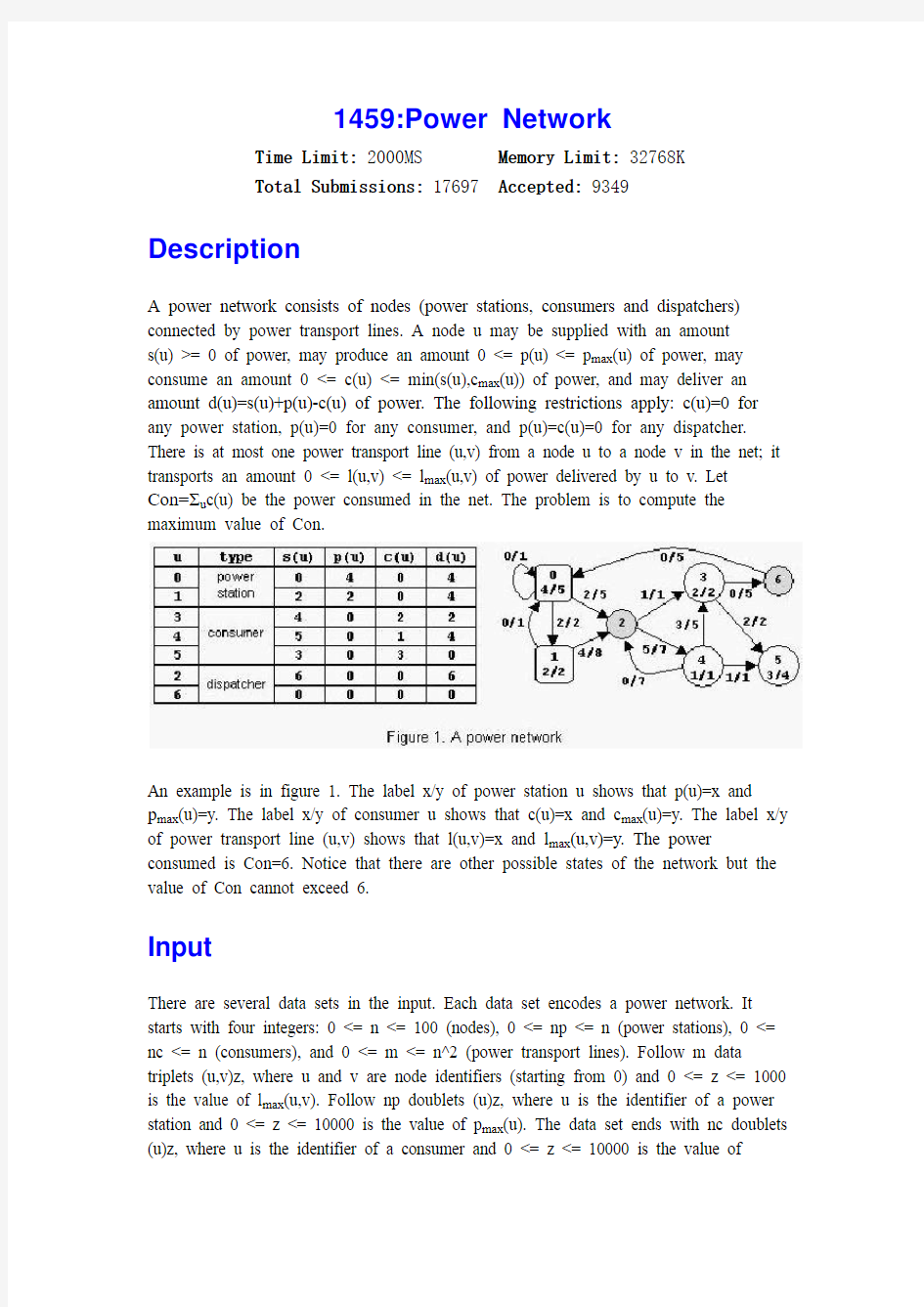
s(u) >= 0 of power, may produce an amount 0 <= p(u) <= p max(u) of power, may consume an amount 0 <= c(u) <= min(s(u),c max(u)) of power, and may deliver an amount d(u)=s(u)+p(u)-c(u) of power. The following restrictions apply: c(u)=0 for any power station, p(u)=0 for any consumer, and p(u)=c(u)=0 for any dispatcher. There is at most one power transport line (u,v) from a node u to a node v in the net; it transports an amount 0 <= l(u,v) <= l max(u,v) of power delivered by u to v. Let

Con=Σu c(u) be the power consumed in the net. The problem is to compute the maximum value of Con.

An example is in figure 1. The label x/y of power station u shows that p(u)=x and

p max(u)=y. The label x/y of consumer u shows that c(u)=x and c max(u)=y. The label x/y of power transport line (u,v) shows that l(u,v)=x and l max(u,v)=y. The power consumed is Con=6. Notice that there are other possible states of the network but the value of Con cannot exceed 6.

Input

There are several data sets in the input. Each data set encodes a power network. It starts with four integers: 0 <= n <= 100 (nodes), 0 <= np <= n (power stations), 0 <= nc <= n (consumers), and 0 <= m <= n^2 (power transport lines). Follow m data triplets (u,v)z, where u and v are node identifiers (starting from 0) and 0 <= z <= 1000 is the value of l max(u,v). Follow np doublets (u)z, where u is the identifier of a power station and 0 <= z <= 10000 is the value of p max(u). The data set ends with nc doublets (u)z, where u is the identifier of a consumer and 0 <= z <= 10000 is the value of

c max(u). All input numbers are integers. Except the (u,v)z triplets an

d th

e (u)z doublets, which do not contain white spaces, white spaces can occur freely in input. Input data terminate with an end o

f file and are correct.

Output

For each data set from the input, the program prints on the standard output the maximum amount of power that can be consumed in the corresponding network. Each result has an integral value and is printed from the beginning of a separate line. Sample Input

2 1 1 2 (0,1)20 (1,0)10 (0)15 (1)20

7 2 3 13 (0,0)1 (0,1)2 (0,2)5 (1,0)1 (1,2)8 (2,3)1 (2,4)7 (3,5)2 (3,6)5 (4,2)7 (4,3)5 (4,5)1 (6,0)5

(0)5 (1)2 (3)2 (4)1 (5)4

Sample Output

15

6

Hint

The sample input contains two data sets. The first data set encodes a network with 2 nodes, power station 0 with pmax(0)=15 and consumer 1 with cmax(1)=20, and 2 power transport lines with lmax(0,1)=20 and lmax(1,0)=10. The maximum value of Con is 15. The second data set encodes the network from figure 1.

Source

Southeastern Europe 2003

2426:ACM Computer Factory

Time Limit: 1000MS Memory Limit: 65536K

Total Submissions: 3986 Accepted: 1325 Special Judge Description

As you know, all the computers used for ACM contests must be identical, so the participants compete on equal terms. That is why all these computers are historically produced at the same factory.

Every ACM computer consists of P parts. When all these parts are present, the computer is ready and can be shipped to one of the numerous ACM contests.

Computer manufacturing is fully automated by using N various machines. Each machine removes some parts from a half-finished computer and adds some new parts (removing of parts is sometimes necessary as the parts cannot be added to a computer in arbitrary order). Each machine is described by its performance (measured in computers per hour), input and output specification.

Input specification describes which parts must be present in a half-finished computer for the machine to be able to operate on it. The specification is a set of P numbers 0, 1 or 2 (one number for each part), where 0 means that corresponding part must not be present, 1 — the part is required, 2 — presence of the part doesn't matter.

Output specification describes the result of the operation, and is a set of P numbers 0 or 1, where 0 means that the part is absent, 1 — the part is present.

The machines are connected by very fast production lines so that delivery time is negligibly small compared to production time.

After many years of operation the overall performance of the ACM Computer Factory became insufficient for satisfying the growing contest needs. That is why ACM directorate decided to upgrade the factory.

As different machines were installed in different time periods, they were often not optimally connected to the existing factory machines. It was noted that the easiest way to upgrade the factory is to rearrange production lines. ACM directorate decided to entrust you with solving this problem.

Input

Input file contains integers P N, then N descriptions of the machines. The description of i th machine is represented as by 2 P + 1 integers Q i S i,1Si,2...S i,P D i,1D i,2...D i,P, where Q i specifies performance, S i,j— input specification for part j, D i,k— output specification for part k.

Constraints

1 ≤ P≤ 10, 1 ≤ N ≤ 50, 1 ≤ Q i≤ 10000

Output

Output the maximum possible overall performance, then M— number of connections that must be made, then M descriptions of the connections. Each connection between machines A and B must be described by three positive numbers A B W, where W is the number of computers delivered from A to B per hour.

If several solutions exist, output any of them.

Sample Input

Sample input 1

3 4

15 0 0 0 0 1 0

10 0 0 0 0 1 1

30 0 1 2 1 1 1

3 0 2 1 1 1 1

Sample input 2

3 5

5 0 0 0 0 1 0

100 0 1 0 1 0 1

3 0 1 0 1 1 0

1 1 0 1 1 1 0

300 1 1 2 1 1 1

Sample input 3

2 2

100 0 0 1 0

200 0 1 1 1

Sample Output

Sample output 1

25 2

1 3 15

2 3 10

Sample output 2

4 5

1 3 3

3 5 3

1 2 1

2 4 1

4 5 1

Sample output 3

0 0

Hint

Bold texts appearing in the sample sections are informative and do not form part of the actual data.

Source

Northeastern Europe 2005, Far-Eastern Subregion