Rapid Object Detection using a Boosted cascade of simple features

A CCEPTED C ONFERENCE ON C OMPUTER V ISION AND P ATTERN R ECOGNITION2001 Rapid Object Detection using a Boosted Cascade of Simple

Features

Paul Viola Michael Jones viola@https://www.360docs.net/doc/7110167247.html, mjones@https://www.360docs.net/doc/7110167247.html, Mitsubishi Electric Research Labs Compaq CRL 201Broadway,8th FL One Cambridge Center

Cambridge,MA02139Cambridge,MA02142

Abstract

This paper describes a machine learning approach for vi-sual object detection which is capable of processing images extremely rapidly and achieving high detection rates.This work is distinguished by three key contributions.The?rst is the introduction of a new image representation called the “Integral Image”which allows the features used by our de-tector to be computed very quickly.The second is a learning algorithm,based on AdaBoost,which selects a small num-ber of critical visual features from a larger set and yields extremely ef?cient classi?ers[6].The third contribution is a method for combining increasingly more complex classi-?ers in a“cascade”which allows background regions of the image to be quickly discarded while spending more compu-tation on promising object-like regions.The cascade can be viewed as an object speci?c focus-of-attention mechanism which unlike previous approaches provides statistical guar-antees that discarded regions are unlikely to contain the ob-ject of interest.In the domain of face detection the system yields detection rates comparable to the best previous https://www.360docs.net/doc/7110167247.html,ed in real-time applications,the detector runs at 15frames per second without resorting to image differenc-ing or skin color detection.

1.Introduction

This paper brings together new algorithms and insights to construct a framework for robust and extremely rapid object detection.This framework is demonstrated on,and in part motivated by,the task of face detection.Toward this end we have constructed a frontal face detection system which achieves detection and false positive rates which are equiv-alent to the best published results[16,12,15,11,1].This face detection system is most clearly distinguished from previous approaches in its ability to detect faces extremely rapidly.Operating on384by288pixel images,faces are de-

tected at15frames per second on a conventional700MHz Intel Pentium III.In other face detection systems,auxiliary information,such as image differences in video sequences, or pixel color in color images,have been used to achieve high frame rates.Our system achieves high frame rates working only with the information present in a single grey scale image.These alternative sources of information can also be integrated with our system to achieve even higher frame rates.

There are three main contributions of our object detec-tion framework.We will introduce each of these ideas brie?y below and then describe them in detail in subsequent sections.

The?rst contribution of this paper is a new image repre-sentation called an integral image that allows for very fast feature evaluation.Motivated in part by the work of Papa-georgiou et al.our detection system does not work directly with image intensities[10].Like these authors we use a set of features which are reminiscent of Haar Basis func-tions(though we will also use related?lters which are more complex than Haar?lters).In order to compute these fea-tures very rapidly at many scales we introduce the integral image representation for images.The integral image can be computed from an image using a few operations per pixel.

Once computed,any one of these Harr-like features can be computed at any scale or location in constant time.

The second contribution of this paper is a method for constructing a classi?er by selecting a small number of im-portant features using AdaBoost[6].Within any image sub-window the total number of Harr-like features is very large, far larger than the number of pixels.In order to ensure fast classi?cation,the learning process must exclude a large ma-jority of the available features,and focus on a small set of critical features.Motivated by the work of Tieu and Viola, feature selection is achieved through a simple modi?cation of the AdaBoost procedure:the weak learner is constrained so that each weak classi?er returned can depend on only a 1

single feature[2].As a result each stage of the boosting process,which selects a new weak classi?er,can be viewed as a feature selection process.AdaBoost provides an effec-tive learning algorithm and strong bounds on generalization performance[13,9,10].

The third major contribution of this paper is a method for combining successively more complex classi?ers in a cascade structure which dramatically increases the speed of the detector by focusing attention on promising regions of the image.The notion behind focus of attention approaches is that it is often possible to rapidly determine where in an image an object might occur[17,8,1].More complex pro-cessing is reserved only for these promising regions.The key measure of such an approach is the“false negative”rate of the attentional process.It must be the case that all,or almost all,object instances are selected by the attentional ?lter.

We will describe a process for training an extremely sim-ple and ef?cient classi?er which can be used as a“super-vised”focus of attention operator.The term supervised refers to the fact that the attentional operator is trained to detect examples of a particular class.In the domain of face detection it is possible to achieve fewer than1%false neg-atives and40%false positives using a classi?er constructed from two Harr-like features.The effect of this?lter is to reduce by over one half the number of locations where the ?nal detector must be evaluated.

Those sub-windows which are not rejected by the initial classi?er are processed by a sequence of classi?ers,each slightly more complex than the last.If any classi?er rejects the sub-window,no further processing is performed.The structure of the cascaded detection process is essentially that of a degenerate decision tree,and as such is related to the work of Geman and colleagues[1,4].

An extremely fast face detector will have broad prac-tical applications.These include user interfaces,image databases,and teleconferencing.In applications where rapid frame-rates are not necessary,our system will allow for signi?cant additional post-processing and analysis.In addition our system can be implemented on a wide range of small low power devices,including hand-helds and embed-ded processors.In our lab we have implemented this face detector on the Compaq iPaq handheld and have achieved detection at two frames per second(this device has a low power200mips Strong Arm processor which lacks?oating point hardware).

The remainder of the paper describes our contributions and a number of experimental results,including a detailed description of our experimental methodology.Discussion of closely related work takes place at the end of each sec-tion.

2.Features

Our object detection procedure classi?es images based on the value of simple features.There are many motivations

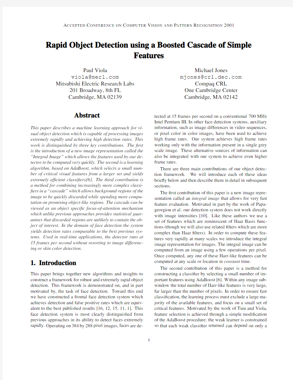
Figure1:Example rectangle features shown relative to the enclosing detection window.The sum of the pixels which lie within the white rectangles are subtracted from the sum of pixels in the grey rectangles.Two-rectangle features are shown in(A)and(B).Figure(C)shows a three-rectangle feature,and(D)a four-rectangle feature.

for using features rather than the pixels directly.The most common reason is that features can act to encode ad-hoc domain knowledge that is dif?cult to learn using a?nite quantity of training data.For this system there is also a second critical motivation for features:the feature based system operates much faster than a pixel-based system.

The simple features used are reminiscent of Haar basis functions which have been used by Papageorgiou et al.[10]. More speci?cally,we use three kinds of features.The value of a two-rectangle feature is the difference between the sum of the pixels within two rectangular regions.The regions have the same size and shape and are horizontally or ver-tically adjacent(see Figure1).A three-rectangle feature computes the sum within two outside rectangles subtracted from the sum in a center rectangle.Finally a four-rectangle feature computes the difference between diagonal pairs of rectangles.

Given that the base resolution of the detector is24x24, the exhaustive set of rectangle features is quite large,over 180,000.Note that unlike the Haar basis,the set of rectan-gle features is overcomplete1.

2.1.Integral Image

Rectangle features can be computed very rapidly using an intermediate representation for the image which we call the integral image.2The integral image at location contains the sum of the pixels above and to the left of,inclusive:

Figure2:The sum of the pixels within rectangle can be computed with four array references.The value of the inte-gral image at location1is the sum of the pixels in rectangle .The value at location2is,at location3is, and at location4is.The sum within can be computed as.

where is the integral image and is the origi-nal https://www.360docs.net/doc/7110167247.html,ing the following pair of recurrences:

(1)

(2) (where is the cumulative row sum,, and)the integral image can be computed in one pass over the original image.

Using the integral image any rectangular sum can be computed in four array references(see Figure2).Clearly the difference between two rectangular sums can be com-puted in eight references.Since the two-rectangle features de?ned above involve adjacent rectangular sums they can be computed in six array references,eight in the case of the three-rectangle features,and nine for four-rectangle fea-tures.

2.2.Feature Discussion

Rectangle features are somewhat primitive when compared with alternatives such as steerable?lters[5,7].Steerable?l-ters,and their relatives,are excellent for the detailed analy-sis of boundaries,image compression,and texture analysis. In contrast rectangle features,while sensitive to the pres-ence of edges,bars,and other simple image structure,are quite coarse.Unlike steerable?lters the only orientations available are vertical,horizontal,and diagonal.The set of rectangle features do however provide a rich image repre-sentation which supports effective learning.In conjunction with the integral image,the ef?ciency of the rectangle fea-ture set provides ample compensation for their limited?ex-ibility.

3.Learning Classi?cation Functions Given a feature set and a training set of positive and neg-ative images,any number of machine learning approaches

could be used to learn a classi?cation function.In our sys-tem a variant of AdaBoost is used both to select a small set of features and train the classi?er[6].In its original form, the AdaBoost learning algorithm is used to boost the clas-si?cation performance of a simple(sometimes called weak) learning algorithm.There are a number of formal guaran-tees provided by the AdaBoost learning procedure.Freund and Schapire proved that the training error of the strong classi?er approaches zero exponentially in the number of rounds.More importantly a number of results were later proved about generalization performance[14].The key insight is that generalization performance is related to the margin of the examples,and that AdaBoost achieves large margins rapidly.

Recall that there are over180,000rectangle features as-sociated with each image sub-window,a number far larger than the number of pixels.Even though each feature can be computed very ef?ciently,computing the complete set is prohibitively expensive.Our hypothesis,which is borne out by experiment,is that a very small number of these features can be combined to form an effective classi?er.The main challenge is to?nd these features.

In support of this goal,the weak learning algorithm is designed to select the single rectangle feature which best separates the positive and negative examples(this is similar to the approach of[2]in the domain of image database re-trieval).For each feature,the weak learner determines the optimal threshold classi?cation function,such that the min-imum number of examples are misclassi?ed.A weak clas-si?er thus consists of a feature,a threshold and

a parity indicating the direction of the inequality sign:

if

otherwise

Here is a24x24pixel sub-window of an image.See Ta-ble1for a summary of the boosting process.

In practice no single feature can perform the classi?ca-tion task with low error.Features which are selected in early rounds of the boosting process had error rates between0.1 and0.3.Features selected in later rounds,as the task be-comes more dif?cult,yield error rates between0.4and0.5.

3.1.Learning Discussion

Many general feature selection procedures have been pro-posed(see chapter8of[18]for a review).Our?nal appli-cation demanded a very aggressive approach which would discard the vast majority of features.For a similar recogni-tion problem Papageorgiou et al.proposed a scheme for fea-ture selection based on feature variance[10].They demon-strated good results selecting37features out of a total1734 features.

Roth et al.propose a feature selection process based on the Winnow exponential perceptron learning rule[11].

The Winnow learning process converges to a solution where many of these weights are zero.Nevertheless a very large

3

Given example images where

for negative and positive examples respec-tively.

Initialize weights for respec-

tively,where and are the number of negatives and

positives respectively.

For:

1.Normalize the weights,

.

The?nal strong classi?er is:

Table1:The AdaBoost algorithm for classi?er learn-ing.Each round of boosting selects one feature from the 180,000potential features.

number of features are retained(perhaps a few hundred or thousand).

3.2.Learning Results

While details on the training and performance of the?nal system are presented in Section5,several simple results merit discussion.Initial experiments demonstrated that a frontal face classi?er constructed from200features yields a detection rate of95%with a false positive rate of1in 14084.These results are compelling,but not suf?cient for many real-world tasks.In terms of computation,this clas-si?er is probably faster than any other published system, requiring0.7seconds to scan an384by288pixel image. Unfortunately,the most straightforward technique for im-proving detection performance,adding features to the clas-si?er,directly increases computation time.

For the task of face detection,the initial rectangle fea-tures selected by AdaBoost are meaningful and easily inter-preted.The?rst feature selected seems to focus on the prop-erty that the region of the eyes is often darker than the

region

Figure3:The?rst and second features selected by Ad-aBoost.The two features are shown in the top row and then overlayed on a typical training face in the bottom row.The ?rst feature measures the difference in intensity between the region of the eyes and a region across the upper cheeks.The feature capitalizes on the observation that the eye region is often darker than the cheeks.The second feature compares the intensities in the eye regions to the intensity across the bridge of the nose.

of the nose and cheeks(see Figure3).This feature is rel-atively large in comparison with the detection sub-window, and should be somewhat insensitive to size and location of the face.The second feature selected relies on the property that the eyes are darker than the bridge of the nose.

4.The Attentional Cascade

This section describes an algorithm for constructing a cas-cade of classi?ers which achieves increased detection per-formance while radically reducing computation time.The key insight is that smaller,and therefore more ef?cient, boosted classi?ers can be constructed which reject many of the negative sub-windows while detecting almost all posi-tive instances(i.e.the threshold of a boosted classi?er can be adjusted so that the false negative rate is close to zero).

Simpler classi?ers are used to reject the majority of sub-windows before more complex classi?ers are called upon to achieve low false positive rates.

The overall form of the detection process is that of a de-generate decision tree,what we call a“cascade”(see Fig-ure4).A positive result from the?rst classi?er triggers the evaluation of a second classi?er which has also been ad-justed to achieve very high detection rates.A positive result from the second classi?er triggers a third classi?er,and so on.A negative outcome at any point leads to the immediate rejection of the sub-window.

Stages in the cascade are constructed by training clas-si?ers using AdaBoost and then adjusting the threshold to minimize false negatives.Note that the default AdaBoost threshold is designed to yield a low error rate on the train-ing data.In general a lower threshold yields higher detec-4

Reject Sub?window

Figure4:Schematic depiction of a the detection cascade.

A series of classi?ers are applied to every sub-window.The initial classi?er eliminates a large number of negative exam-ples with very little processing.Subsequent layers eliminate additional negatives but require additional computation.Af-ter several stages of processing the number of sub-windows have been reduced radically.Further processing can take any form such as additional stages of the cascade(as in our detection system)or an alternative detection system.

tion rates and higher false positive rates.

For example an excellent?rst stage classi?er can be con-structed from a two-feature strong classi?er by reducing the threshold to minimize false negatives.Measured against a validation training set,the threshold can be adjusted to de-tect100%of the faces with a false positive rate of40%.See Figure3for a description of the two features used in this classi?er.

Computation of the two feature classi?er amounts to about60microprocessor instructions.It seems hard to imagine that any simpler?lter could achieve higher rejec-tion rates.By comparison,scanning a simple image tem-plate,or a single layer perceptron,would require at least20 times as many operations per sub-window.

The structure of the cascade re?ects the fact that within any single image an overwhelming majority of sub-windows are negative.As such,the cascade attempts to re-ject as many negatives as possible at the earliest stage pos-sible.While a positive instance will trigger the evaluation of every classi?er in the cascade,this is an exceedingly rare event.

Much like a decision tree,subsequent classi?ers are trained using those examples which pass through all the previous stages.As a result,the second classi?er faces a more dif?cult task than the?rst.The examples which make it through the?rst stage are“harder”than typical exam-ples.The more dif?cult examples faced by deeper classi-?ers push the entire receiver operating characteristic(ROC) curve downward.At a given detection rate,deeper classi-?ers have correspondingly higher false positive rates.4.1.Training a Cascade of Classi?ers

The cascade training process involves two types of trade-offs.In most cases classi?ers with more features will achieve higher detection rates and lower false positive rates. At the same time classi?ers with more features require more time to compute.In principle one could de?ne an optimiza-tion framework in which:i)the number of classi?er stages, ii)the number of features in each stage,and iii)the thresh-old of each stage,are traded off in order to minimize the expected number of evaluated features.Unfortunately?nd-ing this optimum is a tremendously dif?cult problem.

In practice a very simple framework is used to produce an effective classi?er which is highly ef?cient.Each stage in the cascade reduces the false positive rate and decreases the detection rate.A target is selected for the minimum reduction in false positives and the maximum decrease in detection.Each stage is trained by adding features until the target detection and false positives rates are met(these rates are determined by testing the detector on a validation set). Stages are added until the overall target for false positive and detection rate is met.

4.2.Detector Cascade Discussion

The complete face detection cascade has38stages with over 6000features.Nevertheless the cascade structure results in fast average detection times.On a dif?cult dataset,con-taining507faces and75million sub-windows,faces are detected using an average of10feature evaluations per sub-window.In comparison,this system is about15times faster than an implementation of the detection system constructed by Rowley et al.3[12]

A notion similar to the cascade appears in the face de-tection system described by Rowley et al.in which two de-tection networks are used[12].Rowley et https://www.360docs.net/doc/7110167247.html,ed a faster yet less accurate network to prescreen the image in order to ?nd candidate regions for a slower more accurate network. Though it is dif?cult to determine exactly,it appears that Rowley et al.’s two network face system is the fastest exist-ing face detector.4

The structure of the cascaded detection process is es-sentially that of a degenerate decision tree,and as such is related to the work of Amit and Geman[1].Unlike tech-niques which use a?xed detector,Amit and Geman propose an alternative point of view where unusual co-occurrences of simple image features are used to trigger the evaluation of a more complex detection process.In this way the full detection process need not be evaluated at many of the po-tential image locations and scales.While this basic insight

is very valuable,in their implementation it is necessary to ?rst evaluate some feature detector at every location.These features are then grouped to?nd unusual co-occurrences.In practice,since the form of our detector and the features that it uses are extremely ef?cient,the amortized cost of evalu-ating our detector at every scale and location is much faster than?nding and grouping edges throughout the image.

In recent work Fleuret and Geman have presented a face detection technique which relies on a“chain”of tests in or-der to signify the presence of a face at a particular scale and location[4].The image properties measured by Fleuret and Geman,disjunctions of?ne scale edges,are quite different than rectangle features which are simple,exist at all scales, and are somewhat interpretable.The two approaches also differ radically in their learning philosophy.The motivation for Fleuret and Geman’s learning process is density estima-tion and density discrimination,while our detector is purely discriminative.Finally the false positive rate of Fleuret and Geman’s approach appears to be higher than that of previ-ous approaches like Rowley et al.and this approach.Un-fortunately the paper does not report quantitative results of this kind.The included example images each have between 2and10false positives.

5Results

A38layer cascaded classi?er was trained to detect frontal upright faces.To train the detector,a set of face and non-face training images were used.The face training set con-sisted of4916hand labeled faces scaled and aligned to a base resolution of24by24pixels.The faces were ex-tracted from images downloaded during a random crawl of the world wide web.Some typical face examples are shown in Figure5.The non-face subwindows used to train the detector come from9544images which were manually in-spected and found to not contain any faces.There are about 350million subwindows within these non-face images.

The number of features in the?rst?ve layers of the de-tector is1,10,25,25and50features respectively.The remaining layers have increasingly more features.The total number of features in all layers is6061.

Each classi?er in the cascade was trained with the4916 training faces(plus their vertical mirror images for a total of9832training faces)and10,000non-face sub-windows (also of size24by24pixels)using the Adaboost training procedure.For the initial one feature classi?er,the non-face training examples were collected by selecting random sub-windows from a set of9544images which did not con-tain faces.The non-face examples used to train subsequent layers were obtained by scanning the partial cascade across the non-face images and collecting false positives.A max-imum of10000such non-face sub-windows were collected for each layer.

Speed of the Final

Detector Figure5:Example of frontal upright face images used for training.

The speed of the cascaded detector is directly related to the number of features evaluated per scanned sub-window. Evaluated on the MIT+CMU test set[12],an average of10 features out of a total of6061are evaluated per sub-window. This is possible because a large majority of sub-windows are rejected by the?rst or second layer in the cascade.On a700Mhz Pentium III processor,the face detector can pro-cess a384by288pixel image in about.067seconds(us-ing a starting scale of1.25and a step size of1.5described below).This is roughly15times faster than the Rowley-Baluja-Kanade detector[12]and about600times faster than the Schneiderman-Kanade detector[15].

Image Processing

All example sub-windows used for training were vari-ance normalized to minimize the effect of different light-ing conditions.Normalization is therefore necessary during detection as well.The variance of an image sub-window can be computed quickly using a pair of integral images. Recall that

Detector False detections

316595

76.1%91.4%92.1%93.9%

81.1%92.1%93.1%93.7%

83.2%--90.1%

----

--(94.8%)-

Table2:Detection rates for various numbers of false positives on the MIT+CMU test set containing130images and507 faces.

scale with the same cost.Good results were obtained using a set of scales a factor of1.25apart.

The detector is also scanned across location.Subsequent locations are obtained by shifting the window some number of pixels.This shifting process is affected by the scale of the detector:if the current scale is the window is shifted by,where is the rounding operation.

The choice of affects both the speed of the detector as well as accuracy.The results we present are for. We can achieve a signi?cant speedup by setting

with only a slight decrease in accuracy.

Integration of Multiple Detections

Since the?nal detector is insensitive to small changes in translation and scale,multiple detections will usually occur around each face in a scanned image.The same is often true of some types of false positives.In practice it often makes sense to return one?nal detection per face.Toward this end it is useful to postprocess the detected sub-windows in order to combine overlapping detections into a single detection.

In these experiments detections are combined in a very simple fashion.The set of detections are?rst partitioned into disjoint subsets.Two detections are in the same subset if their bounding regions overlap.Each partition yields a single?nal detection.The corners of the?nal bounding region are the average of the corners of all detections in the set.

Experiments on a Real-World Test Set

We tested our system on the MIT+CMU frontal face test set[12].This set consists of130images with507labeled frontal faces.A ROC curve showing the performance of our detector on this test set is shown in Figure6.To create the ROC curve the threshold of the?nal layer classi?er is ad-justed from to.Adjusting the threshold to

will yield a detection rate of0.0and a false positive rate of0.0.Adjusting the threshold to,however,increases both the detection rate and false positive rate,but only to a certain point.Neither rate can be higher than the rate of the detection cascade minus the?nal layer.In effect,a thresh-old of is equivalent to removing that layer.Further increasing the detection and false positive rates requires de-creasing the threshold of the next classi?er in the cascade.

Thus,in order to construct a complete ROC curve,classi?er layers are removed.We use the number of false positives as opposed to the rate of false positives for the x-axis of the ROC curve to facilitate comparison with other systems.To compute the false positive rate,simply divide by the total number of sub-windows scanned.In our experiments,the number of sub-windows scanned is75,081,800.

Unfortunately,most previous published results on face detection have only included a single operating regime(i.e.

single point on the ROC curve).To make comparison with our detector easier we have listed our detection rate for the false positive rates reported by the other systems.Table2 lists the detection rate for various numbers of false detec-tions for our system as well as other published systems.For the Rowley-Baluja-Kanade results[12],a number of differ-ent versions of their detector were tested yielding a number of different results they are all listed in under the same head-ing.For the Roth-Yang-Ahuja detector[11],they reported their result on the MIT+CMU test set minus5images con-taining line drawn faces removed.

Figure7shows the output of our face detector on some test images from the MIT+CMU test set.

A simple voting scheme to further improve results

In table2we also show results from running three de-tectors(the38layer one described above plus two similarly trained detectors)and outputting the majority vote of the three detectors.This improves the detection rate as well as eliminating more false positives.The improvement would be greater if the detectors were more independent.The cor-relation of their errors results in a modest improvement over the best single detector.

6Conclusions

We have presented an approach for object detection which minimizes computation time while achieving high detection accuracy.The approach was used to construct a face de-tection system which is approximately15faster than any previous approach.

This paper brings together new algorithms,representa-tions,and insights which are quite generic and may well 7

Figure 7:Output of our face detector on a number of test images from the MIT+CMU test

set.

Figure 6:ROC curve for our face detector on the MIT+CMU test set.The detector was run using a step size of 1.0and starting scale of 1.0(75,081,800sub-windows scanned).

have broader application in computer vision and image pro-cessing.

Finally this paper presents a set of detailed experiments on a dif?cult face detection dataset which has been widely studied.This dataset includes faces under a very wide range of conditions including:illumination,scale,pose,and cam-era variation.Experiments on such a large and complex dataset are dif?cult and time consuming.Nevertheless sys-tems which work under these conditions are unlikely to be brittle or limited to a single set of conditions.More impor-tantly conclusions drawn from this dataset are unlikely to be experimental artifacts.

References

[1]Y .Amit,D.Geman,and K.Wilder.Joint induction of shape

features and tree classi?ers,1997.[2]Anonymous.Anonymous.In Anonymous ,2000.

[3] F.Crow.Summed-area tables for texture mapping.In

Proceedings of SIGGRAPH ,volume 18(3),pages 207–212,1984.[4] F.Fleuret and D.Geman.Coarse-to-?ne face detection.Int.

https://www.360docs.net/doc/7110167247.html,puter Vision ,2001.[5]William T.Freeman and Edward H.Adelson.The design

and use of steerable ?lters.IEEE Transactions on Pattern Analysis and Machine Intelligence ,13(9):891–906,1991.[6]Yoav Freund and Robert E.Schapire.A decision-theoretic

generalization of on-line learning and an application to boosting.In Computational Learning Theory:Eurocolt ’95,pages 23–37.Springer-Verlag,1995.[7]H.Greenspan,S.Belongie,R.Gooodman,P.Perona,S.Rak-shit,and C.Anderson.Overcomplete steerable pyramid ?l-ters and rotation invariance.In Proceedings of the IEEE Con-ference on Computer Vision and Pattern Recognition ,1994.

[8]L.Itti,C.Koch,and E.Niebur.A model of saliency-based

visual attention for rapid scene analysis.IEEE Patt.Anal.Mach.Intell.,20(11):1254–1259,November 1998.[9]Edgar Osuna,Robert Freund,and Federico Girosi.Training

support vector machines:an application to face detection.In Proceedings of the IEEE Conference on Computer Vision and Pattern Recognition ,1997.[10] C.Papageorgiou,M.Oren,and T.Poggio.A general frame-work for object detection.In International Conference on Computer Vision ,1998.[11] D.Roth,M.Yang,and N.Ahuja.A snowbased face detector.

In Neural Information Processing 12,2000.[12]H.Rowley,S.Baluja,and T.Kanade.Neural network-based

face detection.In IEEE Patt.Anal.Mach.Intell.,volume 20,pages 22–38,1998.[13]R.E.Schapire,Y .Freund,P.Bartlett,and W.S.Lee.Boost-ing the margin:a new explanation for the effectiveness of voting methods.Ann.Stat.,26(5):1651–1686,1998.[14]Robert E.Schapire,Yoav Freund,Peter Bartlett,and

Wee Sun Lee.Boosting the margin:A new explanation for the effectiveness of voting methods.In Proceedings of the Fourteenth International Conference on Machine Learning ,1997.[15]H.Schneiderman and T.Kanade.A statistical method for 3D

object detection applied to faces and cars.In International Conference on Computer Vision ,2000.

8

[16]K.Sung and T.Poggio.Example-based learning for view-

based face detection.In IEEE Patt.Anal.Mach.Intell.,vol-

ume20,pages39–51,1998.

[17]J.K.Tsotsos,S.M.Culhane,W.Y.K.Wai,https://www.360docs.net/doc/7110167247.html,i,N.Davis,

and F.Nu?o.Modeling visual-attention via selective tun-

ing.Arti?cial Intelligence Journal,78(1-2):507–545,Octo-

ber1995.

[18]Andrew Webb.Statistical Pattern Recognition.Oxford Uni-

versity Press,New York,1999.

9