数字信号处理答案10

Chapter 10 Solutions

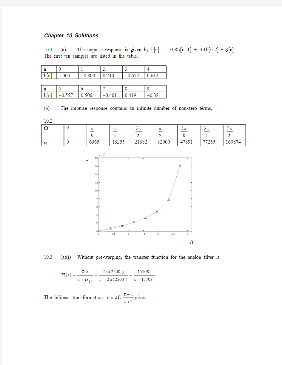
10.1 (a) The impulse response is given by h[n] = –0.8h[n –1] + 0.1h[n –2] + δ[n]. The first ten samples are listed in the table.

(b) The impulse response contains an infinite number of non-zero terms.

10.3 (a)(i) Without pre-warping, the transfer function for the analog filter is

15708

s 15708)

2500(2s )2500(2s )s (H 1

p 1p +=

π+π=

ω+ω=

The bilinear transformation 1

z 1z f 2s S +-=gives

00921.01)

1(4954.015708

z 1z 16000

15708)z (H ---+=

++-=

(ii)

The analog frequency 2.5 kHz is converted to a digital frequency Ωp1 =

8000/)2500(2π =1.9635 rads. This frequency is pre-warped to the analog frequency

tan

f 21p S 1p Ω=ω= 23946 rad/sec, which makes the transfer function for the analo

g filter

23946

s 23946s )s (H 1

p 1p +=

ω+ω=

After the bilinear transformation, the digital transfer function is obtained:

1989.01)

1(6.023946

z 1z 16000

23946)z (H --++=

++-=

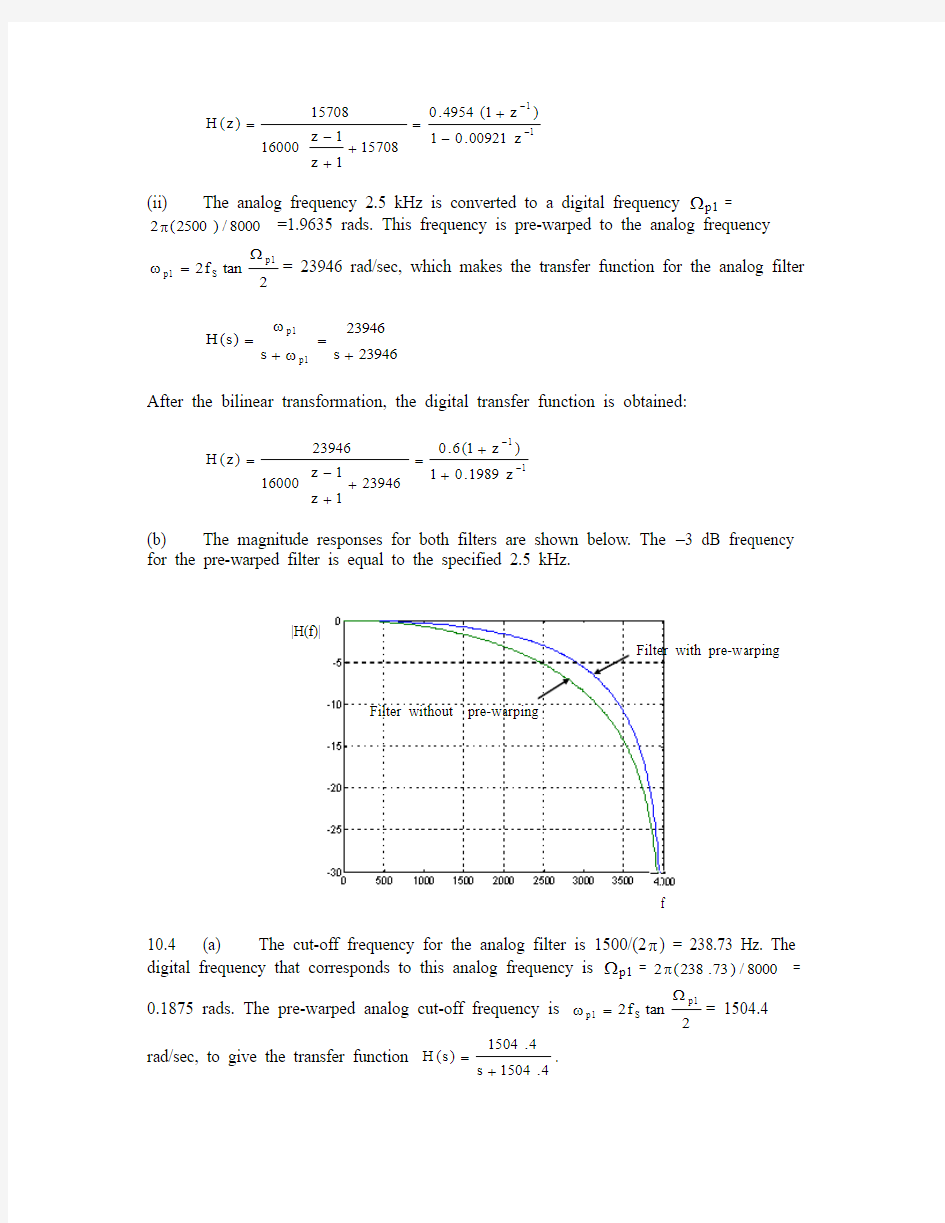
(b) The magnitude responses for both filters are shown below. The –3 dB frequency for the pre-warped filter is equal to the specified 2.5 kHz.

10.4 (a) The cut-off frequency for the analog filter is 1500/(2π) = 238.73 Hz. The digital frequency that corresponds to this analog frequency is Ωp1 = 8000/)73.238(2π = 0.1875 rads. The pre-warped analog cut-off frequency is 2

tan f 21p S 1p Ω=ω= 1504.4

rad/sec, to give the transfer function 4

.1504s 4.1504)s (H +=

Filter with pre-warping |H(f)| f

(b) Use the bilinear transformation to get the digital transfer function

8281.01)

z 1(0859.04

.15041

z 1z 16000

4.1504)z (H ---+=

++-=

The frequency response is Ω

-Ω--+=

Ωj j e

8281.01)

e 1(0859.0)(H . The magnitude response

may be found by taking the magnitudes of this expression for several values of Ω. It is plotted below against frequency in Hz.

(e) The magnitude for the analog transfer function is

.15044.1504)(H +ω=

The shape of the digital filter may be found by substituting 2

tan f 2S Ω=ω:

S 4

.15042tan 160004

.15044

.15042tan f 24

.1504)(H +??? ?

?Ω=

+??? ?

?Ω=

This function may be plotted for various values of Ω. The magnitude response is plotted below against digital frequency in rads. When digital frequencies are converted to frequencies in Hz, the plot becomes identical to the one in part (d).

10.5 The –3 dB frequency for this filter is 1 kHz. This is the edge of the pass band. The stop band edge can chosen at any convenient place. For example, the gain at 3 kHz is about –46 dB. The stop band ripple is given by 20log δs = –46, or δs = 0.005. The digital frequencies at the edges of the pass band and stop band are

Ωp1 = π

=π

25.08000

10002f f 2S

1p radians

Ωs1 =π=π

=π

75.08000

30002f f 2S

1s radians

ωp1 = 4.66272

tan

f 21p S =Ω rad/sec

ωs1 = 4.386272

tan

f 21s S =Ω rad/sec

The order for the filter is

10.6 The stop band attenuation gives 20log δs = –28, or δs = 0.0398. Ωp1 = π=π

=π

542.024000

65002f f 2S

1p radians

4.66274.38627log 21)00

5.0(1

log log 211log n 21

p 1s 2s =??

? ?????? ??-=??

? ?

?ωω???? ??-δ≥|H(

Ωs1 =π=π

=π

667.024000

80002f f 2S

1s radians

ωp1 = 4.547912

tan

f 21p S =Ω rad/sec

ωs1 = 1.832392

tan

f 21s S =Ω rad/sec

The order for the filter can be calculated using

so an order of 8 should be chosen. For this order, the magnitude response for the analog filter is given by

4.547911

1)(H 16

p +??

? ??ω=+???

? ??ωω=

Therefore, the transfer function for the digital filter is

4.547912tan 480001

4.547912tan f 21

)(H 16

+?????

Ω=

+?????

Ω=

The plot of |H(Ω)| versus Ω is the same as the plot of |H(f)| versus f, except that, along the horizontal axis, digital frequencies between 0 and π radians are converted to

frequencies between 0 and 12000 Hz (half the sampling rate). The magnitude response is shown below. The eighth order filter matches the specifications.

.74.547911.83239log 21

)0398.0(1

log log 211log n 21

p 1

s 2s =??? ?????? ??-=???

? ??ωω???? ??-δ≥

10.7 The stop band attenuation gives 20log δs = –35, or δs = 0.01778.

Ωp1 = π

=π

625.08000

25002f f 2S

1p radians

Ωs1 =π=π

=π

95.08000

38002f f 2S

1s radians

ωp1 = 239462

tan

f 21p S =Ω rad/sec

ωs1 = 2032992

tan

f 21s S =Ω rad/sec

The order for the filter can be calculated using

so an order of 2 should be chosen.

10.8 The 600 Hz transition width puts the stop band edge at 1.9 kHz. The digital pass band edge frequencies are

Ωp1 = π=π

=π

26.010000

13002f f 2S

1p radians

|H(f)|

.123946203299

log 21)01778.0(1log log 211log n 2

p 1

s 2s =??

? ?????? ??-=??

? ??ωω??

?? ??-δ≥

Ωs1 =π=π

=π

38.010000

19002f f 2S

1s radians

ωp1 = 8.86542

tan

f 21p S =Ω rad/sec

ωs1 = 0.135922

tan

f 21s S =Ω rad/sec

Since the order for the filter is 5,

This expression gives

96.111log 2s =?

??-δ

or,

3.9110

1196

.12s

==-δ

which gives δs = 0.1047, which in turn means a stop band gain of 20log(0.1047) = –19.6 dB. Thus, the stop band attenuation is 19.6 dB.

10.9 With 16 kHz sampling, an analog frequency of 3.5 kHz corresponds to a digital frequency of π=π

=π

=Ω4375.016000

35002f f 2S

'p rads. Pre-warping gives '

p ω =

7.262612

tan

f 2'

p S =Ω rad/sec. The analog transfer function for a first order high pass

filter is obtained by transforming a first order low pass transfer function such as

????

? ??-δ=???

??ωω??

?? ??-δ=

=8.86540.13592log 211log log 211log 5n 2s 1

p 1s 2s

.2360s 5.2360s )s (H p

p L +=

ω+ω=

(Any low pass filter with a known cut-off frequency will do.) The high pass transfer function can be found as follows:

()()??? ??=???

?ωω=s 7.262615.2360H s H )s (H L 'p

p L H ()()7

.26261s s 5.2360s

7.262615.23605

.2360+=

+??

The digital counterpart is given by the bilinear transformation:

(

1H z

0985.01z 15492.07

.262611

z 1z 32000

1z 1z 32000

)z (H ----=

++-+-=

The difference equation for the high pass filter is y[n] = 0.0985y[n –1] + 0.5492x[n] – 0.5492x[n –1].

10.10 A stop band attenuation of 40 dB gives 20log δs = –40 dB, which means δs = 0.01. The low pass prototype for the high pass filter will have a cut-off at f S /2 – 9 = 22 – 9 = 13 kHz. The pass band frequencies are:

Ωp1 = π=π

=π

591.044000

130002f f 2S

1p radians

ωp1 = 1175892

tan

f 21p S =Ω rad/sec

(a)

With an order n = 3,

???

??ω?

??? ??-=???

??ωω???? ??-δ=

=117589log 21)01.0(1

log log 211log 3n 1s 21

p 1s 2s

? ??ω117589log 1s = 0.667

ωs1 = 546219

This result can be used to solve for f s1:

546219 = 2

tan f 21s S Ω

411.1207.6tan

1s ==Ω-

Ωs1 = 2.822 = S

1s f f 2π

so 748.192f 822.2f S

1s =π

= kHz. The transition width is 19748 – 13000 = 6748 Hz.

(b) With an order n = 6,

???

??ω?

??? ??-=???

??ωω???? ??-δ=

=117589log 21)01.0(1

log log 211log 6n 1s 21

p 1s 2s ??

? ??ω117589log 1s = 0.333

ωs1 = 253143

This result can be used to solve for f s1:

253143 = 2

tan

f 21s S Ω

667

.01

s 10

117589

=ω207

.62

tan

1s =Ω333

.01s 10

117589

=ω

877.22

tan

1s =Ω

236.1877.2tan

1s ==Ω-

Ωs1 = 2.472 = S

1s f f 2π

so 311.172f 472.2f S

1s =π

kHz. The transition width is 17311 – 13000 = 4311 Hz.

10.11 The transfer function for a second order low pass analog Butterworth filter is:

p 1p 2

p s 2s )s (H ω

+ω+

ω=

The cut-off frequency gives

Ωp1 = π

=π

625.08000

25002f f 2S

1p radians

ωp1 = 239462

tan

f 21p S =Ω rad/sec

for an analog transfer function

573410916

s 33865s 573410916

)s (H 2

++=

The bilinear transformation

z 1z 16000

s +-=

converts this transfer function to a digital transfer function:

573410916

1z 1z 16000338651z 1z 16000573410916

)z (H 2

+??? ?

+-+??? ??+-=

20971.0z

46295.01z

41817.0z

83634.041817.0----++++=

10.12 (a) An FIR design for this filter requires a Hanning window with N =

3.32f S /T.W.= 3.32(8000)/(1500–1000) = 53.1 or 53 terms. This filter requires 53 filter coefficients. (b) The stop band attenuation gives 20log δs = –44, or δs = 0.00631.

Ωp1 = π

=π

25.08000

10002f f 2S

1p radians

Ωs1 =π=π

=π

375.08000

15002f f 2S

1s radians

ωp1 = 66272

tan

f 21p S =Ω rad/sec

ωs1 = 106912

tan

f 21s S =Ω rad/sec

The order for the filter can be calculated using

so an order of 11 should be chosen. For this order, 2(11) + 1 = 23 filter coefficients are required, many fewer than the FIR design.

10.13 The gain at the edge of the pass band for this Chebyshev filter is –2 dB, which means 20log(1–δp ) = –2, or δp = 0.2057. The pass band edge is located at 2 kHz. The stop band edge may be located at any convenient point, perhaps at 3 kHz, where the gain is about –46 dB. Since 20log δs = –46, or δs = 0.005.

()

()7649

.012057.011

111

=--=

-δ-=

()

0.2001005.01

112

=-=

-δ

.10662710691

log 21)00631.0(1log log 211log n 2

p 1s 2s =??

? ?????? ??-=??

??ωω??

?? ??-δ≥

The digital frequencies at the edges of the pass and stop bands are:

Ωp1 = π

=π

4.010000

20002f f 2S

1p radians

Ωs1 =π=π

=π

6.010000

30002f f 2S

1s radians

ωp1 = 9.145302

tan

f 21p S =Ω rad/sec

ωs1 = 6.275272

tan

f 21s S =Ω rad/sec

The order for the filter should be

99.49.145306.27527cosh 7649.00.200cosh

cosh

cosh n 1

p 1s 11

? ????

? ??=???

? ??ωω??

? ??εδ≥

---- or 5

10.14 (a) The Chebyshev filter has a gain at the edge of the pass band of –0.5 dB, which means 20log(1–δp ) = –0.5, or δp = 0.0559. The pass band edge is located at 10 kHz. The stop band edge is located at 12 kHz, where the gain is about –20 dB. Since 20log δs = –20, or δs = 0.1.

()

3492

.010559.011

111

=--=

-δ-=

()

95.911.01

112

=-=

-δ

The digital frequencies at the edges of the pass and stop bands are:

Ωp1 = π

=π

625.032000

100002f f 2S

1p radians

Ωs1 =π=π

=π

75.032000

120002f f 2S

1s radians

ωp1 = 8.957822

tan

f 21p S =Ω rad/sec

ωs1 = 7.1545092

tan

f 21s S =Ω rad/sec

The order for the filter should be

.38.957827.154509cosh 3492.095.9cosh

cosh

cosh n 111

p 1s 11=??? ??

? ??

=???

??ωω

? ??

εδ≥

---- or 4

(b) The magnitude response for a 4th order analog Chebyshev Type I filter is given by

()?

+=???

??ωω

ε+=

ω8.95782C 3492

.011

C 11)(H 2

421

p 2n

The filter shape for the digital filter is given by

????

????? ??Ω+=

????

??ω??? ??Ωε+=

Ω8.957822tan 64000C 1219.011

2tan f 2C 11

)(H 24

1p S 2n

???

??? ??Ω+=

2tan 6682.0C 1219.011

where

???=--))

x (cosh 4cosh())x (cos 4cos()x (C 1

14 1 |x |1

|x |>≤

This function can be computed for various values of Ω.

The results are shown below, where digital frequencies have been converted to frequencies in Hz using S

f f 2π

=Ω. The pass band edge occurs at 10 kHz with a gain of –

0.5 dB, as expected. The stop gain gain of –20 dB is achieved slightly before 12 kHz because the order was rounded up to 4.

10.15 For both filters, the digital frequencies at the edges of the pass and stop bands are:

Ωp1 = π=π

=π

64.015000

48002f f 2S

1p radians

Ωs1 =π=π

=π

72.015000

54002f f 2S

1s radians

|H(f)|

ωp1 = 472722

tan

f 21p S =Ω rad/sec

ωs1 = 637532

tan

f 21s S =Ω rad/sec

(a) Note that the pass band ripple for the filter is chosen so that a Butterworth design is possible. The order for the Butterworth filter is

so an order of 8 should be chosen. (b) For the Chebyshev version:

()

9975

.01292.011

111

=--=

-δ-=

()

46.12108.01

112

=-=

-δ

96.34727263753

cosh 9975

.046.12cosh

cosh

cosh n 11

p 1s 11

=??

? ?????

??=???

? ??ωω??

? ??εδ≥

----

so an order of 4 should be chosen. Note that the order required for the Chebyshev filter is lower than that required for the Butterworth filter.

10.16 The Chebyshev filter has a pass band ripple of –0.5 dB, which means 20log(1–δp ) = –0.5, or δp = 0.0559. Since the center frequency is 5 kHz and the width of the pass band is 1.6 kHz, the pass band edges are located at 4.2 kHz and 5.8 kHz. Because of the 400 Hz transition width, the stop band edges are located at 3.8 kHz, and 6.2 kHz, where the gain is –35 dB. Since 20log δs = –35, or δs = 0.01778.

()

3492

.010559.011

111

=--=

-δ-=

4.84727263753log 21)08.0(1log log 211log n 21

p 1

s 2s =?

?????? ??-=???

? ??ωω??

?? ??-δ≥

()

23.56101778.01

112

=-=

-δ

The low pass prototype for this band pass filter has its pass band edge at (5.8 – 5) = 0.8 kHz. The transition width is 400 Hz, so the stop band is located at 1.2 kHz. Thus, the digital frequencies at the edges of the pass and stop bands are:

Ωp1 = π

=π

107.015000

8002f f 2S

1p radians

Ωs1 =π=π

=π

16.015000

12002f f 2S

1s radians

ωp1 = 3.50902

tan

f 21p S =Ω rad/sec

ωs1 = 7.77022

tan

f 21s S =Ω rad/sec

The order for the filter should be

9.53.50907.7702cosh 3492.023.56cosh

cosh

cosh n 11

p 1s 11

=??? ??

? ??=???

? ??ωω??

? ??εδ≥

---- or 6

10.17 The high pass filter may be obtained from an arbitrary first order low pass filter such as

.2360s 5.2360s )s (H p

p L +=

ω+ω=

This low pass filter with cut-off ωp = 2360.5 rad/sec may be converted to a high pass

filter with cut-off '

p ω using the conversion

???

?ωω=s H )s (H 'p

p L H

The high pass cut-off of 3 kHz gives:

p Ω = π=π

=π

75.08000

30002f f 2S

l radians

'p ω

= 4.386272

tan

f 21p S =Ω rad/sec

The conversion formula becomes

??? ??=???

?ωω=s 7.91179977H s H )s (H L 'p

p L H

The transfer function for the analog filter is

4.38627s s

.2360s 7.911799775

.2360)s (H H +=

+??

??=

The bilinear transformation 1

z 1

z 160001z 1z f 2S +-=+- produces the digital transfer function: 1

z 4142.01)z 1(2929.04

.386271z 1z 160001z 1z 16000)z (H --+-=+??? ?

+-??? ?

+-=

10.18 The lower cut-off frequency is Ωl = =

8000

100020.25π rads , or ωl =

4.66272

25.0tan f 2S =π rad/sec. The upper cut-off frequency will be Ωu =

=π8000

150020.375π rads, or ωu = 9.106902

375.0tan

f 2S =π rad/sec after pre-warping. The

band pass filter may be obtained from an arbitrary first order low pass filter such as

.2360s 5.2360s )s (H p

p L +=

ω+ω=

The transfer function of the band pass filter may be obtained by transforming that of the low pass filter:

()()????

??-+=???

? ??ω-ωωω+ω=4.66279.10690s )9.10690)(4.6627(s 5.2360H s s H )s (H 2

L l u u l 2p

L BP

???

??+=s 5.4063)9.10690)(4.6627(s 5

.2360H 2

L 7

.70852870s 5.4063s s

5.40635

.2360s

5.4063)

9.10690)(4.6627(s 5

.23605

.23602

++=

The bilinear transformation gives the digital transfer function:

.708528701z 1z 160005.40631z 1z 160001z 1z 160005.4063)z (H 2

BP +??? ?

+-+??? ??+-?

? ??

+-=

(

)

6682.0z

9449.01z 11659.0---+--=

10.19 The lower pre-warped cut-off frequency is Ωl = =

2000

5520.055π rads , or ωl =

.3462055.0tan f 2S =π rad/sec. The upper pre-warped cut-off frequency is Ωu =

2000

6520.065π rads , or ωu = 8.4092

065.0tan

f 2S =π rad/sec. A band stop filter may

be obtained from an arbitrary low pass filter, such as,

.2360s 5.2360s )s (H p

p L +=

ω+ω=

Transforming the low pass transfer function into a band stop transfer function,

()()()()????

??+-=???? ?

?ωω+ω-ωω=8.4094.346s 4.3468.409s 5.2360H s s H )s (H 2L u l 2l u

p L BS ()()???

? ??+=8.4094.346s s

4.63

5.2360H 2L ()()

.141954s 4.63s 7.141954s 5

.23608.4094.346s s

4.635

.23605.23602

+++=

++=

The transfer function for the digital filter is found using the bilinear transformation:

.1419541z 1z 40004.631z 1z 40007

.1419541z 1z 4000)z (H 2

BS +??? ??

+-+??? ??+-+??? ?

+-=

9691.0z

9344.11z

9845.0z 9344.19845.0----+-+-=

The frequency response of the filter is

-Ω

-+-+-=

Ω2j j 2j j BS e

9691.0e

9344.11e

9845.0e 9344.19845.0)(H

It may be used to find the magnitude response for the filter, plotted below against frequency in Hz.

10.20 The low pass prototype for the filter has a cut-off of 30 Hz, equal to the bandwidth of the filter. The transfer function for a second order low pass analog Butterworth filter is:

p 1p 2

p s 2s )s (H ω

+ω+

ω=

A low pass filter with a cut-off frequency of 30 Hz would give

Ωp1 = π=π

=π

3.0200

302f f 2S

1p radians

ωp1 = 8.2032

tan

f 21p S =Ω rad/sec

This gives a low pass analog transfer function

41209

s 2.288s 41209

)s (H 2

++=

This low pass filter with cut-off ωp = ωp1 = 203.8 rad/sec may be converted to a high pass filter with cut-off 'p ω using the conversion

???

?ωω=s H )s (H 'p

p L H

The high pass cut-off, f S /2 – 30 = 100 – 30 = 70 Hz gives:

p Ω = π=π

=π

7.0200

702f f 2S

l radians

p ω= 0.7852

tan

f 21p S =Ω rad/sec

The conversion formula becomes

??? ??=???

?ωω=s 159983H s H )s (H L 'p

p L H

The analog transfer function for the band pass filter is

41209

s 1599832.288s 159********

)s (H 2

+??

? ??+??? ??=

.621091s 9.1118s s

++=

The bilinear transformation

z 1z 400

z 1z f 2s S

+-=+-=