应用回归分析第九章部分答案

第9章 非线性回归

9.1 在非线性回归线性化时，对因变量作变换应注意什么问题？

答：在对非线性回归模型线性化时，对因变量作变换时不仅要注意回归函数的形式， 还要注意误差项的形式。如：

(1) 乘性误差项，模型形式为

e y AK L αβε

=， (2) 加性误差项，模型形式为

y AK L αβε=+。

对乘法误差项模型（1）可通过两边取对数转化成线性模型，（2）不能线性化。 一般总是假定非线性模型误差项的形式就是能够使回归模型线性化的形式，为了方便通常省去误差项，仅考虑回归函数的形式。

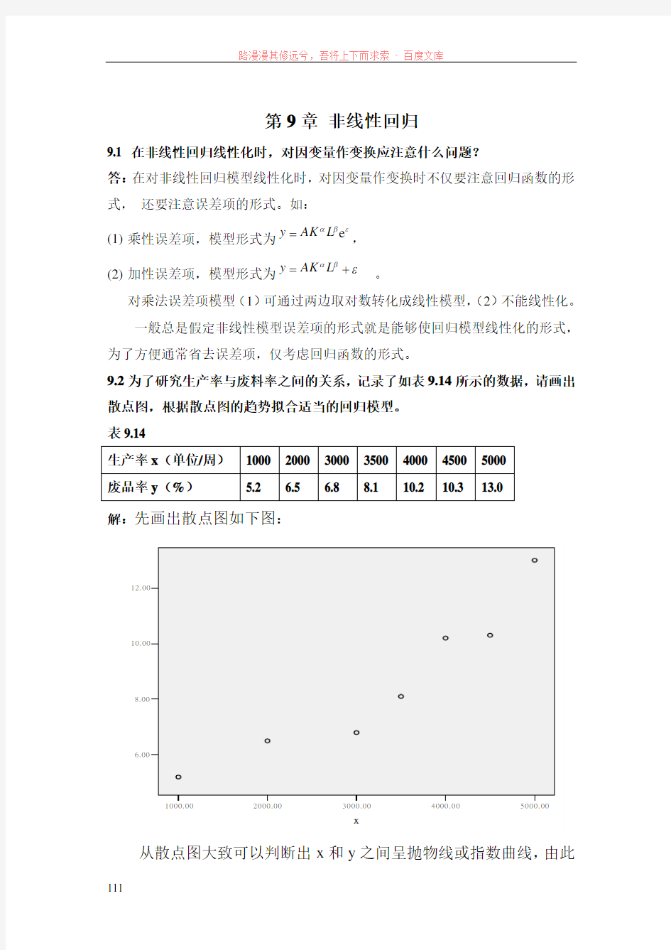
9.2为了研究生产率与废料率之间的关系，记录了如表9.14所示的数据，请画出散点图，根据散点图的趋势拟合适当的回归模型。 表9.14

生产率x （单位/周） 1000 2000 3000 3500 4000 4500 5000 废品率y （%）

5.2

6.5

6.8

8.1

10.2 10.3 13.0

解：先画出散点图如下图：

5000.00

4000.003000.002000.001000.00x

12.00

10.00

8.006.00

y

从散点图大致可以判断出x 和y 之间呈抛物线或指数曲线，由此

采用二次方程式和指数函数进行曲线回归。 （1）二次曲线 SPSS 输出结果如下：

Mode l Sum mary

.981

.962

.942

.651

R R Square

Adjusted R Square

Std. E rror of the E stim ate

The independent variable is x.

ANOVA

42.571221.28650.160.001

1.6974.424

44.269

6

Regression Residual Total

Sum of Squares df

Mean Square

F Sig.The independent variable is x.

Coe fficients

-.001.001-.449-.891.4234.47E -007.000

1.417

2.812.0485.843 1.324

4.414.012

x x ** 2

(Constant)

B Std. E rror Unstandardized Coefficients Beta

Standardized

Coefficients

t

Sig.从上表可以得到回归方程为：72? 5.8430.087 4.4710y

x x -=-+? 由x 的系数检验P 值大于0.05，得到x 的系数未通过显著性检验。 由x 2的系数检验P 值小于0.05，得到x 2的系数通过了显著性检验。 （2）指数曲线

Mode l Sum mary

.970

.941

.929

.085

R

R Square

Adjusted R Square

Std. E rror of the E stim ate

The independent variable is x.

ANOVA

.5731.57379.538

.000

.0365.007

.609

6

Regression Residual Total

Sum of Squares

df

Mean Square

F Sig.The independent variable is x.

Coe fficients

.000.000.970

8.918.0004.003.348

11.514.000

x

(Constant)

B Std. E rror Unstandardized Coefficients Beta

Standardized

Coefficients

t

Sig.The dependent variable is ln(y).

从上表可以得到回归方程为：0.0002t ? 4.003y

e 由参数检验P 值≈0<0.05，得到回归方程的参数都非常显著。

从R 2值，σ的估计值和模型检验统计量F 值、t 值及拟合图综合考虑，

指数拟合效果更好一些。

9.3 已知变量x与y的样本数据如表9.15，画出散点图，试用αeβ/x来拟合回归模型，假设：

(1)乘性误差项，模型形式为y=αeβ/x eε

(2)加性误差项，模型形式为y=αeβ/x+ε。

表9.15

序号x y 序号x y 序号x y

1 4.20 0.086 6 3.20 0.150 11 2.20 0.350

2 4.06 0.090 7 3.00 0.170 12 2.00 0.440

3 3.80 0.100 8 2.80 0.190 13 1.80 0.620

4 3.60 0.120 9 2.60 0.220 14 1.60 0.940

5 3.40 0.130 10 2.40 0.240 15 1.40 1.620

解：散点图：

(1) 乘性误差项，模型形式为y=αe β/x e ε

线性化：lny=ln α+β/x +ε 令y1=lny, a=ln α,x1=1/x . 做y1与x1的线性回归，SPSS 输出结果如下：

Model Summ ary

b

.999a .997

.997.04783

Model 1R

R Square

Adjusted R Square

Std. E rror of the Estimate

P redictors: (Constant), x1a. Dependent Variable: y1

b. ANOVA b

10.930110.9304778.305

.000a

.03013.002

10.960

14

Regression Residual Total

Model 1

Sum of Squares df

Mean Square

F Sig.P redictors: (Constant), x1a. Dependent Variable: y1

b. Coe fficients

a -3.856.037-103.830.0006.080.088

.999

69.125.000

(Constant)x1

Model

1

B Std. E rror Unstandardized Coefficients Beta

Standardized

Coefficients

t

Sig.Dependent Variable: y1

a.

从以上结果可以得到回归方程为：y1=-3.856+6.08x1

F 检验和t 检验的P 值≈0<0.05，得到回归方程及其参数都非常显著。

回代为原方程为：y=0.021e 6.08/x （2）加性误差项，模型形式为y=αe

β/x

+ε

不能线性化，直接非线性拟合。给初值α=0.021，β=6.08（线性化结果），NLS 结果如下：

Parameter E stimates

.021.001.020.023

6.061.044 5.965 6.157

P aram eter

a

b

E stim ate Std. E rror Low er Bound Upper Bound

95% Confidence I nterval

ANOVA a

4.4582 2.229

.00113.000

4.45915

2.46714

Source

Regression

Residual

Uncorrected Total

Corrected Total

Sum of

Squares df

Mean

Squares

Dependent variable: y

R squared = 1 - (Residual Sum of Squares) /

(Corrected Sum of Squares) = 1.000.

a.

从以上结果可以得到回归方程为：y=0.021e6.061/x

根据R2≈1，参数的区间估计不包括零点且较短，可知回归方程拟合非常好，且其参数都显著。

9.4 Logistic 回归函数常用于拟合某种消费品的拥有率，表8.17（书上239页，此处略）是北京市每百户家庭平均拥有的照相机数，试针对以下两种情况拟合Logistic 回归函数。

0111

t y b b u

=

+

（1）已知100u =，用线性化方法拟合，

（2）u 未知，用非线性最小二乘法拟合。根据经济学的意义知道，u 是拥有率的上限，初值可取100；b0>0,0

解：（1），100u =时，的线性拟合。对0111

t y b b u

=

+函数线性化得到：

11ln() 1.8510.264100y -=--0111ln()ln ln 100b t b y -=+，令311ln()100

y y =-，作3

y 关于t 的线性回归分析，SPSS 输出结果如下：

Model Summ ary

b

.994a .988

.987.16820

Model 1R

R Square

Adjusted R Square

Std. E rror of the Estimate

P redictors: (Constant), t a. Dependent Variable: y3

b.

ANOVA b

39.839139.8391408.165.000a

.48117.028

40.320

18

Regression Residual Total

Model 1

Sum of Squares df

Mean Square

F Sig.P redictors: (Constant), t a. Dependent Variable: y3

b.

Coe fficients

a -1.851.080-23.039.000-.264.007

-.994

-37.526.000

(Constant)t

Model

1

B Std. E rror Unstandardized Coefficients Beta

Standardized

Coefficients

t

Sig.Dependent Variable: y3

a.

由表Model Summary 得到，0.994R =趋于1，回归方程的拟合优度好，由表ANOVA 得到回归方程显著，由Coefficients 表得到，回归系数都是显著的，得到方程：11

ln() 1.8510.264100

y -

=--，进一步计算得到：00.157b =，10.768b =（100u =）

回代变量得到最终方程形式为： 1

?0.010.1570.768t

y

=+?

最后看拟合效果，通过sequence 画图：

由图可知回归效果比较令人满意。

（2）非线性最小二乘拟合,取初值100u =,00.157b =,10.768b =： 一共循环迭代8次，得到回归分析结果为：

Parameter E stimates

91.062 2.03586.74795.377.211.028.152.271.727.012

.701.753

P aram eter

u b c E stim ate Std. E rror

Low er Bound Upper Bound

95% Confidence I nterval

ANOVA a

60774.331320258.11085.36916 5.33660859.7001915690.386

18

Source Regression Residual Uncorrected Total Corrected Total Sum of

Squares df Mean

Squares

Dependent variable: y

R squared = 1 - (Residual Sum of Squares) /(Corrected Sum of Squares) = .995.

a.

0.995R =>0.994，得到回归效果比线性拟合要好，且：91.062u =，

00.211b =，10.727b =，

回归方程为：1

1

0.211*0.72791.062

t

y =

+。

最后看拟合效果，由sequence 画图：

得到回归效果很好，而且较优于线性回归。

9.5表9.17（书上233页，此处略）数据中GDP 和投资额K 都是用定基居民消费价格指数（CPI ）缩减后的，以1978年的价格指数为100。 （1） 用线性化乘性误差项模型拟合C-D 生产函数；

（2） 用非线性最小二乘拟合加性误差项模型的C-D 生产函数； （3） 对线性化检验自相关，如果存在自相关则用自回归方法改进； （4） 对线性化检验多重共线性，如果存在多重共线性则用岭回归方法改进；

解：（1）对乘法误差项模型可通过两边取对数转化成线性模型。

ln y =ln A + α ln K + β ln L

令y ′=ln y ,β0=ln A ,x 1=ln K ,x 2=ln L ,则转化为线性回归方程：

y ′=β0+ α x 1+ β

x 2+ ε

SPSS 输出结果如下：

模型综述表

Model Summ ary

b

.997a .994

.993.04836

Model 1R

R Square

Adjusted R Square

Std. E rror of the Estimate

P redictors: (Constant), lnL, lnK a. Dependent Variable: lnY

b.

从模型综述表中可以看到，调整后的

为0.993，说明C-D 生产函数拟合效

果很好，也说明GDP 的增长是一个指数模型。

方差分析表

ANOVA b

8.4462 4.2231805.601

.000a

.05122.002

8.497

24

Regression Residual Total

Model 1

Sum of Squares

df

Mean Square

F Sig.P redictors: (Constant), lnL, lnK

a. Dependent Variable: lnY

b.

从方差分析表中可以看到，F 值很大，P 值为零，说明模型通过了检验，这与上述分析结果一致。

系数表

Coe fficients a

-1.785 1.438-1.241.228

.801.056.86114.370.000

.402.171.141 2.354.028 (Constant)

lnK

lnL

Model

1

B Std. E rror

Unstandardized

Coefficients

Beta

Standardized

Coefficients

t Sig.

Dependent Variable: lnY

a.

根据系数表显示，回归方程为：

尽管模型通过了检验，但是也可以看到，常数项没有通过检验，但在这个模型里，当lnK和lnL都为零时，lnY为-1.785，即当K和L都为1时，GDP为0.168，也就是说当投入资本和劳动力都为1个单位时，GDP将增加0.168个单位，这种解释在我们的承受范围内，可以认为模型可以用。

最终方程结果为：

y=0.618K0.801 L0.404

（2）用非线性最小二乘法拟合加性误差项模型的C-D生产函数；

上述假设误差是乘性的，现假设误差是加性的情况下使用非线性最小二乘法估计。初值采用（1）中参数的结果，SPSS输出结果如下：

参数估计表

Parameter E stimates

.407.885-1.429 2.243

.868.066.731 1.006

.270.243-.234.774

P aram eter

P

a

b

E stim ate Std. E rror Low er Bound Upper Bound

95% Confidence I nterval

SPSS经过多步迭代，最终得到的稳定参数值为P=0.407，a=0.868，b=0.270

y=0.407K0.868 L0.270

为了比较这两个方程，我们观察下面两个图

线性回归估计拟合曲线图

非线性最小二乘估计拟合曲线图

我们知道，乘性误差相当于是异方差的，做了对数变换后，乘性误差转为加性误差，这种情况下认为方差是相等的，那么第一种情况（对数变换线性化）就大大低估了GDP 数值大的项，因此，它对GDP 前期拟合的很好，而在后期偏差就变大了，同时也会受到自变量之间的自相关和多重共线性的综合影响；非线性最小二乘法完全依赖数据，如果自变量之间存在比较严重的异方差、自相关以及多重共线性，将对拟合结果造成很大的影响。因此，不排除异方差、自相关以及多重共线性的存在。

（3） 对线性化回归模型采用DW 检验自相关，结果如下：

模型综述表

Model Summ ary

b

.997a .994

.993.04836.715

Model 1R

R Square

Adjusted R Square

Std. E rror of the Estimate

Durbin-Watson

P redictors: (Constant), lnL, lnK a. Dependent Variable: lnY

b. DW=0.715<1.27，落在自相关的区间，所以采用迭代法改进

将得到的数据再取对数，而后用普通最小二乘法估计，保留DW 值

模型综述表

Model Summ ary

b

.983a .967

.964478.90271 1.618

Model 1R

R Square

Adjusted R Square

Std. E rror of the Estimate Durbin-Watson

P redictors: (Constant), Ltt, Ktt a. Dependent Variable: Ytt

b.

方差分析表

ANOVA b

7.5542 3.777601.286.000a

.13221.006

7.686

23

Regression Residual Total

Model 1

Sum of Squares

df

Mean Square

F Sig.P redictors: (Constant), lnLtt, lnKtt a. Dependent Variable: lnYtt

b.

系数表

Coe fficients

a

-1.859 1.470-1.265.220.755.054.85214.098.000.465.180

.156

2.577.018

(Constant)lnKtt lnLtt

Model 1

B Std. E rror Unstandardized Coefficients Beta

Standardized

Coefficients

t

Sig.Dependent Variable: lnYtt

a.

从模型综述表中可以看到，DW=1.618>1.45，认为消除了自相关；方差分析

表中可以看到F值很大，P值为零，说明模型通过了检验。

从系数表可得回归方程：

再迭代回去，最终得方程为：

Lny t－Lny t－１＝-1.859＋0.755(LnK t－LnK t－１) ＋0.465(LnL t－LnL t－１)

（4）对线性化回归方程通过VIF检验多重共线性：

方差分析表

ANOVA b

8.4462 4.2231805.601.000a

.05122.002

8.49724

Regression

Residual

Total

Model

1

Sum of

Squares df Mean Square F Sig.

P redictors: (Constant), lnL, lnK

a.

Dependent Variable: lnY

b.

系数表

Coefficients a

-1.785 1.438-1.241.228

.801.056.86114.370.000.07713.034

.402.171.141 2.354.028.07713.034 (Constant)

lnK

lnL

Model

1

B Std. E rror

Unstandardized

Coefficients

Beta

Standardized

Coefficients

t Sig.Tolerance VI F

Collinearity Statistics Dependent Variable: lnY

a.

多重共线性诊断表

Colline arity Diagnostics a

2.997 1.000.00.00.00

.00330.539.00.09.00

1.63E-005429.012 1.00.91 1.00

Dimension

1

2

3

Model

1

E igenvalue

Condition

I ndex(Constant)lnK lnL

Variance P roportions

Dependent Variable: lnY

a.

直观法：从模型综述表上可以看到，F值很大，而t值很小，这是多重共线性造成的影响；

VIF检验法：从系数表上可以看到，VIF=13>10，也说明多重共线性的存在；条件数：从诊断表上可以看到，最大的条件数是429，远远大于了100，所以自变量之间存在较为严重的多重共线性。

利用岭回归改进：

R-SQUARE AND BETA COEFFICIENTS FOR ESTIMATED VALUES OF K

K RSQ LNK LNL

______ ______ ________ ________

.00000 .99394 .860706 .141014

.05000 .99015 .646381 .330432

.10000 .98639 .577758 .375355

.15000 .98260 .539715 .390822

.20000 .97843 .513383 .395623

.25000 .97379 .492922 .395526

.30000 .96869 .475918 .392882

.35000 .96318 .461184 .388818

.40000 .95730 .448063 .383937

.45000 .95109 .436158 .378587

.50000 .94462 .425211 .372979

.55000 .93791 .415047 .367248

.60000 .93101 .405541 .361481

.65000 .92395 .396598 .355735

.70000 .91677 .388147 .350049

从岭迹图观察，当k=0.2时，变量基本趋于稳定

取k=0.2进行岭回归，SPSS输出结果为：α=0.479，β=1.127

从岭回归给出的结果来看，说明劳动力L较资金K对GDP的影响较大，而我国属于人口大国，就业人数对GDP的贡献不一定有显著的影响，相反，资金对GDP的影响按常理来说是非常显著的，这点普通最小二乘法给出了合理的解释，但是，岭回归在理论上很可信的。总之，影响统计的因素有很多，例如统计员的失误、国家政策等，造成函数系数的不稳定。