正态分布推导

正态分布的概率密度函数的推导

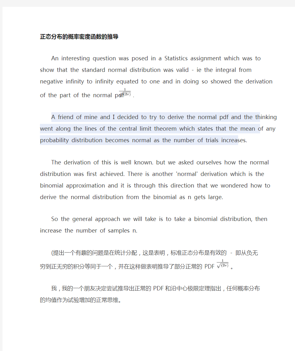
An interesting question was posed in a Statistics assignment which was to show that the standard normal distribution was valid - ie the integral from negative infinity to infinity equated to

one and in doing so showed the derivation of the part of the normal pdf.

A friend of mine and I decided to try to derive the normal pdf and the thinking went along the lines of the central limit theorem which states that the mean of any probability distribution becomes normal as the number of trials increases.

The derivation of this is well known.but we asked ourselves how the normal distribution was first achieved.There is another 'normal' derivation which is the binomial approximation and it is through this direction that we wondered how to derive the normal distribution from the binomial as n gets large.

So the general approach we will take is to take a binomial distribution, then increase the number of samples n.

(提出一个有趣的问题是在统计分配，这是表明，标准正态分布是有效的 - 即从负无穷到正无穷的积分等同于一个，并在这样做表明推导了部分正常的PDF 。

我，我的一个朋友决定尝试推导出正常的PDF和沿中心极限定理指出，任何概率分布的均值作为试验增加的正常思维。

这个推导是众所周知的。但我们问自己如何正态分布首次实现。有另一种“正常”的推导，这是二项式近似和它是通过这个方向，我们想知道如何从二项式正态分布为n变大。

因此，我们将采取的一般方法是一个二项分布，再增加样本N.的数量)

Once we have done this, instead of using the horizontal lines of the distribution histogram (which would be the normal probability mass function of the binomial), we are going to 'draw' a line through each central point.

(一旦我们已经做了，而不是使用分布直方图（这将是正常的概率质量函数二项式）水平线，，我们要“画一条线”，通过每一个中心点。)

Notice how the 'probability mass function' shown in blue now extends from point through to the point.This probability mass function now represented by the blue line now looks more like a probability density function.Instead of labeling the histogram bars 1,2,3,4,5 we are instead going to label the intervals 0k, 1k, 2k, ..., nk.

(请注意显示在蓝色的“概率密度函数”，现在又延伸点到点。现在蓝线代表这概率密度函数现在看起来更像是一个概率密度函数。标签1,2,3,4,5直方图酒吧我们，而不是将标签的时间间隔0K，1K，2K，... ，NK。)

So we begin by stating our distribution as P(y) where y is the probability of an occurence of rk.From the original binomial distribution, we can immediately see that the mean

is and the variance(where p is the probability of success and q is the probability of failure).

(因此，我们首先说明我们的P（Y），其中y是RK发生的概率分布。从最初的二项分布，我们马上就可以看到，意思是和方差（其中p是成功的概率和Q是失败的概率）)。

让我们调用这个方程A

而是让variate y，这表示二项分布，考虑一个新的variate X的代表二项分布，但0为中心左右。为了实现这一目标，我们必须从每个值减去平均。

整合双方：

我们乘上一个一个，但现在的工作是什么使有效的公式是PDF。我们整合范围负到正无穷大的结果集计算A值

现在这是一个有效的概率密度函数，然后积分到必须等于。

求解与替代：

日期：

现在，我们可以写为正常分布的PDF全文：

但是，仔细考虑，这是没有完成。请记住，我们说，我们将“正常化”Y，并考虑有关平均值为中心的新variate X。所以记住，我们本质上说，，然后正态分布（Y）的PDF全文如下，并在其最常见的的形式：

（素材和资料部分来自网络，供参考。可复制、编制，期待您的好评与关注）