a new mathematical model for relative quantification real-time rt-PCR

?2001Oxford University Press Nucleic Acids Research,2001,Vol.29,No.900 A new mathematical model for relative quantification in real-time RT–PCR

Michael W.Pfaffl*

Institute of Physiology,FML-Weihenstephan,Center of Life and Food Sciences,Technical University of Munich, Germany

Received December18,2000;Revised February21,2001;Accepted March14,2001

ABSTRACT

Use of the real-time polymerase chain reaction(PCR) to amplify cDNA products reverse transcribed from mRNA is on the way to becoming a routine tool in molecular biology to study low abundance gene expression.Real-time PCR is easy to perform, provides the necessary accuracy and produces reli-able as well as rapid quantification results.But accu-rate quantification of nucleic acids requires a reproducible methodology and an adequate mathe-matical model for data analysis.This study enters into the particular topics of the relative quantification in real-time RT–PCR of a target gene transcript in comparison to a reference gene transcript.There-fore,a new mathematical model is presented.The relative expression ratio is calculated only from the real-time PCR efficiencies and the crossing point deviation of an unknown sample versus a control. This model needs no calibration curve.Control levels were included in the model to standardise each reac-tion run with respect to RNA integrity,sample loading and inter-PCR variations.High accuracy and reproducibility(<2.5%variation)were reached in LightCycler PCR using the established mathematical model.

INTRODUCTION

Reverse transcription(RT)followed by the polymerase chain reaction(PCR)is the technique of choice to analyse mRNA expression derived from various sources.Real-time RT–PCR is highly sensitive and allows quantification of rare transcripts and small changes in gene expression.As well as this,it is easy to perform,provides the necessary accuracy and produces reliable as well as rapid quantification results.The simplest detection technique for newly synthesised PCR products in real-time PCR uses SYBR Green I fluorescence dye that binds specifically to the minor groove double-stranded DNA(1).The quantification method of choice depends on the target sequence,the expected range of mRNA amount present in the tissue,the degree of accuracy required and whether quantifica-tion needs to be relative or absolute(2).Generally two quanti-fication types in real-time RT-PCR are possible.(i)A relative quantification based on the relative expression of a target gene versus a reference gene.To investigate the physiological changes in gene expression,the relative expression ratio is adequate for the most purposes.(ii)An absolute quantification, based either on an internal or an external calibration curve (1,3).Using such a calibration curve,the methodology has to be highly validated and the identical LightCycler PCR amplifi-cation efficiencies for standard material and target cDNA must be confirmed(4–6).Nevertheless,the generation of stable and reliable standard material,either recombinant DNA or recom-binant RNA,is very time consuming and it must be precisely quantified(2,7,8).Furthermore,a normalisation of the target gene with an endogenous standard is recommended.Therefore, mainly non-regulated reference genes or housekeeping genes like glyceraldehyde-3-phosphate dehydrogenase(G3PDH or GAPDH),albumin,actins,tubulins,cyclophilin,18S rRNA or 28S rRNA(9)were applicable.Housekeeping genes are present in all nucleated cell types since they are necessary for basis cell survival.The mRNA synthesis of these genes is considered to be stable and secure in various tissues,even under experimental treatments(9–11).But numerous studies have already shown that the housekeeping genes are regulated and vary under experimental conditions(12–15).To circum-vent the high expenditure of design and production of standard material,as well as optimisation and validation of a calibration curve based quantification model,and finally the need for normalisation of the target transcripts to an endogenous house-keeping transcript,a reliable and accurate relative quantifica-tion model in real-time RT–PCR is needed.

This study enters into the particular topics of the relative quantification of a target gene in comparison to a reference gene.A new and simple mathematical model for data analysis was established,the application of the new model was tested and compared with available mathematical calculation models. Derived reproducibility,based on intra-and inter-test variation of this relative quantification and accuracy of the model will be discussed.

MATERIALS AND METHODS

RNA source,total RNA extraction and RT

RNA extraction was performed as described previously(16)in bacterial Escherichia coli culture grown either in M9minimal

*To whom correspondence should be addressed at present address:Institut für Physiologie,Weihenstephaner Berg3,85354Freising,Weihenstephan,Germany. Tel:+498161713511;Fax:+498161714204;Email:pfaffl@weihenstephan.de

Nucleic Acids Research,2001,Vol.29,No.900

P AGE 2003OF 2007

media (sample preparation)or LB rich media (control prepara-tion),both with 0.4%glucose concentration (17).RNA integrity was electrophoretically verified by ethidium bromide staining and by OD 260/OD 280nm absorption ratio >1.95.Escherichia coli total RNA (1μg)was reverse transcribed with 100U of Superscript II Plus RNase H –Reverse Trancriptase (Gibco BRL Life Technologies,Gaithersburg,MD)using 100μM random hexamer primers (Pharmacia Biotech,Uppsala,Sweden)according to the manufacturer’s instructions.Optimisation of RT–PCR

Highly purified salt-free primer for target gene1(TyrA,tryptophan operon:forward primer,AAG CGT CTG GAA CTG GTT GC;reverse primer,AAA CGC TGT GCG TAA TCG CC),target gene 2(PyrB,aspartate transcarbamylase:forward primer,GCT CCA ACC AAC ATC CGA;reverse primer,TTC ACG TTG GCG TAC TCG G)and reference gene (Gst,glutathione transferase:forward primer,CTT TGC CGT TAA CCC TAA GGG;reverse primer,GCT GCA ATG TGC TCT AAC CC)were generated (MWG Biotech,Ebersberg,Germany)and optimised to an equal annealing temperature of 60°C.Condi-tions for all PCRs were optimised in a gradient cycler (Master-cycler Gradient,Eppendorf,Germany)with regard to Taq DNA polymerase (Roche Diagnostics,Basel,Switzerland),forward and reverse primers,MgCl 2concentrations (Roche Diagnostics),dNTP concentrations (Roche Diagnostics)and various annealing temperatures (55–65°C).RT–PCR amplification products were separated on a 4%high resolution NuSieve agarose (FMC Bio Products,Rockland,ME)gel electro-phoresis and analysed with the Image Master system (Pharmacia Biotech).Optimised results were transferred on the following LightCycler PCR protocol.LightCycler real-time PCR

For LightCycler reaction a mastermix of the following reaction components was prepared to the indicated end-concentration:13μl water,2.4μl MgCl 2(4mM),0.8μl forward primer (0.4μM),0.8μl reverse primer (0.4μM)and 2.0μl LightCyler (Fast Start DNA Master SYBR Green I;Roche Diagnostics).LightCycler mastermix (19μl)was filled in the LightCycler glass capillaries and 1μl cDNA (3.2,4.0,4.8,16,20or 24ng reverse transcribed total RNA)was added as PCR template.Capillaries were closed,centrifuged and placed into the Light-

Cycler rotor.The following LightCycler experimental run protocol was used:denaturation program (95°C for 10min),amplification and quantification program repeated 40times (95°C for 15s,60°C for 10s,72°C for 60s with a single fluorescence measurement),melting curve program (60–95°C with a heating rate of 0.1°C per second and a continuous fluo-rescence measurement)and finally a cooling step to 40°C.For the mathematical model it is necessary to determine the crossing points (CP)for each transcript.CP is defined as the point at which the fluorescence rises appreciably above the background fluorescence.‘Fit Point Method’must be performed in the LightCycler software 3.3(Roche Diagnostics),at which CP will be measured at constant fluorescence level (18).RESULTS

Confirmation of primer specificity

Specificity of RT–PCR products was documented with high resolution gel electrophoresis and resulted in a single product with the desired length (TyrA,978bp;PyrB,530bp;and Gst,

Table 1.Intra-assay (test precision)and inter-assay variation (test variability)of LightCycler real-time RT–PCR

Determination of variation was done in 20ng reverse transcribed total RNA.Test variation is based on CP variation and expressed as mean CP with CV.

Intra-assay variation (n =3)Inter-assay variation (n =3)Mean CP

CV Mean CP CV TyrA (sample)15.0200.06%15.311 3.58%TyrA (control)20.3030.09%20.426 2.98%PyrB (sample)16.031 2.16%16.289 3.91%PyrB (control)11.720 1.32%12.011 3.18%Gst (sample)14.5330.65%14.371 2.26%Gst (control)

14.277

0.11%

13.997

2.62%

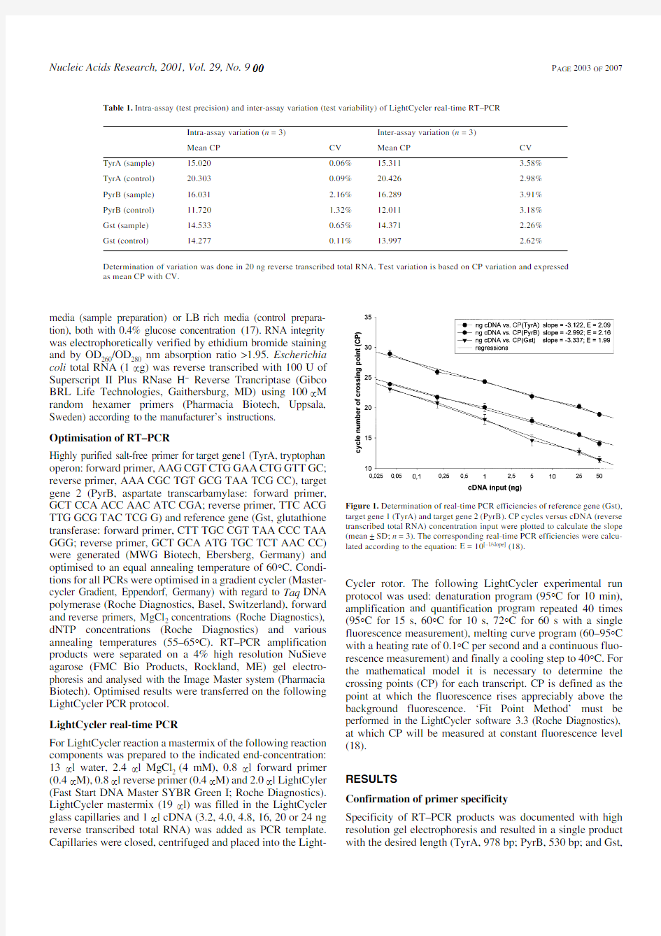
Figure 1.Determination of real-time PCR efficiencies of reference gene (Gst),target gene 1(TyrA)and target gene 2(PyrB).CP cycles versus cDNA (reverse transcribed total RNA)concentration input were plotted to calculate the slope (mean ±SD;n =3).The corresponding real-time PCR efficiencies were calcu-lated according to the equation:E =10[–1/slope](18).

P AGE2004OF200700Nucleic Acids Research,2001,Vol.29,No.9 402bp).In addition a LightCycler melting curve analysis was

performed which resulted in single product specific melting

temperatures as follows:TyrA,89.6°C;PyrB,88.5°C;and Gst,

88.3°C.No primer-dimers were generated during the applied40

real-time PCR amplification cycles.

Real-time PCR amplification efficiencies and linearity

Real-time PCR efficiencies were calculated from the given

slopes in LightCycler software.The corresponding real-time

PCR efficiency(E)of one cycle in the exponential phase was

calculated according to the equation:E=10[–1/slope](Fig.1)(18).

Investigated transcripts showed high real-time PCR efficiency

rates;for TyrA,2.09;PyrB,2.16;and Gst,1.99in the investi-

gated range from0.40to50ng cDNA input(n=3)with high

linearity(Pearson correlation coefficient r>0.95).

Intra-and inter-assay variation

To confirm accuracy and reproducibility of real-time PCR the

intra-assay precision was determined in three repeats within

one LightCycler run.Inter-assay variation was investigated in

three different experimental runs performed on3days using

three different premix cups of LightCycler,Fast Start DNA Master SYBR Green I kit(Roche Diagnostics).Determination of variation was done in20ng transcribed total RNA(Table1). Test reproducibility for all investigated transcripts was low in inter-test experiments(<3.91%)and even lower in intra-test experiments(<2.16%).The calculation of test precision and test variability is based on the CP variation from the CP mean value.

Mathematical model for relative quantification in real-time PCR

A new mathematical model was presented to determine the relative quantification of a target gene in comparison to a refer-ence gene.The relative expression ratio(R)of a target gene is calculated based on E and the CP deviation of an unknown sample versus a control,and expressed in comparison to a reference gene.

1 Equation1shows a mathematical model of relative expression ratio in real-time PCR.The ratio of a target gene is expressed in a sample versus a control in comparison to a reference gene.

E target is the real-time PCR efficiency of target gene transcript;

E ref is the real-time PCR efficiency of a reference gene tran-script;?CP target is the CP deviation of control–sample of the target gene transcript;?CP ref=CP deviation of control–sample of reference gene transcript.The reference gene could be a stable and secure unregulated transcript,e.g.a house-keeping gene transcript.For the calculation of R,the individual real-time PCR efficiencies and the CD deviation(?CP)of the investigated transcripts must be known.Real-time PCR efficiencies were calculated,according to E=10[–1/slope](18),as shown in Figure1.CP deviations of control cDNA minus sample of the target gene and reference genes were calculated according to the derived CP values.Mean CP,variation of CP and?CP values between control and sample of investigated transcripts are listed in Table2.The influence of differing cDNA input concentrations on?CP are also shown.Intended cDNA input concentration variation of control and sample were compared at different levels(low level,3.2,4.0,4.8ng cDNA;high level,16,20and24ng cDNA).They resulted in stable and constant?CP cycle numbers.In Table3the corre-sponding ratios of target genes in comparison to the reference gene were calculated,through to the established mathematical model(equation1).The expression ratios of target genes remain stable,even under intended±20%cDNA variation and low and high cDNA input levels,performed in two runs.A minimal coefficient of variation(CV)of2.50and1.74%was observed,respectively.

Regulation of investigated gene transcripts

All investigated transcript expressions were regulated diver-gently(Table3).The expression of Gst was constant,inde-pendent of media conditions,and therefore was chosen as endogenous standard or reference gene transcript Fig.2.TyrA mRNA expression,measured in20ng cDNA,was up-regulated 49.1-fold(2.095.283)in M9minimal compared to LB rich medium under high cDNA input conditions.Under the considera-tion of the reference gene expression the real up-regulation ratio was,on average,58.5-fold.PyrB mRNA expression was down-regulated under M9minimal medium conditions by a factor of27.6(2.164.311).With the normalisation of the endog-enous standard transcript,the exact relative expression ratio can be calculated to23.2.

DISCUSSION

RT followed by PCR is the most powerful tool to amplify small amounts of mRNA(19).Because of its high ramping rates,limited annealing and elongation time,the rapid cycle PCR in the LightCycler system offers stringent reaction condi-tions to all PCR components and leads to a primer sensitive and template specific PCR(20).The application of fluo-rescence techniques to real-time PCR combines the PCR amplification,product detection and quantification of newly synthesised DNA,as well as verification in the melting curve analysis.This led to the development of new kinetic RT–PCR

ratio=

E target

()?CP target control sample

–

()

E ref

()?CP ref control sample

–

()

-------------------------------------------------------------------

-

Figure2.Real-time RT–PCR SYBR Green I fluorescence history versus cycle

number of target gene1(TyrA),target gene2(PyrB)and reference gene(Gst)

in sample cDNA and control cDNA.CP determination was done at fluores-

cence level1.

Nucleic Acids Research,2001,Vol.29,No.900

P AGE 2005OF 2007

methodologies that are revolutionising the possibilities of mRNA quantification (21).

In this paper,we focused on the relative quantification of target gene transcripts in comparison to a reference gene tran-script.A new mathematical model for data analysis was presented to calculate the relative expression ratio on the basis of the PCR efficiency and crossing point deviation of the investigated transcripts (equation 1).The concept of threshold fluorescence is the basis of an accurate and reproducible quan-tification using fluorescence-based RT–PCR methods (22).Threshold fluorescence is defined as the point at which the fluorescence rises appreciably above the background fluores-cence.In the Fit Point Method,the threshold fluorescence and therefore the DNA amount in the capillaries is identical for all samples.CP determination with the ‘Second Derivative Maximum Method’is not adequate for our mathematical model,because quantification is done at the point of most effi-cient real-time PCR where the second derivative is at its maximum (18).

A linear relationship between the CP,crossing the threshold fluorescence,and the log of the start molecules input in the reaction is given (18,23).Therefore,quantification will always occur during the exponential phase,and it will not be affected by any reaction components becoming limited in the plateau phase (7).In the established model the relative expression ratio

of a target gene is normalised with the expression of an endo-genous desirable unregulated reference gene transcript to compensate inter-PCR variations between the runs.The CP of the chosen reference gene is the same in the control and the sample (?CP =0).Stable and constant reference gene mRNA levels are given.Under these considerations of an unregulated reference gene transcript,no normalisation is needed and equa-tion 1can be shortened to equation 2.

2

Equation 2shows a mathematical model of relative expression ratio in real-time PCR under constant reference gene expression.CP values in the sample and control are equal and represent ideal housekeeping conditions (?CP ref =0,E ref =1).

Two other mathematical models are available for the relative quantification during real-time PCR.The ‘efficiency calibrated mathematical method for the relative expression ratio in real-time PCR’is presented by Roche Diagnostics in a truncated form in an internal publication (24).The complete equation is,

Table 2.Mean CP and CV of target gene 1(TyrA)and target gene 2(PyrB)in comparison to intended

concentration variation of reference gene (Gst)low level (3.2,4.0and 4.8ng per capillary)and high level cDNA input (16,20and 24ng)

cDNA input (ng)

Mean CP (n =3)

CV (%)

?CP (cycles)

High cDNA input level TyrA (sample)2015.0200.06+5.283

TyrA (control)2020.3030.09PyrB (sample)2016.031 2.16–4.311PyrB (control)2011.720 1.32Gst (sample)1614.2900.73–0.277Gst (control)1614.0130.39Gst (sample)2014.5330.65–0.256Gst (control)2014.2770.11Gst (sample)2414.957 1.29–0.227Gst (control)24

14.730

1.14

Low cDNA input level TyrA (sample) 4.017.353 2.16+5.487

TyrA (control) 4.022.840 1.26PyrB (sample) 4.017.6670.75–4.277PyrB (control) 4.013.3900.12Gst (sample) 3.216.9270.643–0.050Gst (control) 3.216.877 1.81Gst (sample) 4.016.750 2.31–0.127Gst (control) 4.016.623 1.04Gst (sample) 4.816.297 1.68–0.077Gst (control)

4.8

16.220

0.69

ratio =E target ()

?CP target control -sample )

(E ref ()0

------------------------------------------------------------------ratio =E target ()

?CP target control -sample ()

P AGE 2006OF 2007

00Nucleic Acids Research,2001,Vol.29,No.9

in principle,the same and the results are in identical relative expression ratio like our model (equation 3).

3

Efficiency calibrated mathematical method for the relative

expression ratio in real-time PCR presented by Soong et al.(24).But the method of calculation in the described mathematical model is hard to understand.The second model available,the ‘Delta–delta method’for comparing relative expression results between treatments in real-time PCR (equation 4)is presented by PE Applied Biosystems (Perkin Elmer,Forster City,CA).4

Equation 4shows a mathematical delta–delta method for comparing relative expression results between treatments in real-time PCR developed by PE Applied Biosystems (Perkin Elmer).Optimal and identical real-time amplification efficiencies of target and reference gene of E =2are presumed.The delta–delta method is only applicable for a quick estima-tion of the relative expression ratio.For such a quick estima-tion,equation 1can be shortened and transferred into equation 4,under the condition that E target =E ref =2.Our presented formula combines both models in order to better understand the mode of CP data analysis and for a more reliable and exact relative gene expression.

Relative quantification is always based on a reference tran-script.Normalisation of the target gene with an endogenous standard was done via the reference gene expression,to compensate inter-PCR variations.Beside this further control levels were included in the mathematical model to standardise each reaction run with respect to RNA integrity,RT efficiency or cDNA sample loading variations.The reproducibility of the RT step varies greatly between tissues,the applied RT isola-tion methodology (25)and the RT enzymes used (26).Different cDNA input concentrations were tested on low and high cDNA input ranges,to mimic different RT efficiencies (±20%)at different quantification levels.In the applied two-step RT–PCR,using random hexamer primers,all possible interferences during RT will influence all target transcripts as well as the internal reference transcript in parallel.Occurring background interferences retrieved from extracted tissue components,like enzyme inhibitors,and cDNA synthesis efficiency were related to target and reference similarly.All products underwent identical reaction conditions during RT and variations only disappear during real-time PCR.Any source of error during RT will be compensated through the model itself.Widely distributed single-step RT–PCR models are not applicable,because in each reaction set-up and for each investigated factor individual and slightly different RT condi-tions will occur.Therefore,the variation in a two-step RT–PCR will always be lower,and the reproducibility of the assay will be higher,that in a single-step RT–PCR (8).Reproducibility of

the developed mathematical model was dependent on the exact determination of real-time amplification efficiencies and on the given low LightCycler CP variability.In our mathematical model the necessary reliability and reproducibility was given,which was confirmed by high accuracy and a relative error of <2.5%using low and high template concentration input.CONCLUSION

LightCycler real-time PCR using SYBR Green I fluorescence dye is a rapid and sensitive method to detect low amounts of mRNA molecules and therefore offers important physiological insights on mRNA expression level.The established mathe-matical model is presented in order to better understand the mode of analysis in relative quantification in real-time RT–PCR.It is only dependent on ?CP and amplification efficiency of the transcripts.No additional artificial nucleic acids,like recombinant nucleic acid constructs in external calibration curve models,are needed.Reproducibility of LightCycler RT–PCR in general and the minimal error rate of the model allows for an accurate determination of the relative expression ratio.Even different cDNA input resulted in minor variations.Rela-tive expression is adequate for the most relevant physiological expression changes.In future it is not necessary to establish more complex and time consuming quantification models based on calibration curves.For the differential display of mRNA the relative expression ratio is an ideal and simple tool for the verification of RNA or DNA array chip technology results.

ACKNOWLEDGEMENTS

The author thanks D.Schmidt for technical assistance.Primers,primer sequences and samples were kindly donated by Drs

ratio =E ref ()Sample

CP

E target ()Sample CP ----------------------------------÷E ref ()

Calibrator

CP

E target ()

Calibrator

CP

--------------------------------------ratio =2?CP sample -?CP control []

–ratio =2

??CP

–Table 3.Influence of variation in cDNA input (±20%)of control and sample (high and low level)on the variation in relative expression ratio based on equation 1and the error of mathematical model,expressed as CV of R Gst

TyrA PyrB E =1.99

E =2.09

E =2.16

High cDNA input level ?CP =+5.283?CP =–4.31180%cDNA input ?CP =–0.277R =59.476R =0.04375100%cDNA input ?CP =–0.256R =58.625R =0.04312120%cDNA input ?CP =–0.227R =57.459R =0.04226Mean of R 58.459000.04304Error/CV of R 1.73%

1.74%

Low cDNA input level ?CP =+5.487?CP =–4.27716%cDNA input ?CP =–0.050R =59.104R =0.0384420%cDNA input ?CP =–0.127R =62.102R =0.0403124%cDNA input DCP =–0.077R =60.208R =0.03914Mean of R 60.4710.03930Error/CV of R

2.50%

2.49%

Nucleic Acids Research,2001,Vol.29,No.900P AGE2007OF2007

S.Wegener and W.Mann in collaboration with the BioChip division of MWG Biotech in Ebersberg,Germany. REFERENCES

1.Morrison,T.,Weis,J.J.and Wittwer,C.T.(1998)Quantification of low-

copy transcripts by continuous SYBR Green I monitoring during

amplification.Biotechniques,24,954–962.

2.Freeman,W.M.,Walker,S.J.and Vrana,K.E.(1999)Quantitative RT–

PCR:pitfalls and potential.Biotechniques,26,112–122.

3.Pfaffl,M.W.(2001)Development and validation of an externally

standardised quantitative insulin like growth factor-1(IGF-1)RT–PCR using LightCycler SYBR?Green I technology.In Meuer,S.,Wittwer,C.

and Nakagawara,K.(eds),Rapid Cycle Real-time PCR,Methods and

Applications.Springer Press,Heidelberg,Germany pp.281–291.

4.Ferré,F.(1992)Quantitative or semi-quantitative PCR:reality versus

myth.PCR Methods Appl.,2,1–9.

5.Souazé,F.,Ntodou-Thomé,A.,Tran,C.Y.,Rostene,W.and Forgez,P.(1996)

Quantitative RT–PCR:limits and accuracy.Biotechniques,21,280–285.

6.Overbergh,L.,Valckx,D.,Waer,M.and Mathieu,C.(1999)Quantification

of murine cytokine mRNAs using real time quantitative reverse

transcriptase PCR.Cytokines,11,305–312.

7.Bustin,S.A.(2000)Absolute quantification of mRNA using real-time

reverse transcription polymerase chain reaction assays.J.Mol.

Endocrinol.,25,169–193.

8.Pfaffl,M.W.and Hageleit,M.(2001)Validities of mRNA quantification

using recombinant RNA and recombinant DNA external calibration

curves in real-time RT–PCR.Biotechnol.Lett.,23,275–282.

9.Marten,N.W.,Burke,E.J.,Hayden,J.M.and Straus,D.S.(1994)Effect of

amino acid limitation on the expression of19genes in rat hepatoma cells.

FASEB J.,8,538–544.

10.Foss,D.L.,Baarsch,M.J.and Murtaugh,M.P.(1998)Regulation of

hypoxanthine phosphoribosyltransferase,glyceraldehyde-3-phosphate

dehydrogenase andβ-actin mRNA expression in porcine immune cells and tissues.Anim.Biotechnol.,9,67–78.

11.Thellin,O.,Zorzi,W.,Lakaye,B.,De Borman,B.,Coumans,B.,Hennen,G.,

Grisar,T.,Igout,A.and Heinen,E.(1999)Housekeeping genes as internal standards:use and limits.J Biotechnol.,75,291–295.

12.Bhatia,P.,Taylor,W.R.,Greenberg,A.H.and Wright,J.A.(1994)Comparison

of glyceraldehyde-3-phosphate dehydrogenase and28S-ribosomal RNA gene expression as RNA loading controls for northern blot analysis of cell lines of varying malignant potential.Anal.Biochem.,216,223–226.13.Bereta,J.and Bereta,M.(1995)Stimulation of glyceraldehyde-3-phosphate

dehydrogenase mRNA levels by endogenous nitric oxide in cytokine-activated https://www.360docs.net/doc/f63134412.html,mun.,217,363–369.

14.Chang,T.J.,Juan,C.C.,Yin,P.H.,Chi,C.W.and Tsay,H.J.(1998)Up-

regulation ofβ-actin,cyclophilin and GAPDH in N1S1rat hepatoma.

Oncol.Rep.,5,469–471.

15.Zhang,J.and Snyder,S.H.(1992)Nitric oxide stimulates auto-ADP-

ribosylation of glyceraldehydes3phosphate dehydrogenase.Proc.Natl https://www.360docs.net/doc/f63134412.html,A,89,9382–9385.

16.Pfaffl,M.W.,Meyer,H.H.D.and Sauerwein,H.(1998)Quantification of

the insulin like growth factor-1mRNA:development and validation of an internally standardised competitive reverse transcription-polymerase

chain reaction.Exp.Clin.Endocrinol.Diabetes,106,502–512.

17.Maniatis,T.,Fritsch,E.F.and Sambrook,J.(1982)Molecular Cloning:A

Laboratory Manual.Cold Spring Harbor Laboratory Press,Cold Spring Harbor,NY.

18.Rasmussen,R.(2001)Quantification on the LightCycler.In Meuer,S.,

Wittwer,C.and Nakagawara,K.(eds),Rapid Cycle Real-time PCR,

Methods and Applications.Springer Press,Heidelberg,pp.21–34.

19.Wang,A.M.,Doyle,M.V.and Mark,D.F.(1989)Quantitation of mRNA by the

polymerase chain reaction.Proc.Natl https://www.360docs.net/doc/f63134412.html,A,86,9717–9721.

20.Wittwer,C.T.,Ririe,K.M.,Andrew,R.V.,David,D.A.,Gundry,R.A.and

Balis,U.J.(1997)The LightCycler:a microvolume multisample

fluorimeter with rapid temperature control.Biotechniques,22,176–181.

21.Orlando,C.,Pinzani,P.and Pazzagli,M.(1998)Developments in

quantitative https://www.360docs.net/doc/f63134412.html,b.Med.,36,255–269.

22.Higuchi,R.,Fockler,C.,Dollinger,G.and Watson,R.(1993)Kinetic PCR

analysis:real-time monitoring of DNA amplification reactions.

Biotechnology,11,1026–1030.

23.Gibson,U.E.,Heid,C.A.and Williams,P.M.(1996)A novel method for

real time quantitative RT–PCR.Genome Res.,6,995–1001.

24.Soong,R.,Ruschoff,J.and Tabiti,K.(2000)Detection of colorectal

micrometastasis by quantitative RT–PCR of cytokeratin20mRNA.

Roche Diagnostics internal publication.

25.Mannhalter,C.,Koizar,D.and Mitterbauer,G.(2000)Evaluation of RNA

isolation methods and reference genes for RT–PCR analyses of rare target https://www.360docs.net/doc/f63134412.html,b.Med.,38,171–177.

26.Wong,L.,Pearson,H.,Fletcher,A.,Marquis,C.P.and Mahler,S.(1998)

Comparison of the efficiency of M-MuLV reverse transcriptase,RNase H–M-MuLV reverse transcriptase and AMV reverse transcriptase for the amplification of human immunglobulin genes.Biotechnol.Techniques, 12,485–489.