CMB power spectrum estimation and map reconstruction with the Expectation - Maximization al

a r X i v :a s t r o -p h /0302094v 3 2 J u l 2003

Mon.Not.R.Astron.Soc.000,1–10(0000)Printed 2February 2008

(MN L A T E X style ?le v1.4)

CMB power spectrum estimation and map reconstruction

with the Expectation -Maximization algorithm

E.Mart′?nez-Gonz′a lez 1,J.M Diego 2,P.Vielva

1,3

and J.Silk 2.

1Instituto

de F′?sica de Cantabria,Consejo Superior de Investigaciones Cient′??cas-Universidad de Cantabria,Avda.Los Castros s/n,39005Santander,Spain

2Astrophysics Dept.NAPL,Keble Road,Oxford OX13RH,UK 3Departamento de F′?sica Moderna.Universidad de Cantabria,Avda.Los Castros s/n,39005Santander,Spain

2February 2008

ABSTRACT

We apply the iterative Expectation-Maximization algorithm (EM)to estimate the

power spectrum of the CMB from multifrequency microwave maps.In addition,we are also able to provide a reconstruction of the CMB map.By assuming that the combined emission of the foregrounds plus the instrumental noise is Gaussian distributed in Fourier space,we have simpli?ed the EM procedure ?nding an analytical expression for the maximization step.By using the simpli?ed expression the CPU time can be greatly reduced.We test the stability of our power spectrum estimator with realistic simulations of Planck data,including point sources and allowing for spatial variation of the frequency dependence of the Galactic emissions.Without prior information about any of the components,our new estimator can recover the CMB power spectrum up to scales l ≈1500with less than 10%error.This result is signi?cantly improved if the brightest point sources are removed before applying our estimator.In this way,the CMB power spectrum can be recovered up to l ≈1700with 10%error and up to l ≈2100with 50%error.This result is very close to the one that would be obtained in the ideal case of only CMB plus white noise,for which all our assumptions are satis?ed.Moreover,the EM algorithm also provides an straightforward mechanism to reconstruct the CMB map.The recovered cosmological signal shows a high degree of correlation (r =0.98)with the input map and low residuals.Key words:cosmic microwave background,methods:statistical

1INTRODUCTION

Undergoing CMB experiments like BOOMERanG (Netter-?eld et al.2002,Rulh et al.2002),MAXIMA (Hanany et al.2000),DASI (Halverson et al.2002),VSA (Grainge et al.2002),CBI (Mason et al.2002),ACBAR (Kuo et al.2002),Archeops (Benoit et al.2002)and MAP as well as future ones (Planck)will reveal with unprecedented quality the primordial matter ?uctuations responsible for the CMB.Very recently the ?rst detection of the E-mode polarization in the CMB has been claimed (DASI,Kovac et al.2002),which independently supports the structure formation mod-els via gravitational instability.Thanks to these experimen-tal results the fundamental cosmological parameters can be determined with good accuracy.

These experiments will measure also the emission com-ing from our own Galaxy at mm frequencies as well as the emission due to other galaxies in the same wavebands.On the other hand,galaxy clusters will distort the CMB radi-ation with an intensity which is proportional to the total

mass of the cluster times its temperature.All these compo-nents will generate a confusion limit which,together with the intrinsic detector noise,will make very di?cult to dis-entangle which percentage of the observed emission is due to the CMB or to the other components.Several component separation methods have been proposed so far in the litera-ture:multifrequency Wiener ?lter (MWF,Tegmark and Efs-tathiou 1996,Bouchet and Gispert 1999),maximum entropy methods (MEM,Hobson et al.1998,Vielva et al.2001b;ex-tended to the sphere in Stolyarov et al.2002,Barreiro et al.2003),independent component analysis (ICA,Baccigalupi et al.2000,Maino et al.2002),blind Bayes (Snoussi et al.2001).

Although there are some similarities and di?erences between the previous methods,all of them share a common aspect:they try to separate all the components simultaneously.For this purpose,these methods usually need to assume some a priori information about the components.Thus,if the di?er-

c

0000RAS

2 E.Mart′?nez-Gonz′a lez et al.

ent components have di?erent frequency dependencies,then, by examining the data at di?erent frequencies it is possible to distinguish(at a certain level)the di?erent components. Or,if we know the correlation function of the components (or their power spectrum)and each one is signi?cantly dif-ferent from each other,then,it is also possible to distinguish (again at a certain level)the components since their modes will behave di?erently in the Fourier space.If one knows both,the frequency dependence and the power spectrum, then the component separation improves dramatically since now it is possible to combine the information in the di?erent channels by correlating the Fourier modes with a correlation given essentially by the frequency dependence of each com-ponent and its power spectrum.This approach has proved to be very useful if the frequency dependence and power spectrum of the components are known.

It is interesting to explore what kind of information can be obtained when no prior information is assumed about none of the components.In some cases we simply do not know the priors(as it happens in the case of the free-free emission or the spinning dust).On the other hand,if we assume some-thing about the components which is not accurate but an approach,then we are intrinsically introducing some bias in our?nal result.If,after the component separation,we end up with a biased estimate on,at least,one of the compo-nents,this will have an e?ect on some(if not all)of the other components which must absorb that bias in order to obey the constraint that the sum of all the components must be equal to the original data.This very last point is one of the risks of the simultaneous component separation meth-ods.

Another assumption usually made is that the components are,one from each other,statistically independent.This as-sumption is not true for several of the components(like the Galactic ones).This assumption can be a source of system-atic errors.Other typical assumption is that the probabil-ity distribution function(pdf)of the individual components is a Gaussian.This is false for components like the point sources,the Sunyaev-Zeldovich(SZ)and the Galactic emis-sions where the true pdf has a bell-shape with a long tail towards positive values(negative for the SZ for frequencies below217GHz).This assumtion will be somewhat relaxed in this work by assuming that the combined foreground emission plus instrumental noise is Gaussian distributed in Fourier space,instead of assuming it for each individual com-ponent.We will study the e?ect of this assumption at dif-ferent scales.At those scales where the assumption is less justi?ed solutions will be proposed to reduce the e?ect.

In a recent paper(Delabrouille et al.2002)the authors have used the Expectation-Maximization(EM)algorithm to minimize a spectral matching criterion.They consider the problem of component separation with four components, CMB,SZ e?ect,dust and instrumental noise.In that work, the authors have shown that this is an interesting alternative to estimate jointly the frequency dependence and spatial power spectra of the components.This method allows to introduce certain degrees of freedom or free parameters in the problem.These free parameters can be determined after iterating an expectation-maximization process.

In the work presented here,we will explore this direc-tion but in a much more simpli?ed manner focusing only on the estimation of the power spectrum and the map re-construction of the CMB but including more components than in the previous work and doing no assumptions at all about the power spectrum or frequency dependence of any of the components.In addition to the di?use foregrounds, we also will study the e?ect of point sources which were not considered in the previous work.

The approach presented in this paper can be extended to determine jointly the CMB and the SZ components.The physics of these two emissions is well known,in particu-lar their frequency dependence.Therefore,no prior assump-tions about their frequency behaviour is required.In addi-tion,these two components–together with the point sources one–are the most important signals from the cosmological point of view.Several works have already been presented to determine the SZ(Herranz et al.2001b,c;Diego et al. 2002)and the point sources emissions(Tegmark&Oliveira-Costa1998;Cay′o n et al.2000;Sanz et al.2001;Vielva et al. 2001,2003;Chiang et al.2002;Hobson&McLachlan2002) from microwave images.Our aim for the future will be to de-velop a method based on the EM algorithm combined with a point source detection technique,to recover simultaneously the three cosmological emissions.

The paper is organized as follows.In Section2,we sum-marize the key ideas behind the EM algorithm.In Section3 we apply the EM algorithm to the problem of determining an estimator of the CMB power spectrum.The main results are shown in Section4.These results are compared with the ones which would be obtained in the ideal case when only CMB and white noise are considered.Finally,the conclu-sions are given in Section5.

2THE EXPECTATION-MAXIMIZATION ALGORITHM

In this section we will present an alternative method which will be useful to get a robust estimate of the power spec-trum of the CMB.We will also present a single iterative ex-pression for the new estimator of the CMB power spectrum. This estimator can be used directly with multifrequency mi-crowave data to give a fast,accurate and robust estimate of the power spectrum of the CMB.

EM is an algorithm useful when there is a many-to-one map-ping.That is,several variables are combined together to give one observed quantity.This is exactly our problem where the complete data are just the di?erent components(Galactics, extragalactics,CMB and noise)and the observed quantity is just the projection of all of them in one of the channels(data on the receiver).EM allows to introduce degrees of freedom (or free parameters)in the pdf of the complete data and then look for the best parameters by maximising the ex-pected value of that pdf given the observations.

The advantage of this algorithm in our problem is obvious. Since part of the information about the components is un-known,we can parametrise this unknown information as free parameters in the pdf of the complete data.Then,the max-imization process will give us the best set of free parameters given the data.

The EM algorithm(Dempster et al.1977)provides an iterative procedure for computing maximum likelihood esti-mates(MLEs)in situations where the observed data vector, d,is viewed as being incomplete.d is an observable func-

c 0000RAS,MNRAS000,1–10

CMB power spectrum with EM3

tion of the so-called complete data x(see e.g.McLachlan and Krishnan1997).Let’s denote by f i(d|p)the pdf’s of the incomplete data d and by f(x|p)the pdf of x.The vec-tor p=(p1,....,p N)will contain the N unknown parame-ters.The complete-data log likelihood function that could be formed for p if x were fully observable is given by

log L(p)=log f(x|p).(1) Instead of observing x,we observe d,with many-to-one map-ping from x to d(i.e d=d(x)).It follows that

f i(d|p)= X d f(x|p)dx(2)

where X d is the sub-space of x de?ned by d=d(x).

The EM algorithm approaches the problem of solving the incomplete-data likelihood,log L(p)=log f i(d|p),indirectly by proceeding iteratively in terms of the complete-data log likelihood function,logL(p).As it is unobservable,it is re-placed by its conditional expectation given d,using the cur-rent?t for p.More speci?cally,the EM algorithm consists of two steps:Expectation(E-step)and Maximization(M-step).On the j+1iteration,these steps are as follows:

?E-step:Calculate the quantity Q(p|p j),de?ned as Q(p|p j)=E{log L(p)|d,p j}.

?M-step:Choose p j+1to be the value that maximises Q(p|p j);that is,Q(p j+1|p j)=max[Q(p|p j)].

That is,in the?rst step we compute the expected value of the log of the complete pdf given the data and an estimate of the parameters(p j).In the second step we look for the values of the parameters which maximise the previous ex-pected value.At this step,we have to maximise with respect to each one of the parameters(p j(i)).This can be done by just setting the?rst derivative of Q(p;p j)with respect to that parameter to0and solving for p j(i).

This is an iterative process which can be started with an arbitrary choice for the parameters in the?rst step,p o.The EM algorithm assure us that at every step the likelihood L(p)is increased.The method will converge to the optimal set of parameters,p,in a number of steps which will depend on the nature of the problem and on the initial election for the?rst iteration,p o.

In this paper,we will consider a simple case where we allow the covariance in Fourier space of the CMB signal(or power spectrum)to be a free parameter.

We will apply the EM algorithm in order to determine that free parameter(the power spectrum of the signal).This case can be extended to include more free parameters in the anal-ysis as it is shown in Delabrouille et al.(2002).

3EM APPLIED TO CMB EXPERIMENTS

If we know the frequency dependence of one of the compo-nents,then we can express the signal at a given frequency as:

S(n,ν)=A(n,ν)? f(ν)s(n) (3)where s(n)is the spatial pattern of the signal we want to estimate,f(ν)is the frequency dependence of the signal(in-cluding the band-with),and A(n,ν)?accounts for the con-volution with the antenna beam of the experiment and its frequency response.

The data at di?erent frequencies,d(ν),can be expressed as a sum of the signal plus some other contributions.

d(n,ν)=S(n,ν)+ξ(n,ν).(4)

The residualξ(n,ν)includes all the other components,i.e. Galactic and extragalactic components convolved with the corresponding beam plus the corresponding instrumental noise.Due to the antenna and frequency convolution in A(n,ν)?,it is easier to work in Fourier space where this con-volution is just a product of the Fourier modes which are un-correlated provided the?eld is homogeneous and isotropic. Therefore,the previous equation should be rather expressed in Fourier space as:

dν(k)=Aν(k)fνs(k)+ξν(k).(5)

If the experiment has m di?erent channels,then we have an observation for each channel.That is,we have the vector of observations d=(d1,d2,...,d m)for each Fourier mode k. And we can write:

d=R s+ξ(6)

where,R is the response vector containing m elements.Each element of R is just the product of the antenna and the frequency response of the instrument times the frequency dependence of the signal,

Rν=Aνfν.(7)

In the case in which the signal is the CMB then fν=1?ν. From eqn.6we can express the residual as

ξ=d?R s.(8)

The basic starting point when applying EM is to de?ne the pdf of the complete data.In our case the complete data are all the components plus the multifrequency observations d.We will focus on the problem in which the complete data can be divided in just two elements.The two elements are the CMB signal we want to estimate s and the observed data d(or equivatently the residualξ,noise plus rest of compo-nents;see below).By doing this,the nature of our problem reduces drastically since we only have to make assumptions about two elements.

Furthermore,the residual and the signal can be considered as independent.In terms of the probability,the pdf of the complete data is:

f(x|p)=P(s,d|p)=P(s,ξ|p)=P(s|p A)P(ξ|p B)(9)

where p= p A p B with p A and p B unknown parameter sets for the pdf’s of s andξ.The second equality follows from the transformation(s,d)→(s,ξ)whose Jacobian is equal to one(see equation5).It is important to note that, in oppossition to other methods,our assumption about in-dependence of the elements(s andξ)is well justi?ed.No relation is expected between the CMB and the other fore-grounds(except maybe the SZ e?ect which could be weakly related to the CMB through the ISW e?ect).

c 0000RAS,MNRAS000,1–10

4 E.Mart′?nez-Gonz′a lez et al.

Once we have established that the two elements are in-dependent,we need a clue about the speci?c form of the individual probabilities,P(s|p A)and P(ξ|p B).If the CMB is close to a Gaussian variable(and we know it is),then the pdf of the CMB in Fourier space can be approached by:

P(s|p A)≡P(s)∝P(k)?1exp(?

s2

P(d)

(13)

where P(d)can be obtained just by marginalising P(s,d) over s:

P(d)= P(s,d)ds(14) and P(s,d)can be obtained through the chain rule:

P(s,d)=P(s,ξ)J s,ξ

P(k)

)exp(?ξC?1ξ?)(17)

where the term,P(k),accounts for our free parameter in P(s|p A)(see equation10)and the second term was taken from equation(11).We remark that the covariance matrix C also depends on the free parameter P(k),as it will be discussed below.

Now it is easy to compute the terms,P(d),P(s|d),and ?nally Q(P(k)|P(k)j):

P(d)∝

exp ?d C?1d?+(d C?1R?)2/F1

F1 2

(19)

where,

F1=R C?1R?+P(k)?1.(20) Finally the expected value of the log of the complete pdf (equation12)is:

Q(P(k)|P(k)j)=?log(P(k))?

1

F1

(22) <|s|2>=

1

F1 .(23) Equation(22)is nothing more than multifrequency Wiener ?lter computed with the CMB power spectrum at iteration j.This is an expected result since Gaussianity for the sig-nal and residuals have been assumed.Similarly,the signal variance at each k<|s|2>is also computed with P(k)j at iteration j.At this point it is important to note that in eq.(22)the dependence on P(k)appears explicitly in the ?rst term and also in the fourth one through the function F1.Moreover,since we do not know the residuals the P(k) dependence is also present in the other terms through the residual covariance matrix,

Cνμ=Pνμ

ξ

(k)=Pνμ

d

(k)?RνRμP(k)(24)

where Pνμ

ξ

(k)and Pνμ

d

(k)are the residual and data cross-power spectra after convolution with the corresponding an-tenna response whereas P(k)is the unconvolved CMB power spectrum to be determined.

In the maximisation step,the value of P(k)j+1that maximises Q(P(k)|P(k)j)should be found.Finding the maximum is not a trivial task given the complicated depen-dence on P(k).In order to facilitate the?nding we consider the residual covariance matrix,Cνμ,constant in the M-step

c 0000RAS,MNRAS000,1–10

CMB power spectrum with EM5 (but changing with P(k)in the E-step).With this simpli-

?cation,we can easily?nd the analitical solution for the

maximum by di?erentiating Q(P(k)|P(k)j)with respect to

P(k)and equating to zero.We?nd the not so surprising result:

P(k)j+1=<|s|2>.(25) The previous equation is the main result of EM.<|s|2> is given by equation(23)computed with the value of P(k) at iteration j.By iterating equation(25),which only de-pends on the data,the response vector and the CMB power spectrum obtained in the previous iteration,we can get an estimate of the power spectrum of the underlying signal. The?nal step after the EM estimation of the signal power spectrum at each k,is to recover the CMB map by applying eqn.22,the multifrequency Wiener?lter derived within the EM framework.

Finally,this method can be easily extended to deter-mine jointly the CMB and the SZ emissions,since they are almost uncorrelated and the frequency dependence of the SZ is also very well known.In addition,the method can be implemented with more realistic(non-Gaussian)pdfs to model the signal distributions as well as the residuals.We will study these extensions of the method in a future work. 4RESULTS

In this section,we present the results that have been ob-tained for the CMB power spectrum determination.Firstly, we brie?y describe the simulated data that have been used in this work,accounting for the most important contribu-tions to the microwave sky.Then,we present our CMB power spectrum estimation.An improvement at small scales is achived by using a very useful tool for subtracting the brightest point sources:the Mexican Hat Wavelet.

Finally,we applied our estimator to an ideal data set, where the Gaussian assumption for the residuals is satis?ed. This exercise is highly interesting,since it shows the robust-ness of our estimator:the results achieved in this idealistic case are only slightly better than the ones obtained in the reslistic situation.

4.1Simulated data

To show the power of our approach we will apply our esti-mator(eqn.25)to realistic simulations.They consider the expected levels of the instrumental white noise and reso-lution characteristics of the10Planck mission channels at 30,44,70,100(Low and High Frequency Instrument,LFI and HFI),143,217,353,545ad857GHz(see Table1). In addition,we use state of the art simulations of the dif-ferent galactic and extragalactic components,together with the pure CMB signal.

Within the?rst ones,we have taken into account the synchrotron,free-free,spinning and thermal dust contribu-tions.The?rst one has been simulated using the all-sky pat-tern provided by Giardino et al.(2002)including both,tem-perature and spectral index templates.The free-free emis-sion is very poorly known.Recent experiments focusing on the H-αdetection,like Southern H-αSky Survey(SHASSA, Reynolds&Ha?ner,2000)and the Wisconsin H-αMapper

857 5.0 1.522211.10

353 5.0 1.547.95

1438.0 1.510.66

100(LFI)10.0 3.014.32

4423.0 6.0 6.79

Table1.Experimental constrains at the10Planck channels.The antenna FWHM is given in column2for the di?erent frequencies (a Gaussian pattern is assumed in the HFI and LFI channels). Characteristic pixel sizes are shown in column3.The fourth col-umn contains information about the instrumental noise level,in ?T/T per pixel.

project(WHAM,Gaustad et al.2001),will produce all-sky surveys that could be used as free-free templates.However, since these data are not available at the present time,we have used the correlation between dust and free-free emis-sions proposed by Bouchet et al.(1996)as spatial template, and a power law,Iν∝ν?0.16,to describe the frequency dependence.We have also included the spinning dust emis-sion–proposed by Draine&Lazarian(1998)as a possible explanation for the anomalous Galactic emission found by CMB experiments like COBE(Kogut1999)or Saskatoon (Oliveira-Costa et al.1997).Very recently,a tentative con-?rmation of that emission has been claimed(Finkbeiner et al.2002).The simulation of that emission has been carried out using the frequency dependence proposed by Draine& Lazarian(1998)?and using the thermal dust component as an spatial template,since both dust emissions are strongly correlated through the neutral hydrogen column density (N H).Finally,thermal dust emission has been also simu-lated,using the best model proposed by Finkbeiner et al. (1999)to?t the FIRAS,IRAS and DIRBE data,consisting of two grey-bodies with mean temperatures of16.2K and 9.4K and emissivities2.70and1.67,respectively.

The simulated extragalactic foregrounds are the ther-mal Sunyaev-Zel’dovich e?ect(SZ)and radio and infrared point sources.The SZ was performed following the Diego et al.(2001)model for a?atΛCDM Universe with?m=0.3 and?Λ=0.7.The point sources correspond to the To?olatti et al.(1998)model for the same Universe,including radio ?at-spectrum and infrared sources.We refer to that paper for details.

Finally,the CMB signal was simulated using the C l’s provided by the CMBF AST code(Seljak&Zaldarriaga, 1996)for the same cosmological model and assuming Gaus-?Data provided by the authors.

c 0000RAS,MNRAS000,1–10

6 E.Mart′?nez-Gonz′a lez et al.

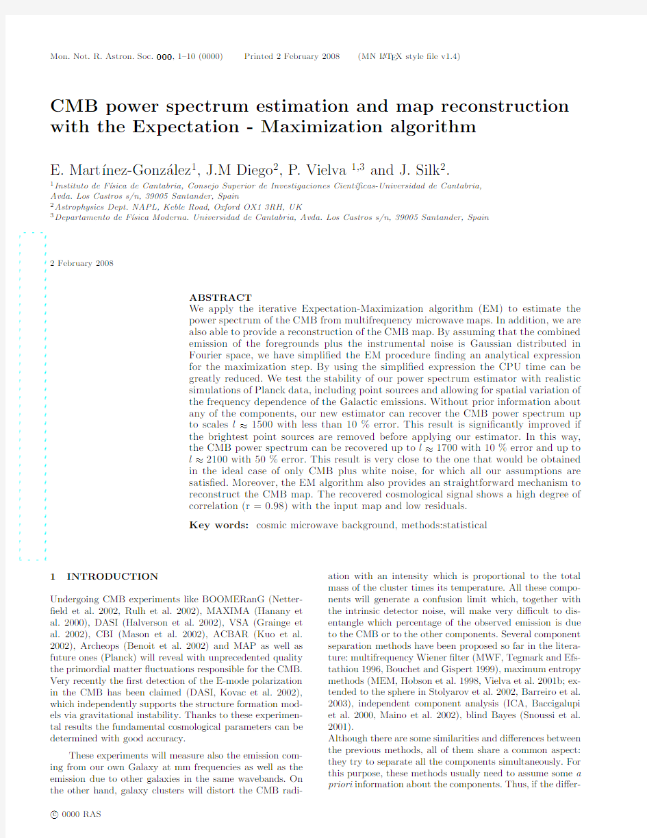
Figure1.Realistic simulations of the data,covering a12.8o×12.8o patch,expected from the10Planck channels.The RMS amplitude (at353GHz and in?T/T thermodinamic temperature units)is4.26×10?5for the CMB,5.16×10?6for the PS emission,3.93×10?6 for the SZ contribution,5.82×10?5for the thermal dust,3.23×10?7for the free-free radiation,1.46×10?6for the synchrotron emission and it is almost negligible in the case of the spinning dust(see text).

c 0000RAS,MNRAS000,1–10

CMB power spectrum with EM

7

x10

?11

Figure 2.Recovered power spectrum by our estimator.The solid line is the true power spectrum and the dotted and dashed lines represent the recovered power spectrum obtained by our estima-tor directly from the data and the one recovered after previous subtraction of the brightest point sources,respectively.P(k)is in ?T/T units.Notice that the multipole l is related to the wave number k through l ≈28k

.

Figure 3.Relative error in %of the recovered power spectrum by our estimator (dash-dotted line).For comparison we have plotted the errors obtained by our estimator in the ideal situation when only CMB and instrumental white noise are present in the data (see text).

sian ?uctuations.We would like to remark that synchrotron,thermal dust and the point source emissions have been sim-ulated using a frequency dependence which varies with the sky position.The simulated maps covering a patch of the sky of 12.8o ×12.8o ,as seen by the 10Planck channels,are shown in ?gure 1.4.2

A simple choice for the correlation matrix

In order to estimate the power spectrum of the CMB through eqn.(25)we still have to iterate a relatively com-plex expression containing a cocient of polynomials of order twice the number of channels and involving many terms.To further simplify the convergence of that equation we

will

Figure 4.Relative error in %of the recovered power spectrum by our estimator after the brightest point sources have been removed in all the channels (dash-dotted line).For comparison in the solid line we have plotted the errors obtained by our estimator in the ideal situation when only CMB and instrumental white noise are present in the data (see text).

only consider the diagonal terms of the covariance matrix,

making zero the other non-diagonal elements.This assump-tion does not take into account the correlations among the residuals at di?erent channels due to the Galactic compo-nents and compact sources.The former are re?ected at the low k -modes and their e?ect can be reduced by performing a simple Galactic subtraction as the one proposed by Diego et al.(2002).The later have their impact at intermediate (e.g.radio sources observed in the lowest resolution chan-nels)and large k -modes (e.g.infrared sources).However,as it will be shown below,once the brightest point sources are subtracted from the maps,the contribution of the remanent point sources is low enough to make their e?ect signi?cantly smaller.

In ?gure 2we present our results for the 10Planck chan-nels using the data obtained from the combination of the simulated components as described above (?gure 1).The comparison of the recovered spectrum with the true one shows a good agreement until k values larger than the one corresponding to the best antenna channels and the results start to be dominated by the deconvolved noise.

In order to better appreciate the di?erences,we show in ?gure 3the relative error,(P r (k )?P t (k ))/P t (k )%,where P r (k )is the estimator of equation 25.

In both large and relatively small scale range (small and relatively large k )our estimator ?nds a reasonably good estimation of the true power spectrum.The error is small (less than 10%)up to scales k ≈55(which corresponds to l ≈1500).The e?ect of only considering the diagonal terms of the residual covariance matrix is small (see also the comparison with the ideal case below).This fact proves the applicability of our assumption for the microwave data since our method is not very sensitive to the cross-correlations of the di?erent channels.

At very small scales (k >45or l >1300)the signal is below the noise level and the error bars grow quickly.Our estimator shows a clear bias toward higher values (we recover more power than the true one).This implies that

c

0000RAS,MNRAS 000,1–10

8 E.Mart′?nez-Gonz′a lez et al.

some of our assumptions are wrong at these small scales.The Gaussianity assumption is a good approximation in Fourier space at large k-modes(because of the dilution in many modes of the clear non-Gaussian features appearing in the real space).However,the uncorrelation assumption among frequency channels is a source of bias at these scales,since the bright point sources are strongly correlated.We have checked this point by removing the brightest point sources (but leaving the galaxy clusters and the weak point sources in the residual).We have used the Mexican Hat Wavelet (MHW)technique proposed by Vielva et al.(2001a)for re-moving point sources above the?uxes determined by the so-called50%error criterion used in that paper.These?uxes correspond to those detection limits above which the max-imum percentage of spurious detection is5%,being a de-tection spurious if the error in the amplitude estimation is larger than50%.After the subtraction,we applied our esti-mator to these new point-source-free maps.The?nal result is shown in?gure4.The e?ect of removing the brightest point sources is evident now.This result clearly shows how the bias can be corrected by removing the compact sources. The relative error does not change signi?cantly after remov-ing the point sources but the estimator is able to go up to scales k=60(l≈1700)with relative error<10%.The error is smaller than50%below k=75(l≈2100).

4.3Comparing with an ideal situation

It is interesting to answer whether or not the above results are close to the most optimistic case where all our assump-tions are right(Gaussianity and C diagonal).We will check this point in the simple(but unrealistic)case where our data consist only of CMB signal plus the corresponding instru-mental noise for each channel.In this simple case,our as-sumption of Gaussianity is right since both CMB and noise are Gaussian.The correlation matrix of the residual,C,will be exactly diagonal with the elements being the power spec-trum of the data minus the CMB power spectrum convolved with the antenna corresponding to each channel.

In?gures3and4we show the performance of the EM estimator in this ideal case(CMB plus noise)after combin-ing the10Planck channels.The result is surprisingly very similar to the one obtained in the realistic case where the brightest point sources have been subtracted(?gure4).This test shows how the EM estimator is extremely robust and can give results very close to the most optimal one.

4.4Map reconstruction

Using the expression given in equation22and the estimated power spectrum P r(k),we are able to recover the CMB map. As it was pointed out in Section3,due to the Gaussian-ity assumptions,equation22is nothing more than multifre-quency Wiener?lter(MWF).Hence,our map reconstruc-tion is a MWF focused on the CMB recovery.Let us re-mark that this approach di?ers from the traditional MWF already used in the microwave sky recovery(e.g.,Tegmark &Efstathiou1996,Bouchet&Gispert1999and Hobson et al1998).These works were focused on the all components separation,whereas our approach is devoted to reconstruct just the CMB signal.Even more,whereas the traditional approaches require previous knowledge of the power spec-tra(not only the CMB one,but also the power spectra of the foregrounds),the CMB power spectrum is a result of the blind EM method.This and the non requirement of any prior knowledge about the frequency dependence of the com-ponents,are the strongest points of the blind methods.In ?gure5we present the CMB map reconstruction(left)to-gether with the input one(right).Both maps have been con-volved with the best Planck resolution(FWHM=5’).The correlation between the input and recovered CMB maps is very good r=0.98(?gure6),whereas the slope of the best straightline?t is0.97.The residual CMB is dominated by the Galactic dust emission,since it is the most important foreground at low k-modes.Hence,by performing a simple dust subtraction as the one proposed by Diego et al.(2002)–which basically consists in using the857GHz channels as a dust template to be subtracted from the others channels–a signi?cant improvement in the CMB map reconstruction is achieved,being the RMS of the residual map lower than 15%.

5CONCLUSION

We have presented an e?cient estimator(eqn.25)of the CMB power spectrum.Our estimator is based on the EM algorithm and does not make use of any prior information whatsoever about any of the components.This renders sat-isfactory results,since we are able to recover the power spec-trum up to l≈1500with less than10%error.This limit can be improved if we remove the brightest compact sources,for instance applying the MHW technique poposed by Vielva et al.(2001a).After point source removal the estimator can recover the power spectrum up to l≈1700with less than 10%error and up to l≈2100with less than50%error.

Our results are very close to the optimal case when all our assumptions are satis?ed(only CMB and instrumen-tal noise are included in the simulations),as can be seen in?gure4.There are several CMB power spectrum estima-tions in the literature,given for di?erent component separa-tion techniques,like Bayesian methods(MEM:Hobson et al. 1998and Stolyarov et al.2002;and MWF:Tegmark&Efs-tathiou1996and Bouchet&Gispert1999)and blind source separation algorithms(ICA and FastICA:Baccigalupi et al.2000and Maino et al.2002;and Multi-Detector Multi-Component analysis:Delabrouille et al.2002).This work provides a CMB power spectrum that is comparable to or even better than the previous ones,being more robust than those,since previous knowledge about the underlying com-ponents is not requiered(contrary to the Bayesian meth-ods)and simulations used in previous works are signi?cantly more idealised than the ones used in this work(e.g.,lack of spatial variation of the frequency dependence for sev-eral components;absence of some of the components,like point sources or some Galactic foregrounds).On the other hand,our simulations account for the previous limitations including all the major microwave emissions and allowing for spatial variation of the frequency dependence.Finally,our method is able to reconstruct the CMB map using the esti-mated power spectrum and the MWF given in equation22. Let us remark that the MWF is obtained when the Gaus-sianity hypothesis is assumed,whereas the EM algorithm

c 0000RAS,MNRAS000,1–10

CMB power spectrum with EM

9

Figure 5.Left:CMB map reconstruction by our method (equation 22)using the recovered power spectrum obtained after previous subtraction of the brightest point sources.Right:Input CMB map.Both maps have been convolved with a Gaussian beam of FWHM =5

’

Figure 6.Correlation between the input and recovered CMB maps.The best strightline ?t is also plotted.

provides a more general procedure for component separa-tion.That hypothesis will be explored in a future work by including more realistic distributions for the di?erent com-ponents.In addition,we are working on a jointly deter-mination of the cosmological signals (CMB,SZ and point sources)using the EM algorithm and a point source de-tection tool.Finally,an extension of this algorithm to the sphere is straightforward and will be studied soon.

ACKNOWLEDGEMENTS

We thank J.Delabrouille for a critical reading of a pre-vious version of the manuscript which resulted in a sub-stantial improvement.We thank L.To?olatti for provid-ing us with the point source simulation,and B.T.Draine and https://www.360docs.net/doc/1f11298835.html,zarian for providing us with the emissivity pre-dicted by their spinning dust model.We appreciate in-teresting discussions with J.L.Sanz,R.B.Barreiro,D.Herranz and V.Stolyarov.We thank the RTN of the EU project HPRN-CT-2000-00124for partial ?nantial sup-port.EMG and PV acknowledge partial ?nancial support from the Spanish MCYT projects ESP2001-4542-PE and ESP2002-04141-C03-01.This research has been supported by a Marie Curie Fellowship of the European Community programme Improving the Human Research Potential and Socio-Economic knowledge under contract number HPMF-CT-2000-00967.PV acknowledges support from a fellowship of Universidad de Cantabria.

REFERENCES

Baccigalupi,C.,Bedini,L.,Burigana,C.,De Zotti,G.,Farusi,

A.,Maino,D.,Maris,M.,Perrota,F.,Salerno,E.,To?olatti,L.,Tonazzini,A.,2000,MNRAS,318,769

Barreiro,R.B.,Hobson,M.P.,Banday,A.J.,Lasenby,A.N.,Stol-yarov,V.,Vielva,P.,G′o rski,K.M.,2003,MNRAS,submitted Benoit,A.et al.,2002,A&A in press,astro-ph/0210306

Bouchet,F.R.,Gispert,R.&Puget,J.L.,1996in Drew,E.,

ed.,Proc.AIP Conf.384,The mm/sub-mm foregorunds and future CMB space missions.AIP Press,New York,p.255Bouchet,F.R.&Gispert R.,1999,NewA,4,443Cay′o n,L.,Sanz,J.L.,Barreiro,R.B.,Mart ′?nez-Gonz′a lez,E.,

Vielva,P.,To?olatti,L.,Silk,J.,Diego,J.M.&Arg¨u eso,F.,2000,MNRAS,315,757.

Chiang,L.Y.,Jogensen,H.E.,Naselsky,I.P.,Naselsky,P.D.,

Novikov,I.D.&Christensen,P.R.,2002,MNRAS,335,1054Delabrouille J.,Cardoso J.F.,Patanchon G.2002MNRAS sub-mitted.Preprint astro-ph/0211504.

Dempster,A.P.,Laird,N.M.,Rubin,D.B.,1977,Journal of the

Royal Statistical Society B,39,1.Diego,J.M.,Mart ′?nez-Gonz′a lez,E.,Sanz,J.L.,Cay′o n,L.&

Silk,J.,2001,MNRAS,325,1533.

Draine,B.T.&Lazarian,A.,1998,ApJ,494,L19.

Finkbeiner,D.P.,Davis,M.&Schlegel,D.J.,1999,ApJ,524,

867

c

0000RAS,MNRAS 000,1–10

10 E.Mart′?nez-Gonz′a lez et al.

Finkbeiner,D.P.,Schlegel,D.J.,Frank,C.&Heiles,C.,2002,

ApJ,566,898

Gaustad,J.E.,McCullough,P.R.,Rosing,W.&Van Buren,D.,

2001,PASP,113,1326

Grainge,K.et al.,2002,MNRAS submitted,astro-ph/0212495

Halverson,W.,et al.,2002,ApJ,568,38

Hanany,S.,et al.2000,ApJ,545,L1

Herranz,D.,Gallegos,J.E.,Sanz,J.L.&Mart′?nez-Gonz′a lez,

E.,2002a,MNRAS,334,533

Herranz,D.,Sanz,J.L.,Barreiro,R.B.&Mart′?nez-Gonz′a lez,

E.,2002b,ApJ,580,610

Herranz,D.,Sanz,J.L.,Hobson,M.P.,Barreiro,R.B.,Diego,J.

M.,Mart′?nez-Gonz′a lez,E.&Lasenby,A.N.,2002c,MNRAS,

336,1057

Hobson M.P.,Jones A.W.,Lasenby A.N.,Bouchet F.R.,1998,

MNRAS,300,1.

Hobson,M.P.,&McLachlan, C.,2002,MNRAS,submitted,

astro-ph/0204457

Kovac,J.,Leitch,E.M.,Pryke,C.,Carlstrom,J.E.,Halverson,

N.W.&Holzapfel,W.L.,2002,astro-ph/0209478

Kogut,A.,1999,ASP Conf.Ser.181:Microwave Foregrounds,

p.91.

Kuo,C.L.et al.,2002,astro-ph/0212289

Maino,D.,Farusi,A.,Baccigalupi,C.,Perrotta,F.,Banday,A.

J.,Bendini,L.,Burigana,C.,De Zotti,G.,G′o rski,K.M.&

Salerno,E.,2002,MNRAS,334,1,53

Mason,B.S.et al.,2002,ApJ,submitted,astro-ph/0205384.

McLachlan,G.&Krishnan,T.,1997,The EM Algorithm and Ex-

tensions.Wiley series in Probability and Statistics

Netter?eld,C.B.,et al.,2002,ApJ,571,604

de Oliveira-Costa,A.,Kogut,A.,Devlin,M.J.,Netter?eld,C.

B.,Page,L.A.&Wollack,E.J.,1997,ApJL,482,L17.

Reynolds,R.J.&Ha?ner,L.M.,2000,ASP Conference Series,

IAU Symposium#201,in press

Rulh,J.E.el al.,2002,astro-ph/0212229

Sanz,J.L.,Herranz,D.&Mart′?nez-Gonz′a lez,E.,2001,ApJ,552,

484

Snoussi,H.,Patanchon,G.,Mac′?as-P′e rez,J.F.,Mohammad-

Djafari,A.&Delabrouille,J.,2002,Proceedings of the MAX-

ENT2001international workshop,vol.568,388

Seljak,U.&Zaldarriaga,M.,1996,ApJ,469,437.

Stolyarov,V.,Hobson M.P.,Ashdwon,M.A.J.&Lasenby A.

N.,2002,MNRAS,336,97

Tegmark,M.,Efstathiou,G.,1996,MNRAS,281,1297

Tegmark,M.,de Oliveira-Costa,A.,1998,MNRAS,500,83

To?olatti,L.,Arg¨u eso,F.,De Zoti,G.,Mazzei,P.,Franceschini,

A.,Danese,L.&Burigana,C.,1998,MNRAS,297,117.

Vielva P.,Mart′?nez-Gonz′a lez E.,Cay′o n L.,Diego J.M.,Sanz

J.L.,To?olatti L.,2001a,MNRAS,326,181.

Vielva P.,Barreiro R.B.,Hobson M.P.,Mart′?nez-Gonz′a lez E.,

Lasenby A.N.,Sanz J.L.,To?olatti L.,2001b,MNRAS ac-

cepted.astro-ph/0105387

This paper has been produced using the Royal Astronomical

Society/Blackwell Science L A T E X style?le.

c 0000RAS,MNRAS000,1–10