Face Alignment by Explicit Shape Regression

Int J Comput Vis

DOI10.1007/s11263-013-0667-3

Face Alignment by Explicit Shape Regression Xudong Cao·Yichen Wei·Fang Wen·Jian Sun

Received:28December2012/Accepted:7October2013

?Springer Science+Business Media New York2013

Abstract We present a very ef?cient,highly accurate,“Explicit Shape Regression”approach for face alignment. Unlike previous regression-based approaches,we directly learn a vectorial regression function to infer the whole facial shape(a set of facial landmarks)from the image and explic-itly minimize the alignment errors over the training data.The inherent shape constraint is naturally encoded into the regres-sor in a cascaded learning framework and applied from coarse to?ne during the test,without using a?xed parametric shape model as in most previous methods.To make the regression more effective and ef?cient,we design a two-level boosted regression,shape indexed features and a correlation-based feature selection method.This combination enables us to learn accurate models from large training data in a short time(20min for2,000training images),and run regres-sion extremely fast in test(15ms for a87landmarks shape). Experiments on challenging data show that our approach sig-ni?cantly outperforms the state-of-the-art in terms of both accuracy and ef?ciency.

Keywords Face alignment·Shape indexed feature·Correlation based feature selection·Non-parametric shape constraint·Tow-level boosted regression

X.Cao(B)·Y.Wei·F.Wen·J.Sun

Visual Computing Group,Microsoft Research Asia,Beijing, People’s Republic of China

e-mail:xudongca@https://www.360docs.net/doc/2711709638.html,

Y.Wei

e-mail:yichenw@https://www.360docs.net/doc/2711709638.html,

F.Wen

e-mail:fangwen@https://www.360docs.net/doc/2711709638.html,

J.Sun

e-mail:jiansun@https://www.360docs.net/doc/2711709638.html, 1Introduction

Face alignment or locating semantic facial landmarks such as eyes,nose,mouth and chin,is essential for tasks like face recognition,face tracking,face animation and3D face mod-eling.With the explosive increase in personal and web photos nowadays,a fully automatic,highly ef?cient and robust face alignment method is in demand.Such requirements are still challenging for current approaches in unconstrained environ-ments,due to large variations on facial appearance,illumi-nation,and partial occlusions.

A face shape S=[x1,y1,...,x N fp,y N fp]T consists of N fp facial landmarks.Given a face image,the goal of face align-ment is to estimate a shape S that is as close as possible to the true shape?S,i.e.,minimizing

||S??S||2.(1)

The alignment error in Eq.(1)is usually used to guide the training and evaluate the performance.However,during test-ing,we cannot directly minimize it as?S is unknown.Accord-ing to how S is estimated,most alignment approaches can be classi?ed into two categories:optimization-based and regression-based.

Optimization-based methods minimize another error function that is correlated to(1)instead.Such methods depend on the goodness of the error function and whether it can be optimized well.For example,the AAM approach (Matthews and Baker2004;Sauer and Cootes2011;Saragih and Goecke2007;Cootes et al.2001)reconstructs the entire face using an appearance model and estimates the shape by minimizing the texture residual.Because the learned appear-ance models have limited expressive power to capture com-plex and subtle face image variations in pose,expression,and illumination,it may not work well on unseen faces.It is also

Int J Comput Vis well known that AAM is sensitive to the initialization due to

the gradient descent optimization.

Regression-based methods learn a regression function that

directly maps image appearance to the target output.The

complex variations are learnt from large training data and

testing is usually ef?cient.However,previous such methods (Cristinacce and Cootes2007;Valstar et al.2010;Dollar et al.2010;Sauer and Cootes2011;Saragih and Goecke2007) have certain drawbacks in attaining the goal of minimizing Eq.(1).Approaches in(Dollar et al.2010;Sauer and Cootes 2011;Saragih and Goecke2007)rely on a parametric model (e.g.,AAM)and minimize model parameter errors in the training.This is indirect and sub-optimal because smaller parameter errors are not necessarily equivalent to smaller alignment errors.Approaches in(Cristinacce and Cootes 2007;Valstar et al.2010)learn regressors for individual land-marks,effectively using(1)as their loss functions.However, because only local image patches are used in training and appearance correlation between landmarks is not exploited, such learned regressors are usually weak and cannot handle large pose variation and partial occlusion.

We notice that the shape constraint is essential in all meth-ods.Only a few salient landmarks(e.g.,eye centers,mouth corners)can be reliably characterized by their image appear-ances.Many other non-salient landmarks(e.g.,points along face contour)need help from the shape constraint—the cor-relation between landmarks.Most previous works use a para-metric shape model to enforce such a constraint,such as PCA model in AAM(Cootes et al.2001;Matthews and Baker 2004)and ASM(Cootes et al.1995;Cristinacce and Cootes 2007).

Despite of the success of parametric shape models,the model?exibility(e.g.,PCA dimension)is often heuristically determined.Furthermore,using a?xed shape model in an iterative alignment process(as most methods do)may also be suboptimal.For example,in initial stages(the shape is far from the true target),it is favorable to use a restricted model for fast convergence and better regularization;in late stages (the shape has been roughly aligned),we may want to use a more?exible shape model with more subtle variations for re?nement.To our knowledge,adapting such shape model ?exibility is rarely exploited in the literature.

In this paper,we present a novel regression-based approach without using any parametric shape models.The regressor is trained by explicitly minimizing the alignment error over training data in a holistic manner—all facial land-marks are regressed jointly.The general idea of regressing non-parametric shape has also been explored by Zhou and Comaniciu(2007).

Our regressor realizes the shape constraint in an non-parametric manner:the regressed shape is always a lin-ear combination of all training shapes.Also,using fea-tures across the image for all landmarks is more discrimina-

(a

(c)(d)

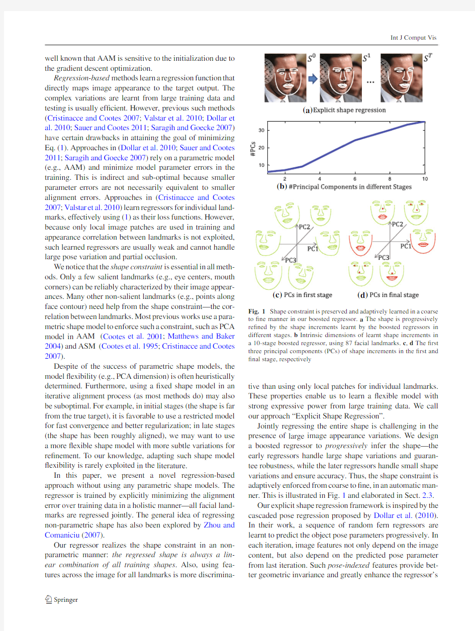
Fig.1Shape constraint is preserved and adaptively learned in a coarse to?ne manner in our boosted regressor.a The shape is progressively re?ned by the shape increments learnt by the boosted regressors in different stages.b Intrinsic dimensions of learnt shape increments in a10-stage boosted regressor,using87facial landmarks.c,d The?rst three principal components(PCs)of shape increments in the?rst and ?nal stage,respectively

tive than using only local patches for individual landmarks. These properties enable us to learn a?exible model with strong expressive power from large training data.We call our approach“Explicit Shape Regression”.

Jointly regressing the entire shape is challenging in the presence of large image appearance variations.We design a boosted regressor to progressively infer the shape—the early regressors handle large shape variations and guaran-tee robustness,while the later regressors handle small shape variations and ensure accuracy.Thus,the shape constraint is adaptively enforced from coarse to?ne,in an automatic man-ner.This is illustrated in Fig.1and elaborated in Sect.2.3.

Our explicit shape regression framework is inspired by the cascaded pose regression proposed by Dollar et al.(2010). In their work,a sequence of random fern regressors are learnt to predict the object pose parameters progressively.In each iteration,image features not only depend on the image content,but also depend on the predicted pose parameter from last iteration.Such pose-indexed features provide bet-ter geometric invariance and greatly enhance the regressor’s

Int J Comput Vis

performance.In their experiment,this method has also been

used to estimate face shape which is modeled by a simple

parametric ellipse(Dollar et al.2010).

Our method improves the cascaded pose regression frame-

work in several important aspects and works better for face

alignment problem.We adopt a non-parametric representa-

tion,directly estimate the facial landmarks by minimizing

the alignment error instead of parameter error.Consequently,

the underlying shape constraint is preserved automatically.

To address the very challenging high-dimensional regres-

sion problem,we further propose several improvements:a

two-level boosted regression,effective shape indexed fea-

tures,a fast correlation-based feature selection method and

sparse coding based model compression so that:(1)we can

quickly learn accurate models from large training data(20

min on2,000training samples);(2)the resulting regressor is

extremely ef?cient in the test(15ms for87facial landmarks);

(3)the model size is reasonably small(a few megabytes)and

applicable in many scenarios.We show superior results on

several challenging datasets.

2Face Alignment by Shape Regression

2.1The Shape Regression Framework

In this section,we describe our shape regression framework

and discuss how it?t to the face alignment task.

We cast our solution to shape regression task into the gra-

dient boosting regression(Friedman2001;Duffy and Helm-

bold2002)framework,which is a representative approach of

ensemble learning.In training,it sequentially learns a series

of weak learners to greedily minimize the regression loss

function.In testing,it simply combine the pre-learnt weak

learners in an additive manner to give the?nal prediction.

Before specifying how to resolve face alignment task in

gradient boosting framework,we?rst clarify a simple and

basic term,i.e.the normalized shape.Provided the prede?ned

mean shapeˉS,the normalized shape of an input shape S is obtained by a similarity transform which aligns the input

shape to the mean shape1to minimizes their L2distance, M S=argmin

M

||ˉS?M?S||2,(2)

where M S?S is the normalized shape.Now we are ready to describe our shape regression framework.

In training,given N training samples{I i,?S i,S0i}N i=1, the stage regressors(R1,...,R T)are sequentially learnt to

1It is also interesting to know that the mean shape is de?ned as the average of the normalized training shapes.Although it sounds like a circular de?nition,we still can compute the mean shape in an iterative way.Readers are recommended to Active Shape Model(Cootes et al. 1995)method for details.reduce the alignment errors on training set.In stage each t, the stage regressor R t is formally learnt as follows,

R t=argmin

R

N

i=1

||y i?R(I i,S t?1

i

)||2(3)

y i=M S t?1

i

?(?S i?S t?1

i

),

where S t?1

i

is the estimated shape in previous stage t?1,

M

S t?1

i

?(?S i?S t?1

i

)is the normalized regression target which will be discussed later.Please note herein we only apply the scale and rotation transformation to normalize the regression target.

In testing,given a facial image I and an initial shape S0, the stage regressor computes a normalized shape increment from image features and then updates the face shape,in a cascaded manner:

S t i=S t?1

i

+M?1

S t?1

i

?R t(I i,S t?1

i

),(4) where the stage regressor R t updates the previous shape S t?1to the new shape S t in stage t.Note we only scale and rotate(without translating)the output of the stage regression according to the angle and the scale of the previous shape.

2.1.1Discussion

Although our basic face alignment framework follows gradi-ent boosting framework,there are three components speci?-cally designed for the shape regression tasks.As these com-ponents are generic,regardless of the speci?c forms of the weak learner and the feature used for learning,it is worth clarifying and discussing them here.

Shape Indexed Feature The feature for learning the weak learner R t depends on both image I and previous estimated shape S t?1.It improves the performance by achieving geo-metric invariance.In other words,the feature is extracted relative to S t?1to eliminate two kinds of variations:the vari-ations due to scale,rotation and translation and the variations due to identity,pose and expression(i.e.the similarity trans-form M?1

S t?1

and the normalized shape M S t?1?S t?1).It is worth mentioning that although shape indexed feature sounds more complex,our designed feature is extremely cheap to be computed and does not require image warping.The details of our feature will be described in Sect.2.4.

Regressing the Normalized Target Instead of learning the

mapping from shape indexed feature to?S i?S t?1

i

,we argue the regression task will be simpli?ed if we regress the normal-

ized target M

S t?1

i

?(?S i?S t?1

i

).Because the normalized tar-get is invariant to similarity transform.To better understand its advantage,imagine two identical facial images with the estimated shape.One of them is changed by similarity trans-form while the other is kept unchanged.Due to the transform, the regression target(shape increments)of the transformed

Int J Comput Vis image are different from that of the unchanged one.Hence

the regression task is complicated.In contrast,the regression

task will keep simple if we regress the normalized targets,

which are still the same for both samples.

Data Augmentation and Multiple Initialization Unlike

typical regression task,the sample of our shape regression

task is a triple which is de?ned by the facial image,the

groundtruth shape and the initial shape i.e.{I i,?S i,S0i}.So

we can augment the samples by generating multiple initial

shapes for one image.In fact,it turns out such simple oper-

ation not only effectively improves generalization of train-

ing,but also reduces the variation of the?nal prediction by

bagging the results obtained by multiple initializations.See

Sect.3for experimental validations and further discussions.

To make the training and testing our framework clear,we

format them in the pseudo codes style.

Algorithm1Explicit Shape Regression(ESR)

Variables:Training images and labeled shapes{I l,?S l}L l=1;ESR model

{R t}T t=1;Testing image I;Predicted shape S;TrainParams{times of

data augment N aug,number of stages T};

TestParams{number of multiple initializations N int};

InitSet which contains exemplar shapes for initialization

ESRTraining({I l,?S l}L l=1,TrainParams,InitSet)

//augment training data

{I i,?S i,S0i}N i=1←Initialization({I l,?S l}L l=1,N aug,InitSet)

for t from1to T

Y←{M

S t?1

i ?(?S i?S t?1

i

)}N i=1//compute normalized targets

R t←LearnStageRegressor(Y,{I i,S t?1

i }N i=1)//using Eq.(3)

for i from1to N

S t i←S t?1

i +M?1

S t?1

i

?R t(I i,S t?1

i

)

return{R t}T t=1

ESRTesting(I,{R t}T t=1,TestParams,InitSet)

//multiple initializations

{I i,?,S0i}N int i=1←Initialization({I,?},N int,InitSet) for t from1to T

for i from1to N int

S t i←S t?1

i +M?1

S t?1

i

?R t(I i,S t?1

i

)

S←CombineMultipleResutls({S T i}N int i=1)

return S

Initialization({I c,?S c}C c=1,D,InitSet)

i←1

for c from1to C

for d from1to D

S o i←sampling an exemplar shape from InitSet

{I o i,?S o i}←{I c,?S c}

i←i+1

return{I o i,?S o i,S o i}C D i=1

The details about combining multiple results and initial-ization(including constructing InitSet and sampling from InitSet)will be discussed later in Sect.3.

As the stage regressor plays a vital role in our shape regres-sion framework,we will focus on it next.We will discuss what kinds of regressors are suitable for our framework and present a series of methods for effectively learning the stage regressor.

2.2Two-Level Boosted Regression

Conventionally,the stage regressor R t,is a quite weak regres-sor such as a decision stump(Cristinacce and Cootes 2007)or a fern(Dollar et al.2010).However,in our early experiments,we found that such regressors result in slow convergence in training and poor performance in the testing.

We conjecture this is due to two reasons:?rst,regressing the entire shape(as large as dozens of landmarks)is too dif?-cult to be handled by a weak regressor in each stage;second, the shape indexed feature will be unreliable if the previous regressors are too weak to provide fairly reliable shape esti-mation,so will the regressor based on the shape indexed feature.Therefore it is crucial to learn a strong regressor that can rapidly reduce the alignment error of all training samples in each stage.

Generally speaking,any kinds of regressors with strong ?tting capacity will be desirable.In our case,we again inves-tigate boosted regression as the stage regressor R t.Therefore threre are two-levels boosted regression in our method,i.e. the basic face alignment framework(external-level)and the stage regressor R t(internal-level).To avoid terminology con-fusion,we term the weak learner of the internal-level boosted regression,as primitive regressor.

It is worth mentioning that other strong regressors have also been investigated by two notable works.Sun et al. (2013)investigated the regressor based on convolutional neural network.Xiong and De la Torre(2013)investi-gated the linear regression with strong hand-craft feature i.e. SIFT.

Although the external-and internal-level boosted regres-sion bear some similarities,there is a key differences.The difference is that the shape indexed image features are?xed in the internal-level,i.e.,they are indexed only relative to the previous estimated shape S t?1and no longer change when those primitive regressor are being learnt.2This is impor-tant,as each primitive regressor is rather weak,allowing fea-ture indexing will frequently change the features,leading to unstable consequences.Also the?xed features can lead to much faster training,as will be described later.In our exper-iments,we found using two-level boosted regression is more accurate than one level under the same training effort,e.g., T=10,K=500is better than one level of T=5,000,as shown in Table4.

2Otherwise this degenerates to a one level boosted regression.

Int J Comput Vis

2.3Primitive Regressor

We use a fern as our primitive regressor.The fern was ?rstly introduced for classi?cation by Ozuysal et al.(2010)and later used for regression by Dollar et al.(2010).

A fern is a composition of F (5in our implementation)features and thresholds that divide the feature space and all training samples into 2F bins.Each bin b is associated with a regression output y b .Learning a fern involves a simple task and a hard task.The simple task refers to learning the outputs in bins.The hard task refers to learning the structure (the features and the splitting thresholds).We will handle the simple task ?rst,and resolve the hard task in the Sect.2.5later.

Let the targets of all training samples be {?y i }N i =1.The pre-diction/output of a bin should minimize its mean square dis-tance from the targets for all training samples falling into this bin.

y b =argmin

y

i ∈Ωb

||?y i ?y ||2,(5)where the set Ωb indicates the samples in the b th bin.It is easy to see that the optimal solution is the average over all targets in this bin.

y b =

i ∈Ωb ?y i |Ωb |.(6)To overcome over-?tting in the case of insuf?cient training data in the bin,a shrinkage is performed (Friedman 2001;Ozuysal et al.2010)as

y b =11+β/|Ωb |

i ∈Ωb ?y

i |Ωb |,(7)

where βis a free shrinkage parameter.When the bin has suf?cient training samples,βmakes little effect;otherwise,it adaptively reduces the magnitude of the estimation.2.3.1Non-parametric Shape Constraint

By directly regressing the entire shape and explicitly mini-mizing the shape alignment error in Eq.(1),the correlation between the shape coordinates is preserved.Because each shape update is additive as in Eqs.(4),(6)and (7),it can be shown that the ?nal regressed shape S is the sum of initial shape S 0and the linear combination of all training shapes:S =S 0

+

N i =1

w i ?S

i .(8)

Therefore,as long as the initial shape S 0satis?es the

shape constraint,the regressed shape is always constrained to reside in the linear subspace constructed by all train-ing shapes .In fact,any intermediate shape in the regression

also satis?es the https://www.360docs.net/doc/2711709638.html,pare to the pre-?xed PCA

shape model,the non-parametric shape constraint is adap-tively determined during the learning.

To illustrate the adaptive shape constraint,we perform PCA on all the shape increments stored in K ferns (2F ×K in total)in each stage t .As shown in Fig.1,the intrinsic dimension (by retaining 95%energy)of such shape spaces increases during the learning.Therefore,the shape constraint is automatically encoded in the regressors in a coarse to ?ne manner .Figure 1also shows the ?rst three principal com-ponents of the learnt shape increments (plus a mean shape)in ?rst and ?nal stage.As shown in Fig.1c,d,the shape updates learned by the ?rst stage regressor are dominated by global rough shape changes such as yaw,roll and scaling.In contrast,the shape updates of the ?nal stage regressor are dominated by the subtle variations such as face contour,and motions in the mouth,nose and eyes.2.4Shape Indexed (Image)Features

For ef?cient regression,we use simple pixel-difference features,i.e.,the intensity difference of two pixels in the image.Such features are extremely cheap to compute and powerful enough given suf?cient training data (Ozuysal et al.2010;Shotton et al.2011;Dollar et al.2010).

To let the pixel-difference achieve geometric invariance,we need to make the extracted raw pixel invariant to two kinds of variations:the variations due to similarity transform (scale,rotation and translation)and the variations due to the normalized shape (3D-poses,expressions and identities).In this work,we propose to index a pixel by the esti-mated shape.Speci?cally,we index a pixel by the local coordinate l =( x l , y l )with respect to a landmark in the normalized face.The superscript l indicates which land-mark this pixel is relative to.As Fig.2shows,such index-ing holds invariance against the variations mentioned above and make the algorithm robust.In addition,it also enable us sampling more useful candidate features distributed around salient landmarks (e.g.,a good pixel difference feature could be “eye center is darker than nose tip”or “two eye centers are similar”).

(a )(b)

Fig.2Pixels indexed by the same local coordinates have the same semantic meaning (a ),but pixels indexed by the same global coordinates have different semantic meanings due to the face shape variation (b )

Int J Comput Vis

In practical implementation,unlike previous works (Cristinacce and Cootes2007;Valstar et al.2010;Sauer and Cootes2011)which requires image warping,we instead transform the local coordinate back to the global coordinates on the original image to extract the shape indexed pixels and then compute the pixel-difference features.This leads to much faster testing speed.

Let the estimated shape of a sample be S.The location of the m th landmark is obtained byπl?S,where the operatorπl gets the x and y coordinates of m th landmark from the shape vector.Provided the local coordinate l,the corresponding global coordinates on the original image can formally repre-sented as follows.3

πl?S+M?1S? l(9) Note that although the l is identical for different samples, the global coordinates for extracting raw pixels are adaptively adjusted for different samples to ensure geometric invariance. Herein we only scale and rotate(without translating)the local coordinates according to the angle and the scale of the shape.

For each stage regressor R t in the external-level,we ran-domly generate P local coordinates{ lαα}Pα=1which de?ne P shape indexed pixels.Each local coordinate is generated by?rst randomly selecting a landmark(e.g.lαth landmark) and then draw random x-and y-offset from uniform distri-bution.The P pixels result in P2pixel-difference features. Now,the new challenge is how to quickly select effective features from such a large pool.

2.5Correlation-Based Feature Selection

To form a good fern regressor,F out of P2features are https://www.360docs.net/doc/2711709638.html,ually,this is done by randomly generating a pool of ferns and selecting the one with minimum regression error as in(5)(Ozuysal et al.2010;Dollar et al.2010).We denote this method as best-of-n,where n is the size of the pool.Due to the combinatorial explosion,it is unfeasible to evaluate(5) for all of the compositional features.As illustrated in Table5, the error is only slightly reduced by increasing n from1to 1024,but the training time is signi?cantly longer.

To better explore the huge feature space in a short time and generate good candidate ferns,we exploit the correlation between features and the regression target.We expect that a good fern should satisfy two properties:(1)each feature in the fern should be highly correlated to the regression target;

(2)correlation between features should be low so they are complementary when composed.

To?nd features satisfying such properties,we propose a correlation-based feature selection method.Let Y be the

3According to aforementioned de?nition,the global coordinates are computed via M?1S?(πl?M?1S?S+ l).By simplifying this formula, we get Eq.(9)Algorithm2Shape indexed features

Variables:images and corresponding estimated shapes{I i,S i}N i=1; number of shape indexed pixel features P;number of facial points N fp; the range of local coordinateκ;local coordinates{ lαα}Pα=1;

shape indexed pixel featuresρ∈ N×P;

shape indexed pixel-difference features X∈ N×P2; GenerateShapeIndexedFeatures({I i,S i}N i=1,N fp,P,κ)

{ lαα}Pα=1←GenerateLocalCoordinates(FeatureParams)

ρ←ExtractShapeIndexedPixels({I i,S i}N i=1,{ lαα}Pα=1)

X←pairwise difference of all columns ofρ

return{ lαα}Pα=1,ρ,X

GenerateLocalCoordinates(N fp,P,κ)

forαfrom1to P

lα←randomly drawn a integer in[1,N fp]

lαα←randomly drawn two?oats in[?κ,κ]

return{ lαα}Pα=1

ExtractShapeIndexedPixels({I i,S i}N i=1,{ lαα}Pα=1)

for i from1to N

forαfrom1to P

μα←πlα?S i+M?1S

i

? lα

ρiα←I i(μα)

returnρ

regression target with N(the number of samples)rows and 2N fp columns.Let X be pixel-difference features matrix with N rows and P2columns.Each column X j of the feature matrix represents a pixel-difference feature.We want to select F columns of X which are highly correlated with Y.Since Y is a matrix,we use a projection v,which is a column vector drawn from unit Gaussian,to project Y into a column vector Y prob=Y v.The feature which maximizes its correlation (Pearson Correlation)with the projected target is selected. j opt=argmin

j

corr(Y prob,X j)(10)

By repeating this procedure F times,with different random projections,we obtain F desirable features.

The random projection serves two purposes:it can pre-serve proximity(Bingham and Mannila2001)such that the features correlated to the projection are also discriminative to delta shape;the multiple projections have low correlations with a high probability and the selected features are likely to be complementary.As shown in Table5,the proposed corre-lation based method can select good features in a short time and is much better than the best-of-n method.

2.6Fast Correlation Computation

At?rst glance,we need to compute the correlation for all can-didate features to select a feature.The complexity is linear to the number of training samples and the number of pixel-difference features,i.e.O(N P2).As the size of feature pool scales square to the number of sampled pixels,the computa-

Int J Comput Vis

tion will be very expensive,even with moderate number of pixels (e.g.400pixels leads to 160,000candidate features!).Fortunately the computational complexity can be reduced from O (N P 2)to O (N P )by the following facts:The cor-relation between the regression target and a pixel-difference feature (ρm ?ρn )can be represented as follows.corr (Y proj ,ρm ?ρn )=

cov (Y proj ,ρm )?cov (Y proj ,ρn )

σ(Y proj )σ(ρm ?ρn )

σ(ρm ?ρn )=cov (ρm ,ρm )

+cov (ρn ,ρn )?2cov (ρm ,ρn )

(11)

We can see that the correlation is composed by two cat-egories of covariances:the target-pixel covariance and the pixel–pixel covariance.The target-pixel covariance refers to the covariance between the projected target and pixel fea-ture,e.g.,cov (Y proj ,ρm )and cov (Y proj ,ρn ).The pixel–pixel covariance refers to the covariance among different pixel fea-tures,e.g.,cov (ρm ,ρm ),cov (ρn ,ρn )and cov (ρm ,ρn ).As the shape indexed pixels are ?xed in the internal-level boosted regression,the pixel–pixel covariances can be pre-computed and reused within each internal-level boosted regression.For each primitive regressor,we only need to compute all target-pixel covariances to compose the correlations,which scales linear to the number of pixel features.Therefore the com-plexity is reduced from O (N P 2)to O (N P ).Algorithm 3Correlation-based feature selection

Input :regression targets Y ∈ N ×2N fp ;shape indexed pixel features ρ∈ N ×P ;pixel-pixel covariance cov (ρ)∈ P ×P ;number of features of a fern F ;

Output :The selected pixel-difference features {ρm f ?ρn f }F f =1and the

corresponding indices {m f ,n f }F f =1;

CorrelationBasedFeatureSelection (Y ,cov (ρ),F )

for f from 1to F

v ←randn (2N fp ,1)//draw a random projection from unit Gaussian Y prob ←Y v //random projection

cov (Y prob ,ρ)∈ 1×P ←compute target-pixel covariance σ(Y prob )←compute sample variance of Y prob m f =1;n f =1;for m from 1to P for n from 1to P

corr (Y prob ,ρm ?ρn )←compute correlation using Eq.(11)if corr (Y prob ,ρm ?ρn )>corr (Y prob ,ρm f ?ρn f )m f =m ;n f =n ;

return {ρm f ?ρn f }F f =1,{m f ,n f }F f =1

2.7Internal-Level Boosted Regression

As aforementioned,at each stage t ,we need to learn to a stage regressor to predict the normalized shape increments from the shape indexed features.Since strong ?tting capacity is vital to the ?nal performance,we again exploit the boosted regression to form the stage regressor.To distinguish it from

the external-level shape regression framework,we term it as

internal-level boosted regression.With the prepared ingredi-ents in previous three sections,we are ready to describe how to learn the internal-level boosted regression.

The internal-boosted regression consists of K primitive regressors {r 1,...,r K },which are in fact ferns.In testing,we combine them in an additive manner to predict the output.In training,the primitive regressors are sequentially learnt to greedily ?t the regression targets,in other words,each primi-tive regressor handles the residues left by previous regressors.In each iteration,the residues are used as the new targets for learning a new primitive regressor.The learning procedure are essentially identical for all primitive regressors,which can be describe as follows.

–Features Selecting F pixel-difference features using cor-relation based feature selection method.

–Thresholds Randomly sampling F i.i.d.thresholds from an uniform distribution.4

–Outputs Partitioning all training samples into different bins using the learnt features and thresholds.Then,learn-ing the outputs of the bins using Eq.(7).

Algorithm 4Internal-level boosted regression

Variables :regression targets Y ∈ N ×2N fp ;training images and corresponding estimated shapes {I i ,S i }N i =1;training parameters TrainParams {N fp ,P ,κ,F ,K };the stage regressor R ;testing image and corresponding estimated shape {I ,S };

LearnStageRegressor (Y ,{I i ,S i }N i =1,TrainParams ){ l αα}P

α=1←GenerateLocalCoordinates (N fp ,P ,κ)

ρ←ExtractShapeIndexedPixels ({I i ,S i }N i =1,{ l αα}P

α=1)cov (ρ)←pre-compute pixel-pixel covariance Y 0←Y //initialization for k from 1to K

{ρm f ?ρn f }F f =1,{m f ,n f }F f =1←

CorrelationBasedFeatureSelection (Y k ?1,cov (ρ),F ){θf }F f =1←sample F thresholds from an uniform distribution {Ωb }2F b =1←partition training samples into 2F bins {y b }2F

b =1←compute the outputs of all bins using Eq.(7)

r k ←{{m f ,n f }F f =1,{θf }F f =1,{y b }2F

b =1}//construct a fern Y k ←Y k ?1?r k ({ρm f ?ρn f }F f =1)//update the targets

R ←{{r k }K k =1,{ l αα}P α=1}//construct stage regressor

return R

ApplyStageRegressor (I ,S ,R )//i.e.R (I ,S )

ρ←ExtractShapeIndexedPixels ({I ,S },{ l αα}P α=1)

δS ←0

for k from 1to K

δS ←δS +r k ({ρm f ?ρn f }F f =1)return δS

4

Provided the range of pixel difference feature is [?c ,c ],the range of the uniform distribution is [?0.2c ,0.2c ].

Int J Comput Vis 2.8Model Compression

By memorizing the?tting procedures in the regression

model,our method gains very ef?cient testing speed.How-

ever,comparing with optimization based approaches,our

regression based method leads higher storage cost.The stored

delta shapes in the ferns’leaves contributes to the main

cost in the total storage,which can be quantitatively com-

puted via8N fp T K2F,where T K2F gives the number of all

leaves of T K random ferns in T stages,8N fp is the stor-

age of a delta shape in a single leaf.For example,provided

T=10,K=500,F=5and N fp=194,the storage is

around240mb,which is unaffordable in many real scenarios

such as mobile phones and embedded devices.

A straight forward way to compress model size is via

principal component analysis(Jolliffe2005).However,since

PCA only exploits orthogonal undercompleted basis in cod-

ing,its compression capability is limited.To further com-

press the model size,we adopt sparse coding which not only

takes the advantage of overcompleted basis but also enforces

sparse regularization in its objective.

Formally,the objective of sparse coding in a certain leave

of fern can be expressed as follows:

min x

i∈Ωb

?y i?Bx 22,s.t. x 0≤Q,(12)

where the?y i is the regression target;B is the basis for sparse coding;Q the is the upper bound of the number of non-zero codes(Q=5in our implementation).

The learning procedure of our model compression method consists of two steps in each stage.In the?rst step,the basis B of this stage is constructed.To learn the basis,we?rst run the non-sparse version of our method to obtain K ferns of this stage as well as the outputs stored in their leaves.Then the basis is constructed by random sampling5from the outputs in the leaves.

In the second step,we use the same method in Sect.2.5 to learn the structure of a fern.For each leaf,sparse codes are computed by optimizing the objective in Eq.(12)using the orthogonal matching pursuit method(Tropp and Gilbert 2007).Comparing with the shape increment,sparse codes require much less storage in leaves,especially when the dimension of the shape is high.

In testing,for K ferns in one stage,their non-zero codes in the leaves which are visited by the testing sample are lin-early summed up to form the?nal coef?cient x,then the output is computed via Bx,which contributes to the main computation.It is worth noting although the training of the 5We use random sampling for basis construction due to its simplicity and effectiveness.We also tried more sophisticated K-SVD method (Elad and Aharon2006)for learning basis.It yields similar performance comparing with random https://www.360docs.net/doc/2711709638.html,pressed version is more time-consuming,the testing is still as ef?cient as the original version.

3Implementation Details

We discuss more implementation details,including the shape initialization in training and testing,parameter setting and running performance.

3.1Initialization

As aforementioned,we generate a initial shape by sampling from an InitSet which contains exemplar shapes.The exem-plar shapes could be representative shapes selected from the training data,or the groundtruth shapes of the training data {?S i}N i=1.In training,we choose the later as the InitSet.While, in testing,we use the?rst for its storage ef?ciency.For one image,we draw the initial shapes without replacement to avoid duplicated samples.The scale and translation of the sampled shape should be adjusted to ensure that the corre-sponding face rectangle is the same with the face rectangle of the input facial image.

3.2Training Data Augmentation

Each training sample consists of a training image,an initial shape and a ground truth shape.To achieve better general-ization ability,we augment the training data by sampling multiple initializations(20in our implementation)for each training image.This is found to be very effective in obtain-ing robustness against large pose variation and rough initial shapes during the testing.

3.3Multiple Initializations in Testing

The regressor can give reasonable results with different initial shapes for a test image and the distribution of multiple results indicates the con?dence of estimation.As shown in Fig.3

, Fig.3Left results of5facial landmarks from multiple runs with differ-ent initial shapes.The distribution indicates the estimation con?dence: left eye and left mouth corner estimations are widely scattered and less stable,due to the local appearance noises.Right the average alignment error increases as the standard deviation of multiple results increases

Int J Comput Vis

Table1Training and testing times of our approach,measured on an Intel Core i72.93GHz CPU with C++implementation

Landmarks52987

Training(min)51021 Testing(ms)0.320.91 2.9

when multiple landmark estimations are tightly clustered, the result is accurate,and vice versa.In the test,we run the regressor several times(5in our implementation)and take the median result6as the?nal estimation.Each time the initial shape is randomly sampled from the training shapes.This further improves the accuracy.

3.4Running Time Performance

Table1summarizes the computational time of training(with 2,000training images)and testing for different number of landmarks.Our training is very ef?cient due to the fast fea-ture selection method.It takes minutes with40,000training samples(20initial shapes per image),The shape regression in the test is extremely ef?cient because most computation is pixel comparison,table look up and vector addition.It takes only15ms for predicting a shape with87landmarks(3ms ×5initializations).

3.5Parameter Settings

The number of features in a fern F and the shrinkage para-meterβadjust the trade off between?tting power in training and generalization ability in testing.They are set as F=5,β=1,000by cross validation.

Algorithm accuracy consistently increases as the number of stages in the two-level boosted regression(T,K)and num-ber of candidate features P2increases.Such parameters are empirically chosen as T=10,K=500,P=400for a good tradeoff between computational cost and accuracy.

The parameterκis used for generating the local coordi-nates relative to landmarks.We setκequal to0.3times of the distance between two pupils on the mean shape.

4Experiments

The experiments are performed in two parts.The?rst part compares our approach with previous works.The second part 6The median operation is performed on x and y coordinates of all landmarks individually.Although this may violate the shape constraint mentioned before,the resulting median shape is mostly correct as in most cases the multiple results are tightly clustered.We found such a simple median based fusion is comparable to more sophisticated strate-gies such as weighted combination of input shapes.validates the proposed approach and presents some interest-ing discussions.

We brie?y introduce the datasets used in the experiments. They present different challenges,due to different numbers of annotated landmarks and image variations.

BioID The dataset was proposed by Jesorsky et al.(2001) and widely used by previous methods.It consists of1,521 near frontal face images captured in a lab environment,and is therefore less challenging.We report our result on it for completeness.

LFPW The dataset was created by Belhumeur et al.(2011). Its full name is Labeled Face Parts in the Wild.The images are downloaded from internet and contain large variations in pose,illumination,expression and occlusion.It is intended to test the face alignment methods in unconstraint condi-tions.This dataset shares only web image URLs,but some URLs are no longer valid.We only downloaded812of the 1,100training images and249of the300test images.To acquire enough training data,we augment the training images to2,000in the same way as Belhumeur et al.(2011)did and use the available testing images.

LFW87The dataset was created by Liang et al.(2008).The images mainly come from the Labeled Face in the Wild (LFW)dataset(Huang et al.2008),which is acquired from uncontrolled conditions and is widely used in face recog-nition.In addition,it has87annotated landmarks,much more than that in BioID and LFPW,therefore,the perfor-mance of an algorithm relies more on its shape constraint. We use the same setting in Liang et al.(2008)’s work:the training set contains4,002images mainly from LFW,and the testing set contains1,716images which are all from LFW.

Helen The dataset was proposed by Le et al.(2012).It consists of2,330high resolution web images with194 annotated landmarks.The average size of face is550pix-els.Even the smallest face in the dataset is larger than 150pixels.It serves as a new benchmark which provides richer and more detailed information for accurate face alignment.

4.1Comparison with previous works

For comparisons,we use the alignment error in Eq.(1)as the evaluation metric.To make it invariant to face size,the error is not in pixels but normalized by the distance between the two pupils,similar to most previous works.

The following comparison shows that our approach out-performs the state of the art methods in both accuracy and ef?ciency,especially on the challenging LFPW and LFW87 datasets.Figures4,5,6and7show our results on challenging examples with large variations in pose,expression,illumina-tion and occlusion from the four datasets.

Int J Comput

Vis Fig.4Selected results from

LFPW

Fig.5Selected results from LFW87

4.1.1Comparison on LFPW

The consensus exemplar approach proposed by Belhumeur et al.(2011)is one of the state of the art methods.It was the best on BioID when published,and obtained good results on LFPW.

Comparison in Fig.8shows that most landmarks esti-mated by our approach are more than10%accurate7than 7The relative improvement is the ratio between the error reduction and the original error.

Int J Comput

Vis

Fig.6Selected results from

BioID

Fig.7Selected results from Helen dataset

Fig.8Results on the LFPW

circle radius is the average error

sents relative accuracy improvement

exemplars(CE)method proposed

accurate.Right top relative accuracy improvement of all landmarks over the results of CE method.Right bottom average error of all landmarks (Color?gure online)

the method proposed by Belhumeur et al.(2011)and our overall error is smaller.

In addition,our method is thousands of times faster.It takes around5ms per image(0.91×5initializations for29 landmarks).The method proposed by Belhumeur et al.(2011) uses expensive local landmark detectors(SIFT+SVM)and it takes more than10s8to run29detectors over the entire image.

on LFW87

(2008)proposed a component-based discrimina-

(CDS)method which trains a set of direction clas-

pre-de?ned facial components to guide the ASM

Their algorithm outperform previous ASM based works by a large margin.

the same root mean square error(RMSE)used in

et al.2008)as the evaluation metric.Table2

method is signi?cantly better.For the strict error

(5pixels),the error rate is reduced nearly by half, from25.3to13.9%.The superior performance on a large number of landmarks veri?es the effectiveness of proposed holistic shape regression and the encoded adaptive shape con-straint.

8Belhumeur et al.(2011)discussed in their work:“The localizer requires less than1s per?ducial on an Intel Core i73.06GHz machine”. We conjecture that it takes more than10s to locate29landmarks.

Int J Comput Vis

Table2Percentages of test images with root mean square error (RMSE)less than given thresholds on the LFW87dataset

RMSE<5Pixels<7.5Pixels<10Pixels

CDS(%)74.793.597.8

Our method(%)86.195.298.2

Bold values represent the best results under certain settings

Table3Comparison on Helen dataset

Method Mean Median Min Max

STASM0.1110.0940.0370.411 CompASM0.0910.0730.0350.402 Our method0.0570.0480.0240.16 The error of each sample is?rst individually computed by averaging the errors of194landmarks,and then the mean error across all testing samples is computed

Bold values represent the best results under certain settings

4.1.3Comparison on Helen

We adopt the same training and testing protocol as well as the same error metric used by Le et al.(2012).Speci?cally, we divide the Helen dataset into training set of2,000images and testing set of330images.As the pupils are not labeled in the Helen dataset,the distance between the centroids of two eyes are used to normalize the deviations from groundtruth.

We compare our method with STASM(Milborrow and Nicolls2008)and recently proposed CompASM(Le et al. 2012).As shown in Table3,our method outperforms them by a large https://www.360docs.net/doc/2711709638.html,paring with STASM and CompASM,our method reduces the mean error by50and40%respectively, meanwhile,the testing speed is even faster.

4.1.4Comparison to Previous Methods on BioID

Our model is trained on augmented LFPW training set and tested on the entire BioID dataset.

Figure9compares our method with previous methods (Vukadinovic and Pantic2005;Cristinacce and Cootes2006; Milborrow and Nicolls2008;Valstar et al.2010;Belhumeur et al.2011).Our result is the best but the improvement is mar-ginal.We believe this is because the performance on BioID is nearly maximized due to its simplicity.Note that our method is thousands of times faster than the second best method(Bel-humeur et al.2011).

4.2Algorithm Validation and Discussions

We verify the effectiveness of different components of the proposed approach.Such experiments are performed on the our augmented LFPW dataset.The dataset is split into two

Fig.9Cumulative error curves on the BioID dataset.For compari-son with previous results,only17landmarks are used(Cristinacce and Cootes2006).As our model is trained on LFPW images,for those land-marks with different de?nitions between the two datasets,a?xed offset is applied in the same way in Belhumeur et al.(2011)

Table4Tradeoffs between two levels boosted regression

Stage regressors(T)151******** Primitive regressors(K)50001000500501 Mean error(×10?2)15 6.2 3.3 4.5 5.2 Bold value represents the best results under certain settings

parts for training and testing.The training set contains1,500 images and the testing set contains500images.Parameters are?xed as in Sect.3,unless otherwise noted.

4.2.1Two-Level Boosted Regression

As discussed in Sect.2,the stage regressor exploits shape indexed features to obtain geometric invariance and decom-pose the original dif?cult problem into easier sub-tasks.The shape indexed features are?xed within the internal-level boosted regression to avoid instability.

Different tradeoffs between two-level boosted regression are presented in Table4,using the same number of ferns. On one extreme,regressing the whole shape in a single stage(T=1,K=5000)is clearly the worst.On the other extreme,using a single fern as the stage regressor (T=5000,K=1)also has poor generalization ability in the test.The optimal tradeoff(T=10,K=500)is found in between via cross validation.

4.2.2Shape Indexed Feature

We compare the global and local methods of shape indexed features.The mean error of local index method is0.033, which is much smaller than the mean error of global index method0.059.The superior accuracy supports the proposed local index method.

Int J Comput Vis

Table5Comparison between correlation based feature selection (CBFS)method and best-of-n feature selection methods

Best-of-n n=1n=32n=1024CBFS

Error(×10?2) 5.01 4.924.83 3.32 Time(s)0.1 3.0100.30.12 The training time is for one primitive regressor

Bold value represents the best results under certain

settings

Fig.10Average ranges of selected features in different stages.In stage 1,5and10,an exemplar feature(a pixel pair)is displayed on an image 4.2.3Feature Selection

The proposed correlation based feature selection method (CBFS)is compared with the commonly used best-of-n method(Ozuysal et al.2010;Dollar et al.2010)in Table5.CBFS can select good features rapidly and this is crucial to learn good models from large training data.

4.2.4Feature Range

The range of a feature is the distance between the pair of pixels normalized by the distance between the two pupils. Figure10shows the average ranges of selected features in the10stages.As observed,the selected features are adaptive to the different regression tasks.At?rst,long range features (e.g.,one pixel on the mouth and the other on the nose)are often selected for rough shape https://www.360docs.net/doc/2711709638.html,ter,short range features(e.g.,pixels around the eye center)are often selected for?ne tuning.

4.2.5Model Compression

We conduct experiments on both LFW87and Helen datasets to compare the sparse coding(SC)based compression method with PCA based compression method.

For sparse coding based method,the number of non-zero codes is5and the number of basis is512.For PCA based method,The principle components are computed by preserv-ing95%energy.Table6Model compression experiment

Dataset Raw PCA SC

Mean error(×10?2)LFW87 4.23 4.35 4.34 Model size(mb)LFW87118308 Comp.ratio LFW87–415 Mean error(×10?2)Helen194 5.70 5.83 5.79 Model size(mb)Helen1942404212 Comp.ratio Helen194–620 The suf?x of the name of the dataset means the number of annotated landmarks

As shown in Table6,the sparse coding based method outperforms the PCA based method both in the sense of compression ratio and accruacy.For example,on Helen dataset,the sparse coding based method archives20times compression.In contrast,the PCA based method achieves only6times compression at the cost of even lager mean error.

5Discussion and Conclusion

We have presented the explicit shape regression method for face alignment.By jointly regressing the entire shape and minimizing the alignment error,the shape constraint is auto-matically encoded.The resulting method is highly accurate, ef?cient,and can be used in real time applications such as face tracking.The explicit shape regression framework can also be applied to other problems like articulated object pose estimation and anatomic structure segmentation in medical images.

References

Belhumeur,P.,Jacobs,D.,Kriegman,D.,&Kumar,N.(2011).Local-izing parts of faces using a concensus of exemplars.In IEEE Con-ference on Computer Vision and Pattern Recognition(CVPR). Bingham,E.,&Mannila,H.(2001).Random projection in dimensional-ity reduction:Applications to image and text data.In ACM SIGKDD Conference on Knowledge Discovery and Data Mining(KDD). Cootes,T.,Edwards,G.,&Taylor,C.(2001).Active appearance models.

IEEE Transactions on Pattern Analysis and Machine Intelligence, 23(6),681–685.

Cootes,T.,Taylor,C.,Cooper,D.,Graham,J.,et al.(1995).Active shape models-their training and https://www.360docs.net/doc/2711709638.html,puter Vision and Image Understanding,61(1),38–59.

Cristinacce,D.,&Cootes,T.(2006).Feature detection and tracking with constrained local models.In British Machine Vision Conference (BMVC).

Cristinacce,D.,&Cootes,T.(2007).Boosted regression active shape models.In British Machine Vision Conference(BMVC).

Dollar,P.,Welinder,P.,&Perona,P.(2010).Cascaded pose regression.

In IEEE Conference on Computer Vision and Pattern Recognition (CVPR).

Int J Comput Vis

Duffy,N.,&Helmbold,D.P.(2002).Boosting methods for regression.

Machine Learning,47(2–3),153–200.

Elad,M.,&Aharon,M.(2006).Image denoising via sparse and redun-dant representations over learned dictionaries.IEEE Transactions on Image Processing,15(12),3736–3745.

Friedman,J.H.(2001).Greedy function approximation:A gradient boosting machine.The Annals of Statistics,29(5),1189–1232. Huang,G.,Mattar,M.,Berg,T.,Learned-Miller,E.et al.(2008)Labeled faces in the wild:A database forstudying face recognition in uncon-strained environments.In Workshop on Faces in’Real-Life’Images: Detection,Alignment,and Recognition.

Jesorsky,O.,Kirchberg,K.J.,&Frischholz,R.W.(2001).Robust face detection using the hausdorff distance(pp.90–95).New York: Springer.

Jolliffe,I.(2005).Principal component analysis.Wiley Online Library. Le,V.,Brandt,J.,Lin,Z.,Bourdev,L.,&Huang,T.(2012).Interactive facial feature localization.In European Conference on Computer Vision.

Liang,L.,Xiao,R.,Wen,F.,&Sun,J.(2008).Face alignment via component-based discriminative search.In European Conference on Computer Vision(ECCV).

Matthews,I.,&Baker,S.(2004).Active appearance models revisited.

International Journal of Computer Vision,60(2),135–164. Milborrow,S.,&Nicolls,F.(2008).Locating facial features with an extended active shape model.In European Conference on Computer Vision(ECCV).

Ozuysal,M.,Calonder,M.,Lepetit,V.,&Fua,P.(2010).Fast key-point recognition using random ferns.IEEE Transactions on Pattern Analysis and Machine Intelligence,32(3),448–461.Saragih,J.,&Goecke,R.(2007).A nonlinear discriminative approach to aam?tting.In International Conference on Computer Vision (ICCV).

Sauer,P.,&Cootes,C.T.T.(2011).Accurate regression procedures for active appearance models.In British Machine Vision Conference (BMVC).

Shotton,J.,Fitzgibbon,A.,Cook,M.,Sharp,T.,Finocchio,M.,Moore, R.,et al.(2011).Real-time human pose recognition in parts from single depth images.In IEEE Conference on Computer Vision and Pattern Recognition(CVPR).

Sun,Y.,Wang,X.,&Tang,X.(2013).Deep convolutional network cascade for facial point detection.In:IEEE Conference on Computer Vision and Pattern Recognition(CVPR).

Tropp,J.,&Gilbert,A.(2007).Signal recovery from random mea-surements via orthogonal matching pursuit.IEEE Transactions on Information Theory,53(12),4655–4666.

Valstar,M.,Martinez,B.,Binefa,X.,&Pantic,M.(2010).Facial point detection using boosted regression and graph models.In IEEE Con-ference on Computeer Vision and Pattern Recognition(CVPR). Vukadinovic,D.,&Pantic,M.(2005).Fully automatic facial feature point detection using gabor feature based boosted classi?ers.Interna-tional Conference on Systems,Man and Cybernetics,2,1692–1698. Xiong,X.,De la Torre,F.(2013)Supervised descent method and its applications to face alignment.In IEEE Conference on Computer Vision and Pattern Recognition(CVPR).

Zhou,S.K.,&Comaniciu,D.(2007).Shape regression machine.In Information Processing in Medical Imaging,(pp.13–25).Heidel-berg:Springer.