Battery Soc and SoH

Abstract—This paper describes experimental results aiming at analyzing lithium-ion batteries performances with aging, for different state of charge and temperatures. The results are provided from electrochemical impedance spectroscopy (EIS) measurements on new and aged cells. A climatic test chamber is used during experiments to simulate the conditions of the temperature. Experimental data are plotted over a broad spectrum of frequencies on Nyquist diagrams. We will also inspect the impact of the presence of a DC current during the EIS measurement. Finally, obtained results will be processed in a way to be used in a fuzzy logic system (FLS), to assess either the state of charge (SOC) or the state of health (SOH) of cells.

Index Terms—Lithium-ion batteries, Aging, EIS, State Of Charge, State Of Health, Fuzzy Logic System.

I.I NTRODUCTION

Lithium ion secondary batteries are now being used in wide applications especially for consumer electronics. However they are growing up in popularity for defense, automotive, and aerospace applications because they are light in weight, high in power, and long in cycle life.

Since several years SAFT has developed a range of lithium ion cells and batteries to cover the full spectrum of applications [1].

Ageing of lithium ion cells is an important question in all the applications that include this kind of batteries. It impacts on the battery performance [2], and hence, it modifies considerably the output parameters (such as the state of health).

For secondary batteries, the ageing includes both the calendar aging due to storage related to the time domain (in the range of months to years), and cycling aging related to the operation of charge/discharge of cells depending on the application profile.

To follow such a characteristic, electrochemical impedance spectroscopy (EIS) measurements on SAFT lithium ion batteries are carried out. EIS measurements interest both electrochemical and electrical researchers. The first ones, because it gives them information about kinetics in the * Corresponding author: Tel.: +33 5 57 10 94 18

E-mail address: ali.zenati@https://www.360docs.net/doc/6412796606.html, electrodes (such as Li+ diffusion rate) [3]. And the second ones, because it helps them to have an accurate equivalent circuit of the battery. This common measurement technique methodology has been studied for almost all battery chemistries not only for SOC, but also for SOH determination [4, 5].

Fuzzy logic system is one of the used methodologies, which combined with EIS measurement allows to assess the SOC and the SOH of batteries. Singh et al. have published noteworthy articles about using the EIS measurement with the fuzzy logic methodology to determine the SOC and/or the SOH of different battery chemistries from the VRLA batteries [6], to lithium-ion batteries used in defibrillators [7, 8], and other such as Nickel/metal hydride cells [9].

This paper shows experimental results obtained by EIS measurements on 2 types of Lithium-ion batteries, which had different aging processes and may differ at the electrochemical level, and their utilization as input parameters of a fuzzy logic system (FLS) to evaluate the SOC/SOH of batteries. Also, the word ‘battery’ will refer to either one cell or several cells.

II.O VERVIEW OF EXPERIMENT

https://www.360docs.net/doc/6412796606.html,ed lithium-ion cells

The cells used are lithium-ion SAFT power cells: VL30P which outputs a nominal capacity of 30 Ah and VL6P which outputs a nominal capacity of 6Ah. They have both a full charge voltage of 4V. And their chemistry is based on a natural graphite negative, a LiNi x Co y Al z O2 positive and 1M LiPF6 electrolyte. We will compare results obtained by each kind of cells.

For the VL30P, depicted in Figure 1, experimental tests were done for aged cells under different temperatures (0°C, 25°C/77°F and 45°C). This cells got accelerate ageing procedure during more than 6 months, in a climatic chamber at 60°C, in a fully state of charge. Accelerate ageing is caused by the application of a high temperature which contribute to degrade the age of batteries [10].

The climatic chamber can have a temperature fluctuating between -30°C and 60°C.

Estimation of the SOC and the SOH of Li-ion Batteries, by combining Impedance Measurements with the Fuzzy Logic Inference

A. Zenati1,*, Ph. Desprez1, and H. Razik2

1SAFT, 111-113, boulevard Alfred Daney, 33074 Bordeaux, France 2Université de Lyon, Lyon, F-69622, France; Université Lyon 1, Lyon, F-69622, France; CNRS, UMR5005, Laboratoire AMPERE, Villeurbanne, F-69622, France

Figure 1: Lithium-ion VL30P cell from SAFT

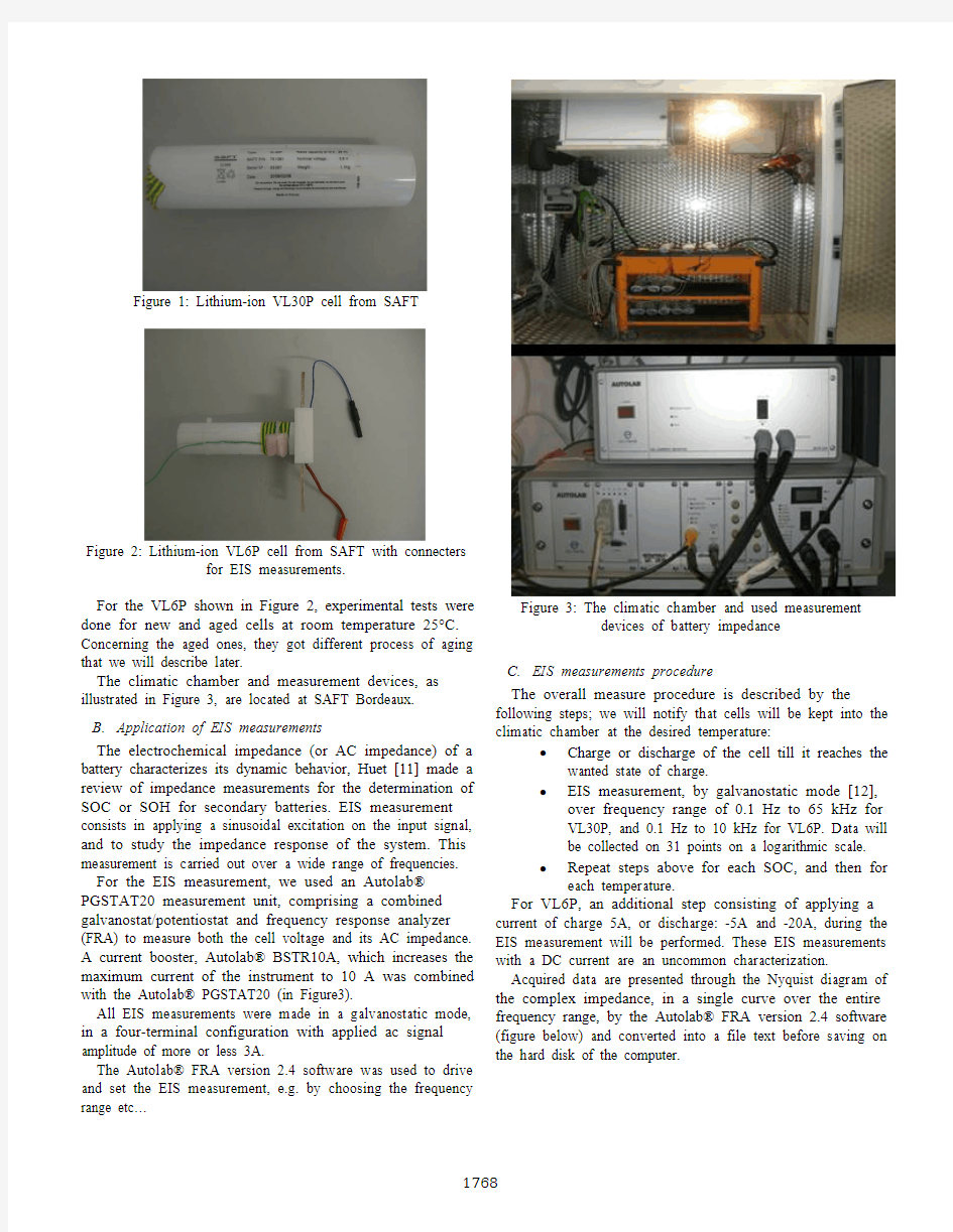
Figure 2: Lithium-ion VL6P cell from SAFT with connecters

for EIS measurements.

For the VL6P shown in Figure 2, experimental tests were done for new and aged cells at room temperature 25°C. Concerning the aged ones, they got different process of aging that we will describe later.

The climatic chamber and measurement devices, as illustrated in Figure 3, are located at SAFT Bordeaux.

B.Application of EIS measurements

The electrochemical impedance (or AC impedance) of a battery characterizes its dynamic behavior, Huet [11] made a review of impedance measurements for the determination of SOC or SOH for secondary batteries. EIS measurement consists in applying a sinusoidal excitation on the input signal, and to study the impedance response of the system. This measurement is carried out over a wide range of frequencies. For the EIS measurement, we used an Autolab? PGSTAT20 measurement unit, comprising a combined galvanostat/potentiostat and frequency response analyzer (FRA) to measure both the cell voltage and its AC impedance.

A current booster, Autolab? BSTR10A, which increases the maximum current of the instrument to 10 A was combined with the Autolab? PGSTAT20 (in Figure3).

All EIS measurements were made in a galvanostatic mode, in a four-terminal configuration with applied ac signal amplitude of more or less 3A.

The Autolab? FRA version 2.4 software was used to drive and set the EIS measurement, e.g. by choosing the frequency range etc…

Figure 3: The climatic chamber and used measurement

devices of battery impedance

C.EIS measurements procedure

The overall measure procedure is described by the following steps; we will notify that cells will be kept into the climatic chamber at the desired temperature:

?Charge or discharge of the cell till it reaches the wanted state of charge.

?EIS measurement, by galvanostatic mode [12], over frequency range of 0.1 Hz to 65 kHz for

VL30P, and 0.1 Hz to 10 kHz for VL6P. Data will

be collected on 31 points on a logarithmic scale.

?Repeat steps above for each SOC, and then for each temperature.

For VL6P, an additional step consisting of applying a current of charge 5A, or discharge: -5A and -20A, during the EIS measurement will be performed. These EIS measurements with a DC current are an uncommon characterization. Acquired data are presented through the Nyquist diagram of the complex impedance, in a single curve over the entire frequency range, by the Autolab? FRA version 2.4 software (figure below) and converted into a file text before saving on the hard disk of the computer.

Figure 4: Front panel of Autolab FRA software

D. Reminder on fuzzy logic principles

Fuzzy logic is a problem-solving methodology that provides a simple way to arrive at a definite conclusion based upon vague, ambiguous, imprecise, noisy, or missing input information. It is a branch of machine intelligence which includes multi-valued logic that helps computers which have statements that are true or false, to enable them to reason in a world where things are only partially true, just as the humans brain do.

The term "fuzzy logic" emerged as a consequence of the development of the theory of fuzzy sets proposed by Lotfi Zadeh, a professor at the University of California at Berkley, in 1965 [13], who established that the degree of truth (the value of a membership function) of a statement in fuzzy logic, can range between 0 and 1 and is not constrained to the two truth values {true (1), false (0)} as in classic binary logic [14].

We can resume the operating principle of a FLS, in a structure as simple as illustrated in the Figure 5 bellow with the following component, and thus decomposing in three well-marked steps:

Figure 5: Components of a fuzzy logic system

First step: Fuzzification:

Fuzzification is a mapping from the observed input to the fuzzy sets defined in the corresponding universe of discourse. In other words, it's called to the process of converting the crisp input into a fuzzy variable - using a fuzzy linguistic value - by

the mean of membership functions, to be used by reasoning mechanism.

Linguistic variables are the “vocabulary” of a FLS, or as defined, the fundamental knowledge representation unit in approximate reasoning [15]. Zadeh states: “By a linguistic variable we mean a variable whose values are words or sentences in a natural or artificial language”.

Based on this, each membership function of the universe of discourse of a variable, for example, can have a linguistic variable.

Generally to summarize, linguistic variables are non-numeric and often used to facilitate the expression of rules and facts.

The membership function is a generalisation of the indicator function in classical sets, which is defined by:

In FLS, it allows to represent the degree of truth of an input variable which belong totally (if the value is 1), partially (if the value is between 0 and 1), or not at all (if the value is 0) to the fuzzy set.

For the sake of simplicity, the most popular and typical shapes of membership functions include Triangular-, Trapezoidal-, Gaussian/bell-shaped functions. These three choices can be explained by the ease with which a parametric, functional description of the membership function can be obtained, stored with the minimal use of memory, and manipulated efficiently… Figure 6 depict the above choices

for the membership functions.

Figure 6: different shapes of membership functions

Second step: Rule base/ Data base:

The database involves the choice of membership functions for the input and output variables used in formulating the fuzzy rules, and also when required the choice of scaling factors.

The rule base describes the relationship between input and

output variables, this rules are all fired in parallel and are written in an ‘if…then’ linguistic format such as ‘if temperature is hot and discharge rate is high then output is low’.

The design parameters of the rule base include:

?Choice of process state and control output variables,

?Choice of the content of the rule-antecedent and the rule-consequent,

?Choice of term-sets for the process state and control output variables.

Second step: Inference Engine:

Mamdani's fuzzy inference method is the most commonly seen fuzzy methodology. Mamdani's method was among the first control systems built using fuzzy set theory. It was proposed in 1975 by Ebrahim Mamdani, who based his effort on Lotfi Zadeh's 1973 paper on fuzzy algorithms for complex systems and decision processes.

Its definition is based on the intersection operation, i.e.,

q

p

q

p∧

≡

→

.

The so-called Sugeno, or Takagi-Sugeno-Kang, method of fuzzy inference, introduced in 1985, is similar to the Mamdani method in many respects. The application of the fuzzy operator is exactly the same. The main difference between Mamdani and Sugeno is that the Sugeno output membership functions are either linear or constant.

A typical rule in a Sugeno fuzzy model has the form:

If Input 1 = x and Input 2 = y, then Output is z = ax + by + c For a zero-order Sugeno model, the output level z is a constant (a=b =0). This means that the output is a singleton rather than a fuzzy set, in the simplest Sugeno model.

Third step: Defuzzification:

Defuzzification converts the set of modified control output values into a single point-wise value which means that it transforms the fuzzy output sets to a crisp (real-valued) output. This step operates always with the output membership functions (which can be singletons), hence, we use specific methods to determinate the right value of the crisp output, such as:

?Center-of-Gravity/Area defuzzification,

?Center-of-Sums defuzzification,

?Center-of-Largest-Area defuzzification,

?First-of-Maxima defuzzification,

?Middle-of-Maxima defuzzification,

?Height defuzzification, …

The Center-of-Gravity method (also referred to as Center-of-Area method in the literature) is the best well-known and most utilized defuzzification method. It determines as its name indicates, the center of gravity below the combined output membership function.

The formula is given as follows:

For a membership function μU(u i), and U={u1,u2,…,u l}. Less used than the first method, the Middle-of-Maxima Defuzzification is instead used when we need to discriminate an output value, because it’s based on the calculus of the average’s outputs values the most likely.

III.R ESULTS AND DISCUSSION

A.EIS measurements on aged VL30P cells

As described in the measure procedure above, the aged VL30P cells will be in a steady state, i.e. no current DC (neither of charge nor discharge) will be applied during the EIS measurement. Representative results for each of the temperatures are shown below in function of three levels of the SOC: at 100%, 60% and 20%. Figures 5-a, 5-b and 5-c, illustrate EIS measurements for an aged VL30P for 0°C, 20°C, and 45°C respectively.

Figure 7-a: Results of EIS measurements at 0°C

Figure 7-b: Results of EIS measurements at 20°C

Figure 7-c: Results of EIS measurements at 45°C Figure 7-a shows that values of Z’o (defined as the point where Z’’ is equal to 0) at 20%, 60% and 100% of SOC almost overlap each other. However, Figure 7-b and Figure 7-c show that as the SOC decreases, the value of the resistance Z’o grows up.

This results show that for a temperature higher than 0°C, we can perform a fuzzy logic system to assess the value of the SOC. Inputs of the FLS will be based on previous data extracted from EIS measurements.

B.EIS measurements on aged VL6P cells

This time a current, either of charge or discharge, was applied during the EIS measurements, both on new and aged VL6P cells. As mentioned above, all measurements were conducted at room temperature, and the aged cells got different process of aging, hereafter the difference between cells:

?Cell 1, 2, 3 and 4: new VL6P cells. For these new cells, only analyses of EIS measurements of the

cell 1 are discussed here, because the other new

cells have the same features.

?Cell 5: aged cell, VL6P after 725 days of storage at 60°C, at 60% SOC.

?Cell 6: aged cell, VL6P after 500 days of storage at 60°C, at 60% SOC.

?Cell 7: aged cell, VL6P after 6200h of cycling according to a particular HEV accelerated profile. Analysis of the EIS measurement of the “Cell 1” at 80% of SOC, at room temperature 25°C, without applied DC current, under a current of charge of 5 A, and a current of discharge of both -5A and -20A, are gathered on the Nyquist diagram shown in Figure 8-a. Figure 8-b is a zoom of this Nyquist plot.

Figure 8-a: results of EIS measurement for VL6P Cell 1

Figure 8-b: zoom on the Nyquist plot of Figure 6-a

It appears that at Z”=0: as current DC decreases, the value of resistance Z’o does alike.

Figure 9-a, Figure 9-b and Figure 9-c display EIS measurement for the different cells at 80% of SOC, respectively without DC current, under a current of discharge of -5A and a current of charge of 5A.

From these experimental results, it emerges that not only does the value of Z’o rise up in aging cells, but it also changes depending of the type of ageing. In addition, we can observe that there is no difference between results obtained for EIS measurements with a current of charge or discharge, either for new or aged cells. Moreover, it is shown that having a current of charge/discharge during the EIS measurement has an influence on the AC impedance of lithium-ion batteries (see Figure 8-a, Figure 9-a, b, c).

Finally, fuzzy logic systems can be deducted from both results of EIS measurements without DC current and under a DC current of charge or discharge. And as we saw differences between impedance of new and aged cells, we can use EIS measurements to evaluate the SOH of cells, taking into account the used process of ageing, and the fact that we are either under DC current or not.

Figure 9-a: Results of EIS measurements on different VL6P

cells with no DC current

Figure 9-b: Results of EIS measurements on different VL6P cells with a DC current of discharge

Figure 9-c: Results of EIS measurements on different VL6P

cells with a DC current of charge

IV.C ONCLUSION

In this paper, we have presented EIS measurements for two types of lithium-ion cells, and how we can use obtained results to build a fuzzy logic system, by processing the correct input parameters. In addition to the chemical composition of cells, each condition of temperature and SOC has an impact on the use of batteries, specifically here on the AC impedance. Also the DC current during EIS measurement may have an influence on the AC impedance. The interpretation of results can differ depending on the expert’s knowledge either in electrochemical or electrical engineering.

Further studies are planned to be performed, showing how more extreme conditions of temperatures may impact on the cycle life of lithium-ion batteries, with more interest in other cell configurations.

R EFERENCES

[1]G. Sarre, Ph. Blanchard, M. Broussely, “Aging of lithium-ion batteries”,

Journal of Power Sources 127 (2004) 65–71.

[2] A. Jossen, “Fundamentals of battery dynamics”, Journal of Power

Sources 154 (2006) 530–538.

[3]M. Broussely, Ph. Biensan, F. Bonhomme, Ph. Blanchard, S. Herreyre,

K. Nechev, R.J. Staniewicz, “Main aging mechanisms in Li ion

batteries”, Journal of Power Sources 146 (2005) 90–96.

[4]S. Piller, M. Perrin, A. Jossen, “Methods dor state-of-charge

determination and their applications”, Journal of Power Sources 96

(2001) 113–120.

[5]S. Rodrigues, N. Munichandraiah, A. K. Shukla, “A review of state-of-

charge indication of batteries by means of a.c. impedance

measurements”, Journal of Power Sources 87 (2000) 12–20.

[6]P. Singh, S. Kaneria, J. Broadhead, X. Wang, J. Burdick, “Fuzzy logic

estimation of SOH of 125Ah VRLA batteries”, Telecommunications

Energy Conference, 2004. INTELEC 2004. 26th Annual International,

page(s): 524 – 531.

[7]P. Singh, R. Vinjamuri, X. Wang, D. Reisner, “Fuzzy logic modeling of

EIS measurements on lithium-ion batteries”, Electrochimica Acta 51

(2006) 1673–1679.

[8]P. Singh, R. Vinjamuri, X. Wang, D. Reisner, “Design and

implementation of a fuzzy logic-based state-of-charge meter for Li-ion

batteries used in portable defibrillators”, Journal of Power Sources 162

(2006) 829–836.

[9] A. J. Salkind, C. Fennie, P. Singh, T. Atwater, D. E. Reisner,

“Determination of state-of-charge and state-of-health of batteries by

fuzzy logic methodology”, Journal of Power Sources 80 (1999) 293-300.

[10]M. Broussely, S. Herreyre, Ph. Biensan, P. Kastztejna, K. Nechev, R.J.

Staniewicz, “Aging mechanism in Li-ion cells and calendar life

predictions”, Journal of Power Sources 97-98 (2001) 13–21.

[11] F. Huet, “A review of impedance measurements for determination of the

state-of-charge or state-of-health of secondary batteries”, Journal of

Power Sources 70 (1998) 59-69.

[12]P. Singh, C. Fennie Jr., D. Reisner, “Fuzzy logic modeling of SOC and

available capacity on nickel/metal hydride batteries”, Journal of Power

Sources 136 (2004) 322–333.

[13]Zadeh, L.A. (1965). "Fuzzy sets", Information and Control 8 (3): 338–

353.

[14]Novák, V., Perfilieva, I. and Mo?ko?, J. (1999) Mathematical principles

of fuzzy logic Dodrecht: Kluwer Academic. ISBN 0-7923-8595-0. [15]Zadeh, L.A., "The concept of a linguistic variable and its application to

approximate reasoning, Parts 1, 2, and 3," Information Sciences, 1975,

8:199-249, 8:301-357, 9:43-80.