An Interior Point Method Based on Nonlinear Complementarity Model for OPF Problems

An Interior Point Method Based on Nonlinear Complementarity Model for OPF Problems with Load Tap Changing Transformers

Bin LI

Depart. of Electrical

Engineering

Guangxi University Nanning,Guangxi, PR China lizhen@https://www.360docs.net/doc/6713026958.html,

Xiaoqing BAI

Depart. of Electrical

Engineering

Guangxi University

Nanning,Guangxi, PR China

baixq @https://www.360docs.net/doc/6713026958.html,

Hua WEI

Depart. of Electrical

Engineering

Guangxi University

Nanning,Guangxi, PR China

weihua @https://www.360docs.net/doc/6713026958.html,

Abstract: A nonlinear complementarity model for OPF problems with load tap changing transformers is created in this paper, and a modern interior point method for this model is presented as well. The proposed method includes two steps. Firstly, the OPF with the continuous variables is considering for obtaining the upper and lower bounds of the transformer taps. And then, the complementarity constraints of the transformer taps is modeled into OPF, which can be solved by the modern interior point method based on the results of the last step. Therefore, the discrete results of the LTC’s taps can be calculated accurately. This method can coordinate the illogicality between the calculating time and precision effectively. Extensive numerical simulations on IEEE test systems and the simulative power system with 232 and 1047 buses have shown that this method is efficient in solving OPF problem for the discrete variables. It possesses good convergence property within a very short time. Thus it is promising for the on-line applications.

Keywords: LTC transformers; discrete variable; complementarity model; optimal power flow

I INTRODUCTION

In recent years, Optimal Power Flow (OPF)[1] in power system has been developed greatly in terms of both the model expansion and the algorithm implementation, and its application has been extended increasingly. So far, OPF has become a necessary tool for network analysis and optimization in power system, and provides some fundamental data for other (power system application) PAS software.

In power systems, load tap changing transformers (LTCs) can be found at the power plants as step-up transformers, within the transmission system to control the reactive power flow and the voltage profile, and at substations feeding loading centers to keep the secondary voltage at an acceptable value when the primary voltage magnitudes undergo variations. Therefore, LTC tap is an important component in reactive power optimization and one of the important control variables in OPF.

The LTCs is a transformer with a variable tap ratio that can be used to control the voltage by one of its terminals. Since the variable tap ratios are discrete, OPF with LTC taps is a large scale of Mixed Integer Nonlinear Programming (MINP) with multi- constraints. However, there are still some problems to gain the precise solutions of LTC taps in OPF within the reasonable times. A brief review of recent methods for solving LTC taps in OPF is described as follows:

y Continuous rounding method. This is a de facto two-stage method used in engineering at present. In the first stage, LTC taps are considered as the continuous variables, and then the optimization results are rounded into integers.

Secondly, OPF problems with the rounded LTC taps as constants are calculated once again. Generally, suboptimal solutions are obtained by this method since LTC taps are not variables in the second stage.Furthermore, the solution errors may increase as the growth of system sizes and the number of discrete variables.

y Direct solution methods[2~4] such as cutting plane method, branch and bound method, and so on. Theoretically, these methods have the corresponding mathematical models and algorithms, with which the discrete LTC taps can be solved accurately. However, the computing consumption is very large, which is proportional to exponents of discrete variables. And the results are poor feasibility and taking extremely long period for solution.

y Artificial intelligence algorithms[5,6] such as simulated evolution programming method, simulated annealing method, and so on. These methods do not require the rigorous mathematic models, and can solve discrete LTC taps problems as well. However, the computing efficiency is unstable so that these methods are considered impractical.

y Alternative solution methods[7~8]. It is well known that the continuous LTC tap problems can be solved by IPM efficiently. But the discrete variables still can not be gained directly. On the other hand, although the artificial intelligence algorithms can achieve the discrete variables, the computing consumptions are very large. It’s a

978-1-4244-4813-5/10/$25.00 ?2010 IEEE

contradiction between time and precision during solution process. As a result, there are alternative solution methods, such as the combination of the continuous programming method and artificial intelligence algorithms. Basically, the continuous programming methods are used to solve the continuous variables and the artificial intelligence method are applied to the discrete variables. Two methods are adopted alternatively. However, the optimal solutions can not be guaranteed since the solution of the variables is accomplished in the different processes.

Currently, nonlinear programming problem with complementarity constraints [9,10] provides a new approach to solving MINP problems, whose key point is transforming the discrete problems into the complementarity constraints, and then solving by the modern interior-point algorithm. This paper presents an optimal power flow (OPF) based problems with incorporates complementarity constraints for load tap changing transformers (LTCs), and a modern interior point nonlinear programming algorithm as well. Extensive numerical simulations have shown that this method is efficient in solving OPF problem for the discrete variables. The paper is organized as follows: Section 2 presents a mathematical model for LTCs in OPF. The brief reviews of complementarity are described in Section 3. Section 4 shows the complementarity model and algorithm for LTCs. The numerical results and their discussion are presented in Section 5. Finally, conclusions are given in Section 6.

II

MATHEMATICAL MODEL FOR OPF

The OPF [11] problems with load tap changing transformers can be described as a mixed integer nonlinear programming problem.

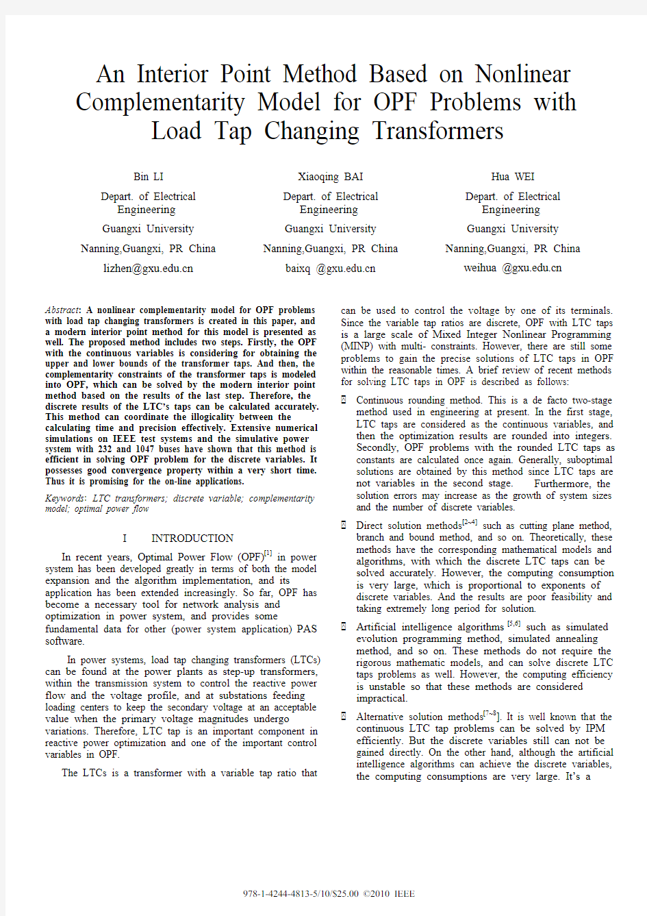
In this paper, the LTC transformer is modeled as a π equivalent circuit with elements that depend on the tap ratio. In Fig. 1, the LTC connected between nodes i and j has the variable tap ratio kij and the longitudinal admittance Yt. The admittance of the magnetizing branch has been neglected.

kij Yt

Fig. 1. The model of the LTC transformer

Without loss of generality, the objective functions are minimum active power loss or minimum reactive power loss of the following form in this study:

min ()G

DP

R

DQ

Gi Di i S i S Gi Di

i S i S P P f Q Q ∈∈∈∈????=????∑∑∑∑ （1） Where P Gi is the active power output at node i, P Di is the

active load at node i, Q Gi is the reactive power output at node i, Q Di is the reactive power load at node i, S G is the set of active generators, S R is the set of reactive power supplies, S DP is the set of active load, and S DQ is the set of reactive load. Subject to:

1) Equality constraints h(x):

y

Power flow equations for buses.

()1,1,222

1,1,1,2

cos cos cos cos cos 0sin sin sin K K

K

K K n n

Gi Di i it t it i im im m im

t t S m m S n i ii ii

i ij ij ij i ij ij j ij j j S n n Gi Di i it t it i ii im m im t t S m m S i ii i P P VY

V V k Y V V Y V k Y V k Y V Q Q VY V V k Y V V Y δδδαδδδδ′′=?=∈′=∈′′=≠=∈′???′′′′+?+=′???′′?∑∑∑∑∑()221,sin sin 0K n i i ij ij ij i ij ij j ij j j S V k Y V k Y V αδ′

=∈?

??

????????′′++=??

∑ (2)

Where n is the number of nodes in system; S N is the set of

system nodes; V i and δi are the voltage amplitude and the phase angle at node i ; Y ij and αij are the amplitude and the phase angle of transfer transadmittance between node i and j, and δij =δi –δj -αij . k ij is the LTC tap ratio between node i and j; S K is the set of the LTCs; S K ’ is the set of LTC at node i side, which containing ideal transformers; S K ”is the set of LTC at node j side, which excluding ideal transformers. y

Constraints for LTCs tap

()()()120

,ij

ij ij ij ij ijm K

k

k k k k k i j S ???=∈" （3）

Where k ij1k ij2…k ijm are the values corresponding to the LTCs

taps ratio, and m is the sum of the LTCs taps.

2) Inequality constraints g(x)

For different objective functions, the following constraints can be combined.

(,)Gi Gi Gi G Gi Gi Gi R Di Di Di DP Di Di Di DQ i i i N

ij ij ij L

P P P i S Q Q Q i S P P P i S Q Q Q i S V V V i S P P P i j S

?≤≤∈?

≤≤∈??≤≤∈??

≤≤∈??

≤≤∈??≤≤∈???"

（4） Where 2cos cos ij i ij ij i ij j ij

P V Y VY V αδ=?+ is the active power of the connection line between nodes i and j. S N is the set of lines

III NONLINEAR PROGRAMMING PROBLEM WITH

COMPLEMENTARITY CONSTRAINTS

In engineering and economical applications, the complementarity condition depicts the change of behavior of a system depending on the way certain conditions are satisfied.

The formulations of mathematical programs with complementarity constraints (MPCCs) is as follows [10,12~15]:

()()min. ().. ()0 () 00

f x s t h x

g g x g G x H x =≤≤≤⊥≥ (5)

(5) (5)(5)

a b c d

Where

n R ∈x , (): n R R → f x ,(): n m R R → h x ,

(): n r R R →g x ,():n p R R → G x ,():n p R R → H x . The complementarity condition (5d) stands for:

()0≥G x (6a ) ()0≥H x (6b )

()()0=i i G x H x (6c ) Eq. (6a~6c) holds only if one of the following situations is satisfied:

()()0,0i i G x H x =≥ (7a )

()()0,0i i G x H x ≥= (7b )

()()0,0==i i G x H x (7c ) The solutions (7a ) and (7b ) are said to satisfy strict complementarity conditions. The solution (7c ), in which both values are zero, exhibits non-strict complementarity behavior. Complementarity (7a ~7c ) represents a logical condition and must be expressed in analytic form if the MPCCs can be solved by using nonlinear programming methods. A popular reformulation of the MPCC is:

()()()()min. ()

.. ()0 () 0,0

f x s t h x

g g x g

G x H x G x H x =≤≤≥≥≤ (8)

(8)

(8)(8)(8)

a b c d e

This formulation preserves the solution set of the MPCCs but is not totally adequate because it violates the Mangasarian –Fromowitz constraint qualification (MFCQ) at any feasible point. This lack of regularity can create problems when applying classical nonlinear programming algorithms.I nterior methods exhibit inefficiencies caused by the conflicting goals of enforcing complementarity while keeping the variables x away from their bounds. Therefore, direct solution is difficult to achieve with conventional nonlinear planning algorithms including modern interior-point algorithm. Many studies have stimulated considerable interest in developing interior methods for MPCCs that guarantee both global convergence and efficient practical performance. The approaches can be broadly grouped into two categories [10,12,16]:

1). The first category comprises relaxation approaches,

where (8) is replaced by a family of problems in which (8e) is changed to:

()()i i G x H x εε?≤≤ （9） Where relaxation parameter 0ε> is introduced and

updated after each iteration, then decreases with ()()i i G x H x and approaches zero gradually. However, when ε becomes smaller, the numerical property will become

worse due to the shrunk solution domain.

Therefore, this method has certain requirement on the method for updating relaxation parameter ε. Presently there are two acceleration strategies in the process:

y

Acceleration of complementarity constraint factor

T w u p

ε= （10）

Where w is a complementarity constraint variable, u

is a relaxation factor, and p is the number of corresponding complementarity constraint variables.

y

Contraction of upper and lower limits of variable constraints

Integer variable is serialized during calculation. When it approaches its integer solution, the upper and the lower limits of constraints are contracted with adjacent integer solution as the center according to given policy, so that it approaches the integer solution in an accelerated manner.

2). The second category involves a regularization technique

based on an exact-penalty reformulation of the MPCCs. Here, (8e) is moved to the objective function in the form of a penalty term, so tha t (8a ) becomes:

()()()T

f x G x H x π+ (11)

Where 0π> is a penalty parameter. If π is chosen large

enough, the solution of the MPCCs can be recast as the minimization of a single penalty function. The appropriate value of π is, however, unknown in advance and must be estimated during the course of the minimization.

IV OPF COMPLEMENTARITY CONSTRAINTS

MODEL CONTAINING LTC TAPS

Generally, there are multiple ratios for LTC tap in power system. Eq. (3) is a polynomial expression with the number of ranks identical to that of LTC tap ratios. But this is not a nonlinear complementarity constraint condition. Therefore, it’s much more important to model the complementarity constraint condition for LTC taps for the algorithm implementation.

The strategy to model the complementarity constraint is obtaining the upper and lower bounds of the LTC taps by the modern interior point algorithm for the continuous OPF at first. The mathematical model can be simply expressed as below:

min.()..()0(),=≤≤≤≤∈

ij

ij ij K

f x s t h x

g g x g k k k i j S （12）

For the sake of space, the modern interior-point method is not described here. Please find the details in literatures [17-19].

If the optimal solution exists, then the continuous optimal

solutions for LTC tap can be obtained by the pre-calculation. However, the solutions are not always locating on the setting positions which are discrete values. Therefore, they are not feasible for the original model, but between two discrete positions [20], i.e., (1)ijn ij ij n k k k +≤≤, k ij =k ijn or k ij =k ij (n+1), where k ijn and k ij (n+1) are the two boundaries of LTC tap k ij . Thus, the complementarity constraint condition for LTC tap can be established as:

()()(1)0,+??=∈ij

ijn ij n ij K

k

k k k i j S （13）

Adding Eq. (13), the OPF based problem with

complementarity constraint models for discrete LTC taps can be modeled, and solved by modern interior-point method. The mathematical model can be simply expressed as:

()()(1)

(1)

min.()..()0()0

,++=≤≤≤≤??=∈ ijn ij ij n ij n ij ij ijn K

f x s t h x

g g x g k k k k

k k k i j S （14）

And then, for guarantying the convergence, relaxation

approaches is adopted for the complementarity constraint for LTC tap. So the above model is relaxed:

()()(1)

(1)min.()..()0(),ijn ij ij n ij n ij ij ijn K

f x s t h x

g g x g k k k k k k k i j S εε++=≤≤≤≤?≤??≤∈ （15）

where the acceleration strategy for ε selection is shrinking the

upper and the lower limits of the variables. In detail, a relatively large value can be taken for ε at the beginning, e.g., 0.1 with the algorithm’s convergence. And then εscales down proportionally depend on the decrease of complementarity interval in the modern interior-point algorithm.

V

NUMERICAL RESULTS AND DISCUSSION

The proposed algorithm for OPF with LTC taps has been coded in C and compiled on a Dell （2.8GHz ，2G ）/ PC. Six test systems are used to evaluate the performance of the algorithm.

Table 1 lists the features of the test systems. In the test cases, the objective function is minimized active power loss for the network and the convergence precision is 10-6.

Table 1. The structure of testing system

Name of system Number of buses Number of

lines P Gi Q Gi LTC

IEEE-14 14 20 5 5 3 IEEE-303043 6 64IEEE-118118186 15 549IEEE-300300409 21 69107SH-232232357 19 56143S-104710471182 68 152164

For simplicity, IEEE-30 is used to explain the

performance of the proposed algorithm. There are four LTCs in this system, and their adjustment ranges of ratio are all between 0.9 and 1.1, and the discrete positions are 0.9，0.92，0.94，0.96，0.98，1，1.02，1.04，1.06，1.08，and 1.1, respectively.

In optimization theory, the complementary gap is a very

important measure to judge the optimality of solutions and its change reflects the characteristic of the algorithm. When complementarity gap approaches zero, the solution trends to be optimal. On the other hand, its variation trend can reflect the characteristics of an algorithm. The faster the complementarity gap approaches zero monotonically, the better convergence performance the algorithm achieves. Fig. 2 shows the variation of complementarity gap during the test of IEEE-30 system. Both complementarity gaps converge into the setting precision range almost within identical iterations, and in terms of convergence speed, both of them can reduce to zero monotonically. The iterations of the complementarity model are more than that of the continuous model because the maximum amount of unbalance of complementarity constraint equation can’t converge within the same speed. But the complementarity model can finish within limited iterations. That is said, the proposed algorithm possesses satisfactory convergence and robustness property.

C o m p l e m e n t a r y g a p s

Iterations

Fig.2. Complementary gaps with iterations for IEEE-30 system

Fig. 3 depicts how the maximum mismatches of complementarity constraint equation for IEEE-30 system reduce with the iterations. Since the complementarity constraint equation has been transformed into inequation, its zero approximation depends on the strategy of ε selection. Therefore, the convergence speed of complementarity constraint is lower, but still can meet the precision requirement within limited iterations. That is, the discrete points are found under the precision requirement rather than approximate values.

-3

M a x i m u m m i s m a t c h o f c o m p l e m e n t a r i t y c o n s t r a i n t s e q u a t i o n

Iterations

Fig.3. Maximum mismatch of complementarity constraints equation with

iterations for IEEE-30 system

Fig.4 shows the optimal value of objective function on IEEE-30 system converge with iterations. The objective function is minimized active power loss. Their curves in Fig. 3 have slight difference which was caused by the discrete LTC taps. Therefore, OPF optimal solutions for the discrete LTC taps can be obtained by the algorithm .

Iterations

O b j e c t i v e f u n c t i o n

Fig.4. Objective function with iterations for IEEE-30 system

Table 2 shows the ratio values of four LTC taps in

IEEE-30 system. After convergence in the continuous pre-calculation, the LTC taps locate between two adjacent ratios. And then, the LTC taps will be one given accurate ratios after the complementarity model is converged. Obviously, they are the optimal solutions for the discrete variables. That is, the optimal solutions are obtained from the combination of all control variables and status variables, and should be the real optimal solutions instead of suboptimal solutions, which can be proved by the results in Table 3. Table 3 shows the difference of the tap ratios obtained from between the continuous rounding method and the proposed method. For example, the LTC tap of transformer 1 by the proposed method in IEEE-30 system is 1.079993, i.e., 1.08, while is 1.06 by continuous rounding method. Meanwhile, the value of the objective function based on complementarity model is 0.011992, while is 0.012009 by continuous rounding. It is obviously that the solution obtained by the continuous rounding method is not the optimal solution at all.

Table 2. Results of transformer tap for IEEE-30 system

transformer

pre-calculation

complementarity

model

continuous rounding method

1 1.064459 1.079993 1.06

2 0.906804 0.900000 0.90

3 0.98329

4 0.98000

5 0.984 0.970611 0.97999

6 0.98

Table 3. Comparison results for IEEE-30 system method

continuous calculation

continuous rounding

complemen tarity model

method

objective function 0.011955 0.012009 0.011992 iterations 13

26 48

computing time (ms)

0 0 31

Table 4 are the results of all test systems in this study, where k 1 is the iteration of pre-calculation, and k 2 is that of complementarity model; f 1 is the value of objective function of pre-calculation, and f 2 is that of complementarity model, where objective functions are both minimized active power loss, represented by per-unit value; T 1is the time used for convergence in pre-calculation, and T 2 is that of complementarity model. The computing times listed in IEEE-14 and IEEE-30 are zero, which means they are actually less than 16ms and only display as 0.

Table 4. Result of the test systems

system iterations objective function computing time (ms)

k 1k 2f 1 f 2 T 1T 2IEEE-1414340.089715 0.089723 00IEEE-3013350.011955 0.011992 00IEEE-11817480.720068 0.721315 47125IEEE-3001971 3.215196 3.221858 110405SH-23219580.552074 0.559891 78203S-1047

23

44

2.452004 2.461312 359701

Table 4 shows that pre-calculation with the continuous model for the boundaries of a transformer can benefit from the good convergence and rapid calculation of the modern interior-point algorithm. Furthermore, since the solution of the continuous model is used as the initial value, the ratios of LTC taps can be solved precisely with complementarity constraints. In the case of multiple transformer ratios, the computing efficiency is keeping high, and the iterations will not increase too much. As for the convergence speed, the proposed complementarity model is just several times faster than the continuous OPF model. The execution times increase rather linearly with the size of the system and the numbers of LTCs. Note that the typical CPU time of S-1047 is about several seconds which can fully meet the on-line requirement.

VI CONCLUSIONS

In this paper, an OPF complementarity constraint model with the discrete LTC taps is built, and a nonlinear complementarity constraint interior-point algorithm for solution is introduced. The characteristics of the method summarize as follows:

y By constructing the LTC taps into the complementarity constraints, the proposed method can coordinate the contradiction between the time consumptions and precisions within solving discrete variables with the conventional method. It can solve the discrete LTC taps in OPF precisely. y The solution of the model is optimal rather than suboptimal by combining the control and status variables together. y The fast convergence and rapid calculation of the proposed algorithm are guaranteed by using the modern IPM, which can meet the online requirement absolutely.

Extensive numerical simulations on IEEE test systems (IEEE-14~IEEE-300) and the simulative power systems (SH-232 and S-1047) have shown that the proposed method is promising for large scale OPF with the discrete LTC taps due

to its robustness and fast execution times. This method illustrates a good prospect of application and extension to solve the problems with discrete variable in the power system.

ACKNOWLEDGMENT

The project is supported by National Natural Science Foundation of China(NSFC)(50867001) 、by Guangxi Education Department under Grant GJK No. 200701MS145

and Specialized Research Fund for the Doctoral Program of Higher Education （20060593002）.

REFERENCES

[1].J. A. Momoh, R. J. Koessler and M. S. Bond, et al. Challenges to

optimal power flow. IEEE Trans. Power Syst, vol.12, no.1, pp.

444-455, 1997.

[2].X. Y. Ding, X. F. Wang and X. A. Zhang. Mixed integer optimal

power flow based on interior point cutting plane method. Proceedings

of the CSEE, vol.24, no.2, pp. 1-7, 2004.

[3].M.Delfanti, G.P.Granelli. Optimal capacitor placement using

deterministic and genetic algorithms. IEEE Trans. on Power Syst, vol.15, no.3, pp. 1041-1046, 2000.

[4].Y. Cheng, M. B. Liu. Reactive power optimization of large-scale

power systems with discrete control variables, Proceedings of the

CSEE, vol.21, no.5, pp. 54-60, 2002.

[5]. C. H. Liang, C. Y. Chung and K. P. Wong,Parallel Optimal Reactive

Power Flow Based on Cooperative Co-Evolutionary Differential

Evolution and Power System Decomposition. IEEE Trans. on Power

Syst, vol.22, no.1, pp. 249-257, 2007.

[6].M. Varadarajan, K.S. Swarup. Differential evolutionary algorithm for

optimal reactive power dispatch.Applied Soft Computing, vol.8, no.4,

pp. 205-215, 2008.

[7].W.Yan, F.Liu, and C.Y. Chung, A Hybrid Genetic Algorithm–Interior

Point Method for Optimal Reactive Power Flow.IEEE Trans. on

Power Syst, vol.21, no.3, pp. 1163-1169, 2006.

[8]. X.Y.Ding, X.F. Wang and H.Y. Chen. A combined algorithm for

optimal power flow. Proceedings of the CSEE, vol.22, no.12, pp.

11-16, 2002.

[9].W. Rosehart, C. Roman and A. Schellenberg. Optimal Power Flow

With Complementarity Constraints. IEEE Trans. on Power Syst,

vol.20, no.2, pp. 813-823, 2005.

[10].S. Leyffer, L.C.Gabriel and J.Nocedal. Interior Methods for

Mathematical Programs with Complementarity Constraints.SIAM

Journal on Optimization, vol.17, no.1, pp. 52–77, 2006.

[11].H. Wei, H. Sasaki and R. Yokoyama, et al. An interior point nonlinear

programming for optimal power flow problems with a novel data

structure.IEEE Trans. on Power Syst, vol.13, no.3, pp. 870-877, 1998. [12]. C. Roman, W. Rosehart. Complementarity model for generator buses

in opf-based maximum loading problems, IEEE Trans.on Power Syst.

vol.20, no.1, pp. 514–516, 2005.

[13]. C.Roman, W.Rosehart. Complementarity model for load tap changing

transformers in stability based OPF problem.Electric Power Systems

Research, vol.76, no.1, pp. 592–599, 2006.

[14].R.Fletcher, S.Leyffer. Numerical experience with solving MPECs as

NLPs. Optimization Methods and Software, vol. 19, no.1, pp. 15-40,

2004.

[15]. D.Ralph, S.J.Wright. Some properties of regularization and

penalization schemes for MPECs. Optimization Methods and Software.

vol. 19, no.5, pp. 527-556, 2004.

[16]. A. U. Raghunathan, L. T. Biegler. An Interior Point Method for

Mathematical Programs with Complementarity Constraints (MPCCs).

SIAM Journal on Optimization, vol. 15, no.3, pp. 720–750, 2005. [17]. A. Forsgren, P. E. Gill and M. H. Wright. Interior methods for

nonlinear optimization, SIAM Review, vol. 44, no.5, pp. 525-597, 2002. [18].H. Wei, H. Sasaki, J. Kubokawa, et al. A interior point nonlinear

programming for optimal power flow problems with a novel data

structure. IEEE Trans on Power Syst, vol. 13, no.3, pp. 870~877, 1998.

[19].H. Wei, H. Sasaki, J. Kubokawa, et al. Large Scale Hydro-Thermal

Optimal Power Flow Problems Based on Interior Point Nonlinear Programming. IEEE Trans on Power Syst, vol. 15, no.1, pp. 396-403, 2000.

[20]. A.D. Papalexopoulos, C.F. Imparato, F.F.Wu. Large-Scale Optimal

Power Flow: Effects of Initialization, Decoupling and Discretization.

IEEE Trans. on Power Systems, vol. 4, no.2, pp. 748～761, 1989.