intraprediction,HEVC里面的帧内编码详解

Intra Coding of the HEVC Standard

Jani Lainema,Frank Bossen,Member,IEEE,Woo-Jin Han,Member,IEEE,Junghye Min,and Kemal Ugur

Abstract—This paper provides an overview of the intra coding techniques in the High Ef?ciency Video Coding(HEVC)standard being developed by the Joint Collaborative Team on Video Coding (JCT-VC).The intra coding framework of HEVC follows that of traditional hybrid codecs and is built on spatial sample prediction followed by transform coding and postprocessing steps.Novel features contributing to the increased compression ef?ciency include a quadtree-based variable block size coding structure, block-size agnostic angular and planar prediction,adaptive pre-and post?ltering,and prediction direction-based transform coef?cient scanning.This paper discusses the design principles applied during the development of the new intra coding methods and analyzes the compression performance of the individual tools. Computational complexity of the introduced intra prediction algorithms is analyzed both by deriving operational cycle counts and benchmarking an optimized https://www.360docs.net/doc/871184343.html,ing objective metrics,the bitrate reduction provided by the HEVC intra coding over the H.264/advanced video coding reference is reported to be 22%on average and up to36%.Signi?cant subjective picture quality improvements are also reported when comparing the resulting pictures at?xed bitrate.

Index Terms—High Ef?ciency Video Coding(HEVC),image coding,intra prediction,Joint Collaborative Team on Video Coding(JCT-VC),video coding.

I.Introduction

T HE TWO prominent international organizations specify-ing video coding standards,namely ITU-T Video Coding Experts Group(VCEG)and ISO/IEC Moving Picture Experts Group(MPEG),formed the Joint Collaborative Team on Video Coding(JCT-VC)in April2010.Since then,JCT-VC has been working toward de?ning a next-generation video coding standard called High Ef?ciency Video Coding(HEVC).There are two major goals for this standard.First,it is targeted to achieve signi?cant improvements in coding ef?ciency com-pared to H.264/Advanced Video Coding(A VC)[1],especially when operating on high-resolution video content.Second,the standard should have low enough complexity to enable high-resolution high-quality video applications in various use cases, Manuscript received April13,2012;revised July18,2012;accepted August 21,2012.Date of publication October2,2012;date of current version January 8,2013.This work was supported by Gachon University under the Research Fund of2012GCU-2011-R288.This paper was recommended by Associate Editor O.C.Au.(Corresponding author:W.-J.Han.)

https://www.360docs.net/doc/871184343.html,inema and K.Ugur are with the Nokia Research Center,Tampere 33720,Finland(e-mail:https://www.360docs.net/doc/871184343.html,inema@https://www.360docs.net/doc/871184343.html,;kemal.ugur@https://www.360docs.net/doc/871184343.html,).

F.Bossen is with DOCOMO Innovations,Inc.,Palo Alto,CA94304USA (e-mail:bossen@https://www.360docs.net/doc/871184343.html,).

W.-J.Han is with Gachon University,Seongnam461-701,Korea(e-mail: hurumi@https://www.360docs.net/doc/871184343.html,).

J.Min is with Samsung Electronics,Suwon442-742,Korea(e-mail: jh643.min@https://www.360docs.net/doc/871184343.html,).

Color versions of one or more of the?gures in this paper are available online at https://www.360docs.net/doc/871184343.html,.

Digital Object Identi?er10.1109/TCSVT.2012.2221525including operation in mobile environments with tablets and mobile phones.

This paper analyzes different aspects of the HEVC intra coding process and discusses the motivation leading to the selected design.The analysis includes assessing coding ef?ciency of the individual tools contributing to the overall performance as well as studying complexity of the introduced new algorithms in detail.This paper also describes the methods HEVC utilizes to indicate the selected intra coding modes and further explains how the tools are integrated with the HEVC coding block architecture.

Intra coding in HEVC can be considered as an extension of H.264/A VC,as both approaches are based on spatial sample prediction followed by transform coding.The basic elements in the HEVC intra coding design include:

1)quadtree-based coding structure following the HEVC

block coding architecture;

2)angular prediction with33prediction directions;

3)planar prediction to generate smooth sample surfaces;

4)adaptive smoothing of the reference samples;

5)?ltering of the prediction block boundary samples;

6)prediction mode-dependent residual transform and coef-

?cient scanning;

7)intra mode coding based on contextual information.

In addition,the HEVC intra coding process shares several processing steps with HEVC inter coding.This processing, including,e.g.,transformation,quantization,entropy coding, reduction of blocking effects,and applying sample adaptive offsets(SAO),is outside of the scope of this paper.

This paper is organized as follows.Section II explains the motivation leading to the selected design for HEVC intra coding.It also describes the overall HEVC coding architecture and the new intra prediction tools introduced in the HEVC standard.Section III presents the intra mode coding and the residual coding approaches of the standard.Section IV provides complexity analysis of the introduced intra prediction processes with detailed information about the contribution of different intra prediction modes.Section V summarizes the compression ef?ciency gains provided by the proposed design and Section VI concludes this paper.

II.HEVC Intra Coding Architecture

In H.264/A VC,intra coding is based on spatial extrapolation of samples from previously decoded image blocks,followed by discrete cosine transform(DCT)-based transform coding [2].HEVC utilizes the same principle,but further extends it to be able to ef?ciently represent wider range of textural and

1051-8215/$31.00c 2012IEEE

structural information in images.The following aspects were considered during the course of HEVC project leading to the selected intra coding design.

1)Range of supported coding block sizes:H.264/A VC

supports intra coded blocks up to the size of16×16 pixels.This represents a very small area in a high-de?nition picture and is not large enough to ef?ciently represent certain textures.

2)Prediction of directional structures:H.264/A VC sup-

ports up to eight directional intra prediction modes for

a given block.This number is not adequate to predict

accurately directional structures present in typical video and image content,especially when larger block sizes are used.

3)Prediction of homogeneous regions:The plane mode of

H.264/A VC was designed to code homogeneous image

regions.However,this mode does not guarantee con-tinuity at block boundaries,which can create visible artifacts.Thus,a mode that guarantees continuous pre-diction sample surfaces would be desired.

4)Consistency across block sizes:H.264/A VC uses differ-

ent methods to predict a block depending on the size of the block and the color component the block represents.

A more consistent design is preferred,especially as

HEVC supports a large variety of block sizes.

5)Transforms for intra coding:H.264/A VC utilizes a?xed

DCT transform for a given block size.This design does not take into consideration different statistics of the pre-diction error along the horizontal and vertical directions depending on the directionality of the prediction.

6)Intra mode coding:Due to the substantially increased

number of intra modes,more ef?cient coding techniques are required for mode coding.

The coding structure utilized for intra coding in HEVC follows closely the overall architecture of the codec.Images are split into segments called coding units(CU),predic-tion units(PU),and transform units(TU).CU represent quadtree split regions that are used to separate the intra and inter coded blocks.Inside a CU,multiple nonoverlapping PU can be de?ned,each of which speci?es a region with individual prediction parameters.CU are further split into a quadtree of transform units,each TU having a possibility of applying residual coding with a transform of the size of the TU.

HEVC contains several elements improving the ef?ciency of intra prediction over earlier solutions.The introduced methods can model accurately different directional structures as well as smooth regions with gradually changing sample values. There is also emphasis on avoiding introduction of arti?cial edges with potential blocking effects.This is achieved by adaptive smoothing of the reference samples and smoothing the generated prediction boundary samples for DC and directly horizontal and vertical modes.

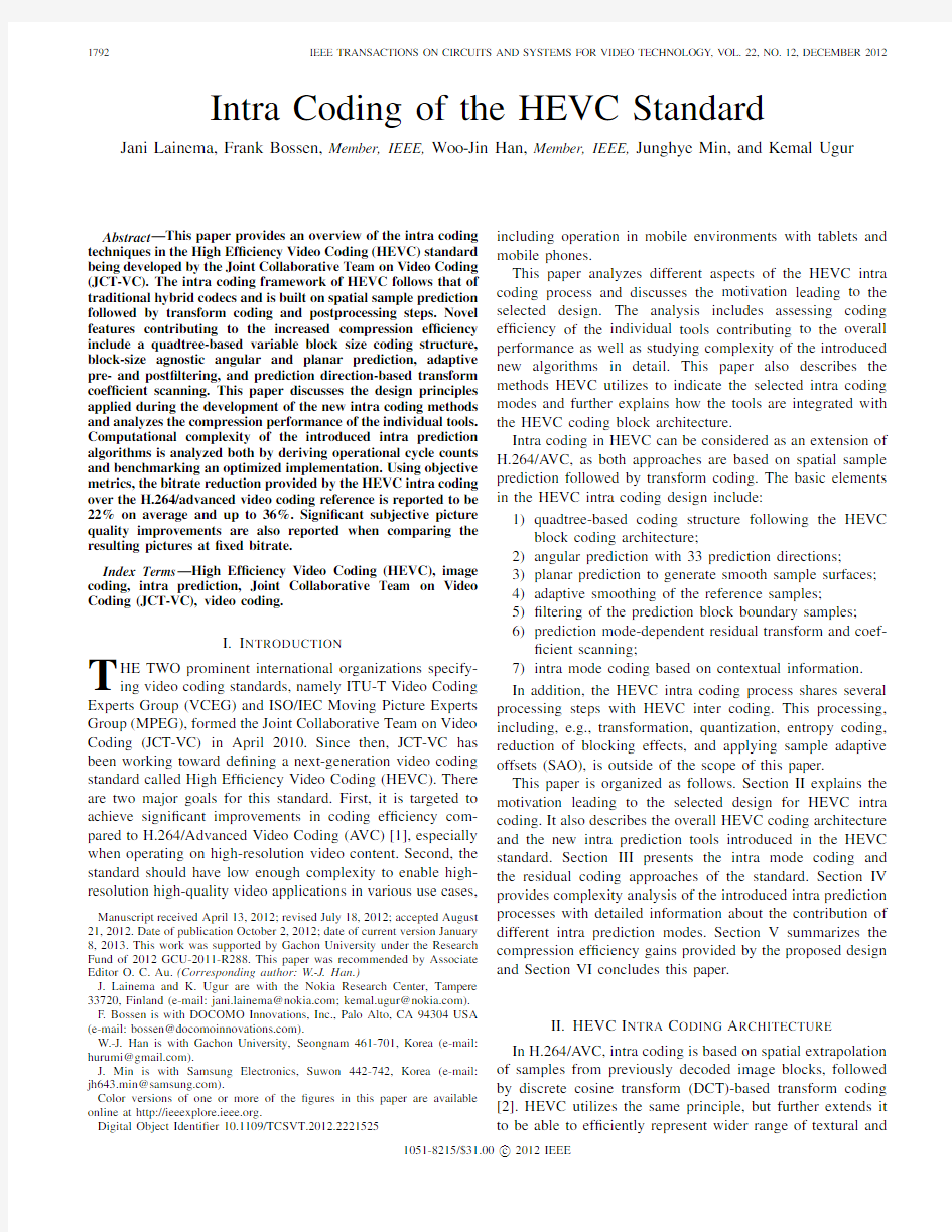
All the prediction modes utilize the same basic set of reference samples from above and to the left of the image block to be predicted.In the following sections,we denote the reference samples by R x,y with(x,y)having its origin one pixel above and to the left of the block’s top-left

corner.Fig.1.Reference samples R x,y used in prediction to obtain predicted samples P x,y for a block of size N×N samples.

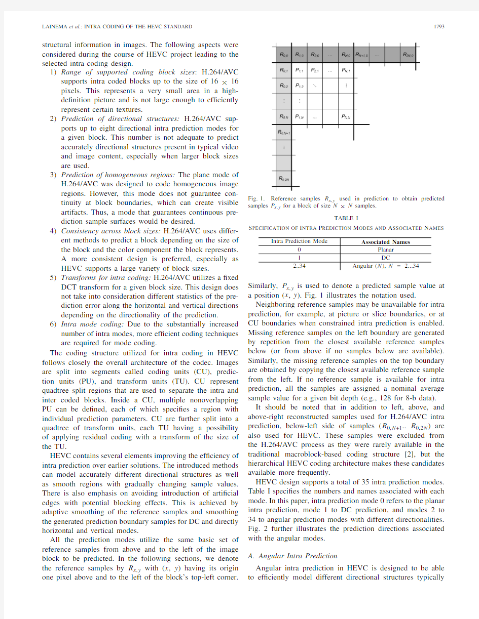
TABLE I

Specification of Intra Prediction Modes and Associated Names Intra Prediction Mode Associated Names

0Planar

1DC

2..34Angular(N),N=2 (34)

Similarly,P x,y is used to denote a predicted sample value at a position(x,y).Fig.1illustrates the notation used. Neighboring reference samples may be unavailable for intra prediction,for example,at picture or slice boundaries,or at CU boundaries when constrained intra prediction is enabled. Missing reference samples on the left boundary are generated by repetition from the closest available reference samples below(or from above if no samples below are available). Similarly,the missing reference samples on the top boundary are obtained by copying the closest available reference sample from the left.If no reference sample is available for intra prediction,all the samples are assigned a nominal average sample value for a given bit depth(e.g.,128for8-b data). It should be noted that in addition to left,above,and above-right reconstructed samples used for H.264/A VC intra prediction,below-left side of samples(R0,N+1..R0,2N)are also used for HEVC.These samples were excluded from the H.264/A VC process as they were rarely available in the traditional macroblock-based coding structure[2],but the hierarchical HEVC coding architecture makes these candidates available more frequently.

HEVC design supports a total of35intra prediction modes. Table I speci?es the numbers and names associated with each mode.In this paper,intra prediction mode0refers to the planar intra prediction,mode1to DC prediction,and modes2to 34to angular prediction modes with different directionalities. Fig.2further illustrates the prediction directions associated with the angular modes.

A.Angular Intra Prediction

Angular intra prediction in HEVC is designed to be able to ef?ciently model different directional structures typically

Fig.2.HEVC angular intra prediction modes numbered from2to34and the associated displacement parameters.H and V are used to indicate the horizontal and vertical directionalities,respectively,while the numeric part of the identi?er refers to the pixels’displacement as1/32pixel fractions. present in video and image contents.The number and angu-larity of prediction directions are selected to provide a good tradeoff between encoding complexity and coding ef?ciency for typical video material.The sample prediction process itself is designed to have low computational requirements and to be consistent across block sizes and prediction directions.The latter aims at minimizing the silicon area in hardware and the amount of code in software implementations.It is also intended to make it easier to optimize the implementation for high performance and throughput in various environments. This is especially important as the number of block sizes and prediction directions supported by HEVC intra coding far exceeds those of previous video codecs,such as H.264/A VC. In HEVC,there are four effective intra prediction block sizes ranging from4×4to32×32samples,each of which supports 33distinct prediction directions.A decoder must thus support 132combinations of block size and prediction direction. The following sections discuss in further detail different aspects contributing to the coding performance and implemen-tation complexity of the HEVC angular intra prediction.

1)Angle De?nitions:In natural imagery,horizontal and vertical patterns typically occur more frequently than patterns with other directionalities.The set of33prediction angles is de?ned to optimize the prediction accuracy based on this observation[7].Eight angles are de?ned for each octant with associated displacement parameters,as shown in Fig.2. Small displacement parameters for modes close to horizon-tal and vertical directions provide more accurate prediction for nearly horizontal and vertical patterns.The displacement parameter differences become larger when getting closer to diagonal directions to reduce the density of prediction modes for less frequently occurring

patterns.Fig.3.Example of projecting left reference samples to extend the top reference row.The bold arrow represents the prediction direction and the thin arrows the reference sample projections in the case of intra mode23 (vertical prediction with a displacement of?9/32pixels per row).

2)Reference Pixel Handling:The intra sample prediction process in HEVC is performed by extrapolating sample values from the reconstructed reference samples utilizing a given directionality.In order to simplify the process,all sample locations within one prediction block are projected to a single reference row or column depending on the directionality of the selected prediction mode(utilizing the left reference column for angular modes2to17and the above reference row for angular modes18to34).

In some cases,the projected pixel locations would have negative indexes.In these cases,the reference row or column is extended by projecting the left reference column to extend the top reference row toward left,or projecting the top reference row to extend the left reference column upward in the case of vertical and horizontal predictions,respectively.This approach was found to have a negligible effect on compression performance,and has lower complexity than an alternative approach of utilizing both top and left references selectively during the prediction sample generation process[5].Fig.3 depicts the process for extending the top reference row with samples from the left reference columns for an8×8block of pixels.

3)Sample Prediction for Arbitrary Number of Directions: Each predicted sample P x,y is obtained by projecting its location to a reference row of pixels applying the selected prediction direction and interpolating a value for the sample at1/32pixel accuracy.Interpolation is performed linearly utilizing the two closest reference samples

P x,y=

32?w y

·R i,0+w y·R i+1,0+16

>>5(1)

where w y is the weighting between the two reference samples corresponding to the projected subpixel location in between R i,0and R i+1,0,and>>denotes a bit shift operation to the right.Reference sample index i and weighting parameter w y are calculated based on the projection displacement d associated with the selected prediction direction(describing the tangent of the prediction direction in units of1/32samples

and having a value from ?32to +32as shown in Fig.2)as

c y =(y ·

d )>>5w y =(y ·d )&31i =x +c y

(2)

where &denotes a bitwise AND operation.It should be noted that parameters c y and w y depend only on the coordinate y and the selected prediction displacement d .Thus,both parameters remain constant when calculating predictions for one line of samples and only (1)needs to be evaluated per sample basis.When the projection points to integer samples (i.e.,when w y equals zero),the process is even simpler and consists of only copying integer reference samples from the reference row.Equations (1)and (2)de?ne how the predicted sample values are obtained in the case of vertical prediction (modes 18to 34)when the reference row above the block is used to derive the prediction.Prediction from the left reference column (modes 2to 17)is derived identically by swapping the x and y coordinates in (1)and (2).B.Planar Prediction

While providing good prediction in the presence of edges is important,not all image content ?ts an edge model.The DC prediction provides an alternative but is only a coarse approximation as the prediction is of order 0.H.264/A VC features an order-1plane prediction mode that derives a bilinear model for a block using the reference samples and generates the prediction using this model.One disadvantage of this method is that it may introduce discontinuities along the block boundaries.The planar prediction mode de?ned in HEVC aims to replicate the bene?ts of the plane mode while preserving continuities along block boundaries.It is essentially de?ned as an average of two linear predictions (see [8,Fig.2]for a graphical representation)

P V x,y =(N ?y )·R x,0+y ·R 0,N +1P H x,y =(N ?x )·R 0,y +x ·R N +1,0P x,y = P V

x,y +P H

x,y +N >> log 2(N )+1 .

(3)

C.Reference Sample Smoothing

H.264/A VC applies a three-tap smoothing ?lter to the ref-erence samples when predicting 8×8luma blocks.HEVC uses the same smoothing ?lter ([121]/4)for blocks of size 8×8and larger.The ?ltering operation is applied for each reference sample using neighboring reference samples.The ?rst reference sample R 0,2N and R 2N,0are not ?ltered.For 32×32blocks,all angular modes except horizontal and vertical use a ?ltered reference.In 16×16blocks,the modes not using a ?ltered reference are extended to the four modes (9,11,25,27)closest to horizontal and vertical.Smoothing is also applied where the planar mode is used,for block sizes 8×8and larger.However,HEVC is more discerning in the use of this smoothing ?lter for smaller blocks.For 8×8blocks,only the diagonal modes (2,18,34)use a ?ltered reference.Applying the reference sample smoothing selectively based on the block size and directionality of the prediction is reported to reduce contouring artifacts caused by edges in the reference sample arrays [23].

D.Boundary Smoothing

As noted above in the case of the H.264/A VC plane predic-tion mode,DC and angular prediction modes may introduce discontinuities along block boundaries.To remedy this prob-lem,the ?rst prediction row and column are ?ltered in the case of DC prediction with a two-tap ?nite impulse response ?lter (corner sample with a three-tap ?lter).Similarly,the ?rst prediction column for directly vertical prediction and the ?rst prediction row for directly horizontal prediction are ?ltered utilizing a gradient-based smoothing [9].For a more complete description of the ?ltering process,please refer to [25].

As the prediction for chroma components tends to be very smooth,the bene?ts of the boundary smoothing would be limited.Thus,in order to avoid extra processing with marginal quality improvements,the prediction boundary smoothing is only applied to luma component.The average coding ef?-ciency improvement provided by the boundary smoothing is measured to be 0.4%in HM 6.0environment [14].E.I

?

PCM Mode and Transform Skipping Mode

HEVC supports two special coding modes for intra coding denoted as I ?PCM and transform skipping mode.In I ?PCM mode,prediction,transform,quantization,and entropy coding are bypassed while the prediction samples are coded by a prede?ned number of bits.The main purpose of the I ?PCM mode is to handle the situation when the signal cannot be ef?ciently coded by other modes.

On the contrary,only transform is bypassed in transform skipping mode.It was adopted to improve the coding ef?-ciency for speci?c video contents such as computer-generated graphics.HEVC restricts the use of this mode when the block size is equal to 4×4to avoid the signi?cant design change due to this mode while this choice was proven to have most of coding ef?ciency bene?ts.F .Restrictions for Partitioning Types

HEVC intra coding supports two types of PU division,PART ?2N ×2N and PART ?N ×N ,splitting a CU into one or four equal-size PUs,respectively.However,the four regions speci?ed by the partitioning type PART ?N ×N can be also represented by four smaller CU with the partitioning type PART ?2N ×2N .Due to this,HEVC allows an intra CU to be split into four PU only at the minimum CU size.It has been demonstrated that this restriction is associated with minimal impact in coding ef?ciency,but it reduces the encoding complexity signi?cantly [3].

Another way to achieve the same purpose would be reducing the CU size to 4×4with the partitioning mode PART ?2N ×2N .However,this approach would result in a chroma intra prediction block size of 2×2pixels,which can be critical to the throughput of the entire intra prediction process.For this reason,the minimum allowed CU size is restricted to 8×8pixels while allowing the partitioning type PART ?N ×N only in the smallest CU.G.TU-Based Prediction

When a CU is split into multiple TU,the intra prediction is applied for each TU sequentially instead of applying the

intra prediction at the PU level.One obvious advantage for this approach is the possibility of always utilizing the nearest neighboring reference samples from the already reconstructed TU.It has been shown that this property improves the intra picture coding ef?ciency by about1.2%[4]compared to the case of using PU border reference samples for the PU.It should be noted that all the intra prediction information is indicated per PU and the TUs inside the same PU share the same intra prediction mode.

III.Mode and Residual Coding

A.Mode Coding for Luma

HEVC supports total33angular prediction modes as well as planar and DC prediction for luma intra prediction for all the PU sizes.Due to the large number of intra prediction modes, H.264/A VC-like mode coding approach based on a single most probable mode was not found effective in HEVC[8].Instead, HEVC de?nes three most probable modes for each PU based on the modes of the neighboring PUs.The selected number of most probable modes makes it also possible to indicate one of the32remaining modes by a?xed length code,as the distribution of the mode probabilities outside of the set of most probable modes is found to be relatively uniform.

The selection of the set of three most probable modes is based on modes of two neighboring PUs,one above and one to the left of the current PU.By default,modes of both candidate PUs are included in the set.Possible duplicates and the third mode in the set are assigned with modes planar,DC,or angular (26)in this order.In the case that both top and left PU has the same directional mode,that mode and two closest directional modes are used to construct the set of most probable modes instead.

In the case current intra prediction mode is equal to one of the elements in the set of most probable modes,only the index in the set is transmitted to the decoder.Otherwise,a5-b?xed length code is used to determine the selected mode outside of the set of most probable modes.

B.Derived Mode for Chroma Intra Prediction

Quite often structures in the chroma signal follow those of the luma.Taking advantage of this behavior,HEVC introduces a mechanism to indicate the cases when chroma PU utilizes the same prediction mode as the corresponding luma PU.Table II speci?es the mode arrangement used in signaling the chroma mode.

In the case that derived mode is indicated for a PU,the prediction is performed by using the corresponding luma PU mode.In order to remove the possible redundancy in the signaling arising when derived refers to one of the modes always present,angular(34)mode is used to substitute the duplicate mode as shown in Table II.

C.Syntax Design for the Intra Mode Coding

HEVC uses three syntax elements to represent the luma intra prediction mode.The syntax element prev?intra?luma?pred??ag speci?es whether the luma intra

TABLE II

Specification of Chroma Intra Prediction

Modes and Associated Names

Chroma intra Alternative mode,if

prediction Primary mode primary mode is equal to

mode the derived mode

0Planar Angular(34)

1Angular(26)Angular(34)

2Angular(10)Angular(34)

3DC Angular(34)

4Derived N/A prediction mode is matched with one of three most probable modes.When the?ag is equal to1,the syntax element mpm?idx is parsed,indicating which element of the most probable mode array speci?es the luma intra prediction mode.When the?ag is equal to0,the syntax element rem?intra?luma?pred?mode is parsed,specifying the luma intra prediction mode as rem?intra?luma?pred?mode+N, where N is the number of elements in the most probable mode array having a mode index greater than or equal to the syntax element rem?intra?luma?pred?mode.

In chroma mode coding,a1-b syntax element(0)is assigned to the most often occurring derived mode,while3-b syntax elements(100,101,110,111)are assigned to the remaining four modes.

D.Intra Mode Residual Coding

HEVC utilizes intra mode dependent transforms and co-ef?cient scanning for coding the residual information.The following sections describe the selected approaches in more detail.

1)Block Size-Dependent Transform Selection:Integer trans-forms derived from DCT and discrete sine transform(DST)are applied to the intra residual blocks.A DST-based transform is selected for4×4luma blocks and DCT-based transforms for the rest.For more details on the speci?cation of the transforms, the reader is referred to[10]and[11].

Different approaches to select the transforms were studied during the course of the HEVC development.For example, an early HEVC draft utilized a method that selected the horizontal and vertical transforms separately for4×4luma blocks based on the intra prediction mode.This approach provided an average coding ef?ciency improvement of0.8% [10].However,it was found that the simple block size de-pended approach now adopted in the standard provides very similar coding ef?ciency[26].Also larger size alternative transforms were studied,but it was reported that the additional coding ef?ciency improvements were marginal compared to the complexity impact[27].Thus,only DCT-based transforms are utilized for block sizes larger than4×4.

2)Intra Prediction Mode-Dependent Coef?cient Scanning: HEVC applies adaptive scanning of transform coef?cients to the transform block sizes of4×4and8×8in order to take advantage of the statistical distribution of the active coef?cients in2-D transform blocks.The scan is selected based on directionality of the intra prediction mode as shown

TABLE III

Mapping Table Between Intra Prediction Modes and Coefficient Scanning Order

Intra Coef?cient Coef?cient

prediction mode

scanning for scanning for

4×4and8×816×16and32×32

Angular(6–14)Vertical Diagonal

Angular(22–30)Horizontal Diagonal

All other modes Diagonal Diagonal

in Table III.Vertical and horizontal scans refer to the cor-

responding raster scan orders,while the diagonal scan refers

to a diagonal scan from down-left to up-right direction.The

average coding gain from the intra mode dependent scans is

reportedly around1.2%[12].

https://www.360docs.net/doc/871184343.html,plexity of Intra Prediction Tools

https://www.360docs.net/doc/871184343.html,plexity Analysis of Decoding Process

1)Analysis of Operational Cycle Counts:De?ning a proper

metric for theoretical analysis of complexity can be dif?cult

as various aspects come into play.For example,if relying on

counting operations,de?ning what constitutes one operation

largely depends on the underlying architecture.The bit width

of each data element being processed also plays an important

role in determining a number of gates in hardware and

the amount of parallelism achievable in software.How an

algorithm is implemented can also have a signi?cant impact.

A lower number of operations is not always better.Executing

four operations in parallel may be faster and considered less

complex than executing three in sequence.In this section,we

thus limit ourselves to a more super?cial comparison of HEVC

prediction modes with the H.264/A VC ones.

The DC,directly horizontal,and directly vertical predic-

tion modes are the ones most similar to those de?ned in

H.264/A VC.HEVC simply de?nes an additional post?ltering

operation where one row and/or column of samples is?ltered.

The overhead of such?ltering becomes less with larger block

sizes,as the fraction of?ltered samples becomes smaller.

For predicting a block of size N×N,angular prediction

requires the computation of p=(u·a+v·b+16)>>5for

each sample,which involves two multiplications(8-b unsigned

operands,16-b result),two16-b additions,and one16-b shift

per predicted sample,for a total of?ve operations.In the

H.264/A VC case,directional prediction may take the form

p=(a+2b+c+2)>>2,which may be considered to be ?ve operations as well.However,on some architectures,this

can be implemented using two8-b halving add operations:

d=(a+c)>>1and p=(d+b+1)>> 1.The H.264/A VC directional prediction process is thus less complex as it requires no multiplication and no intermediate value wider than9b.

In the case of the plane and planar modes,considering

the generating equations is probably not adequate,as the

prediction values can be ef?ciently computed incrementally.

For the H.264/A VC plane mode,it is expected that one16-b

addition,one16-b shift,and one clip to8-b range are required

TABLE IV

Decoding Time Comparison Between HM6.0Decoder and Its Optimized Decoder Used for Further Analysis

Setting

Bitrate HM6.0Optimized

(Mbit/s)(s)(s) BasketballDrive,QP=2271.1104.4721.97

BasketballDrive,QP=378.461.60 6.98

BQTerrace,QP=22179.2163.9441.42

BQTerrace,QP=3721.691.0012.03

Cactus,QP=22105.7120.4628.84

Cactus,QP=3714.269.598.78

Kimono,QP=2222.337.117.02

Kimono,QP=37 3.826.94 2.88

ParkScene,QP=2252.760.5314.02

ParkScene,QP=377.333.90 4.35

Geometric mean25.466.3410.91

Sequences are each10-s long and are coded in intra-only mode.Optimized decoder is about four to nine times faster than HM.

per sample.For the HEVC planar mode,three16-b additions and one16-b shift are expected per sample.

The partial analysis provided here is indicative.It suggests that the HEVC intra prediction modes are more complex than the A VC modes,but not necessarily by a large amount.In the following,focus is shifted to complexity investigation based on actual implementations.

2)Decoding Time of Intra Prediction in Relation to Overall Decoding Time:In a?rst experiment,the percentage of de-coding time spent on intra prediction is measured.Reference encodings for the main pro?le of HM6.0[14]are used in the all-intra con?guration[15].The experiment is focused on high-de?nition sequences from the JCT-VC class B test set(?ve 1920×1080sequences).MD5checksum computation and ?le output of the reconstructed pictures are disabled such that decoding times more accurately re?ect time spent on actually decoding pictures.Measurements are obtained on a laptop featuring an Intel Core i5processor clocked at 2.53GHz. Software was compiled using gcc4.6.3.In addition to the HM software,an optimized decoder,based on[16],is also considered.Table IV summarizes decoding times and gives an indication of the level of optimization.For the comparative results between HEVC HM decoder and H.264/A VC JM decoder,please refer to[24],which reported that they are comparable.The fraction of decoding time used for intra prediction is further summarized in Table V.

While the results obtained with HM and optimized software show some differences,they do not diverge signi?cantly:on average roughly12%–15%of decoding time is consumed by intra prediction.The results may however be somewhat surprising in the sense that generating the reference arrays used for prediction takes more time than generating the prediction from those reference arrays.Part of this observation may be caused by the fact that in both of the tested software implemen-tations,full reference arrays are constructed,including2N+1 samples for a row above and2N+1samples for a left column. Most prediction modes do not require all these samples,and constructing only the required ones may reduce the amount of time by up to50%.

TABLE V

Decoding Time Fraction for Intra Prediction

Setting Reference Prediction Total (%)(%)(%)

BasketballDrive,QP=2211.0/5.7 5.0/3.815.0/9.5 BasketballDrive,QP=379.9/8.0 5.7/9.415.6/17.4 BQTerrace,QP=2210.2/4.6 4.2/2.514.4/7.1 BQTerrace,QP=3711.6/8.3 6.3/7.117.9/15.4 Cactus,QP=2210.6/5.4 4.5/3.215.1/8.6 Cactus,QP=3711.1/8.8 5.5/8.016.6/16.8 Kimono,QP=228.3/4.5 4.3/4.912.6/9.4 Kimono,QP=378.0/6.6 5.0/8.813.0/15.4 ParkScene,QP=2210.1/5.4 4.3/2.914.4/8.3 ParkScene,QP=3710.8/8.2 5.0/7.115.8/15.3 Average10.2/6.6 5.0/5.815.2/12.4 Reference represents construction of the reference samples array and Prediction represents the actual prediction process.For the HM6software, functions in the TComPattern class are considered part of reference, functions in the TComPrediction class part of prediction.In each pair of numbers,the left one represents HM6and the right one the optimized decoder

TABLE VI

Cycles Per Sample for Intra Prediction Modes(in a Specific Software Implementation Based on[16])

Luma Chroma

Mode4816324816 DC 1.500.750.440.220.280.140.08 Planar 1.130.660.650.640.560.450.50 Horizontal0.940.420.190.120.380.230.20 Vertical0.940.520.320.260.280.120.10 Angular(2–9) 1.31 1.230.820.68 1.130.730.67 Angular(11–17) 1.50 1.230.890.69 1.410.830.67 Angular(18–25) 1.50 1.140.760.56 1.310.710.63 Angular(27–34) 1.31 1.140.780.55 1.130.730.61 3)Cycles for Each Prediction Mode:Using optimized software based on[16],the decoding time associated with each prediction mode is further studied.Table VI shows numbers of computed cycles,normalized by the number of predicted samples.Numbers for chroma are reported separately for two reasons:post?ltering is not applied to chroma components (DC,horizontal,and vertical modes)and predictions for both chroma components can be generated concurrently.Note that the number of cycles may vary for different angular prediction modes.Angular modes are thus split into four categories (positive/negative angle,main direction is hor/ver).

Note that the cost of DC postsmoothing is signi?cant. For blocks of size4×4,the DC mode even is the most time-consuming prediction mode.It should be further noted that the postsmoothing is not optimized by SIMD opera-tions(at least not manually).While the number of cycles per sample decreases as the size of the blocks increase, this does not always seem to be the case.The differences between the various angular ranges are due to two factors:for modes2–9and11–17,the result is transposed,leading to a higher cycle count;and for modes11–17and18–25,samples from the second reference array are projected onto the?rst one.

TABLE VII

Results of the Tests on Different Intra Coding Tools

Test1Test2Test3Test4Test5 Class BDR BDR BDR BDR BDR

Class A 6.1% 5.7% 2.6%9.6% 1.1%

Class B 6.5%8.5% 1.5% 5.7% 1.0%

Class C 6.9% 3.7%0.3% 1.6% 1.1%

Class D 4.8% 2.5%0.3% 1.4%0.8%

Class E9.5%12.3% 1.9% 6.9% 1.6%

Class F 5.6% 4.8%0.3% 1.5% 1.2%

Maximum14.8%19.2% 4.7%16.3% 1.6% All 6.5% 6.1% 1.1% 4.4% 1.1%

B.Fast Encoding Algorithm

While an increase in the number of intra prediction modes

can provide substantial performance gains,it also makes the

rate-distortion(RD)optimization process more complex.In

this section,we introduce the new encoding algorithm utilized

by the of?cial HM6.0reference software and describe how it

is optimized for large sets of prediction candidates[17].

The fast encoding algorithm of HM software includes two

phases.In the?rst phase,the N most promising candidate

modes are selected by the rough mode decision process.In this

process,all candidates(35modes)are evaluated with respect

to the following cost function:

C=D Had+λ·R mode(4) where the D Had represents the absolute sum of Hadamard

transformed residual signal for a PU and R mode represents the

number of bits for the prediction mode.

In the second stage,the full RD costs with reconstructed

residual signal used for actual encoding process are compared

among the N best candidates.The prediction mode with the

minimum RD cost is selected as the?nal prediction mode.The

number N is varied depending on the PU size.The N is set to {8,8,3,3,3}for4×4,8×8,16×16,32×32,and64×64 PU,respectively,to allow more thorough search for the small

block sizes most critical to the joint optimization of prediction

and residual data.It should be noted that the size of TU is

assumed to be equal to the maximum possible value rather

than allowing the TU splitting in this stage for minimizing the

complexity.RD optimized TU structure is determined after the

second stage by using the best prediction mode.

Results marked as Test6in Table VIII indicate that the

design of the described fast algorithm is well optimized for

the large number of prediction modes.

V.Experimental Results

A.Test Conditions

The JCT-VC common test conditions[20]were used to

evaluate the performance of different aspects of the intra

picture coding of HEVC.These conditions de?ne a set of24

video sequences in six classes(A to F)covering a wide range

of resolutions and use cases.In addition to natural camera

captured material,the Class F sequences also include computer

screen content and computer graphics content,as well as

TABLE VIII

Results of the Tests on Fast Intra Encoding and SAO

Test6Test7

Class BDR t(enc) BDR

Class A?0.4%294%0.8%

Class B?0.3%296%0.7%

Class C?0.3%297%0.9%

Class D?0.4%296%0.6%

Class E?0.4%286%0.9%

Class F?0.4%303% 2.9%

Maximum?0.2%333% 4.3%

All?0.4%296% 1.1%

content mixing natural video and graphics.In order to assess the objective quality differences,Bj?ntegaard delta bitrates are computed using piece-wise cubic interpolation[18],[19]. The10-b Nebuta and SteamLocomotive sequences were not included in the experimental results since the HEVC Main pro?le only speci?es operation for8-b4:2:0video.

HM6.0reference software[14]with the Main pro?le set-tings were used to evaluate the HEVC intra coding perfor-mance.The four rate points required to calculate the Bj?n-tegaard delta bitrates were generated by using quantization parameters22,27,32,and37.

Performance of the H.264/A VC intra coding was investi-gated using JM18.2reference software[22]with its high-pro?le settings(RD optimizations,8×8DCT and CABAC enabled).In order to operate approximately at the same bitrates with HEVC,quantization parameters of24,29,34,and39 were used for H.264/A VC.

B.Experimental Results

2)Performance Analysis of the HEVC Intra Coding Tools: In order to analyze how different aspects contribute to the total performance of HEVC intra coding,the following experiments were carried out.

1)Test1:Restricting HM6.0intra modes to the eight

H.264/A VC directional modes,DC,and planar mode,

utilizing a1-MPM approach for mode coding.

2)Test2:Restricting the HM6.0maximum CU size to

16×16and the maximum TU size to8×8.

3)Test3:Restricting the maximum TU size to16×16.

4)Test4:Restricting the maximum TU size to8×8.

5)Test5:Substituting the HM6.03-MPM intra mode

coding with a1-MPM approach.

6)Test6:Utilizing full RD optimizations for selecting the

intra mode as described in Section IV-B.

7)Test7:Switching off SAO.

The relevant syntax changes due to the differences of the number of intra modes and MPMs were applied in Tests1 and5for the fair comparison.Tables VII and VIII summa-rize the performance for each test.Positive numbers indicate the increase in bitrate associated with restricting the codec according to the test descriptions.In addition to the average and per class results,the maximum difference for a single test sequence is also reported.According to Test1,the average impact provided by the HEVC angular prediction is6.5%

TABLE IX

Performance of HM6.0Compared With JM18.2

Class Sequence Bit-saving(%) Class A(2560×1600)Traf?c?21.9

PeopleOnStreet?22.2

Kimono?27.8

ParkScene?16.5 Class B(1920×1080)Cactus?23.6

BasketballDrive?29.0

BQTerrace?20.8

BasketballDrill?31.7

BQMall?20.3 Class C(832×480)PartyScene?12.6

RaceHorses?18.3

BasketballPass?22.6

BQSquare?13.3 Class D(416×240)BlowingBubbles?13.8

RaceHorses?19.3

FourPeople?23.3 Class E(1280×720)Johnny?35.5

KristenAndSara?28.8

BasketballDrillText?27.9 Class F(1024×768)ChinaSpeed?18.8

SlideEditing?15.7

SlideShow?27.6

Class A?22.1

Class B?23.6

Class C?20.7

Class D?17.2 Averages Class E?29.2

Class F?22.5

Maximum?35.5

All?22.3 while more differences up to14.8%are noticed for sequences with strong directional patterns such as BasketballDrive and BasketballDrill.In addition,the coding ef?ciency bene?ts are rather uniform across difference classes while Class E,which consists of the video conferencing sequences having large objects and steady background,provides more bene?ts. Allowing larger CU,PU,and TU with more?exibility in both predicting and transforming the picture content provides an average bitrate impact of6.1%according to Test2.To clarify further,Tests3and4study the effects provided by utilization of transform sizes larger than8×8while keeping the maximum CU size to64×64.Test3indicates that switch-ing of the32×32transform affects the coding ef?ciency by 1.1%on average and Test4indicates that switching off both 32×32and16×16transforms has an average impact of 4.4%.It can be observed that the coding ef?ciency bene?ts from the large size transform become more signi?cant when the spatial resolution of the video sequence is increased.Test 5shows that using one most probable mode instead of three would result in1.1%average coding ef?ciency difference. Test6illustrates the performance of the HM6.0encoding algorithm for intra coding.A full RD optimized codec would be able to achieve a?0.4%coding gain on average,but with almost three times the encoding time of HM6.0.Thus,the current HM6.0encoder design seems to provide a very inter-esting compromise between coding ef?ciency and complexity.

Fig.4.Example of visual quality improvements in 50f/s BasketballDrive 1920×1080sequence.(a)HM 6.0(8.4Mb/s).(b)A VC 10modes (8.5Mb/s).(c)JM 18.2(9.1

Mb/s).

Fig.5.Example of visual quality improvements in the ?rst frame of 60f/s KristenAndSara 1280×720sequence.Above:an extract of HM 6.0coded frame at 4.8Mb/s.Below:JM 18.2at 4.9Mb/s.

Finally,Test 7provides the results showing that the switching off SAO results in the 1.1%coding ef?ciency loss on average.2)Performance Compared to H.264/AVC Intra Coding :Table IX compares the intra picture coding performance of HEVC with that if H.264/A VC using the test conditions described above.The experiment indicates that in order to achieve similar objective quality,HEVC needs 22.3%lower bitrate on average.Although the average bit-saving of HEVC intra coding seems less than that of HEVC inter coding,which was typically reported over 30%,the bene?ts are still substantial.

The advantages over H.264/A VC intra coding tend to be larger when the video resolution becomes higher and the strong directionalities exist.Differences close to 30%were observed for seven of the sequences:Kimono,BasketballDrive,BasketballDrill,Johnny,KristenAndSara,BasketballDrillText ,and SlideShow .The highest difference of 35.5%is obtained in the case of Johnny .These sequences are characterized by strong directional textures.In addition,Kimono,Johnny ,and KristenAndSara feature also large homogenous regions.The ?exible coding structure of HEVC supporting blocks up to 64×64with accurate prediction means appears to be espe-cially effective for this kind of content.The large transform block size also plays a role in performance improvement by

providing strong energy compaction and smaller quantization errors.Especially for regions that cannot be properly predicted by angular prediction (e.g.,diverse textures),a large transform is successfully applied for residual coding.Sample-adaptive offset ?ltering also provides additional gains in intra pictures by compensating distortions between reconstructed and origi-nal signals.

3)Subjective Quality Evaluation :Comparison of visual quality provided by HM 6.0implementation of HEVC,HM 6.0restricted to 10intra prediction modes as described for Test 1above,and JM 18.2implementation of H.264/A VC is presented in Fig.4.It shows that directional patterns are much more clear and distinctive in the image produced by HM 6.0while blurred lines are observed in other cases.In the image from the JM,several lines are completely missing.Very similar effects are noticeable also in Fig.5,comparing decoded picture quality of HM 6.0with that of JM 18.2in the case of the KristenAndSara test sequence.It appears that the angular prediction with accurate prediction directions contribute positively to the reconstruction of edge structures.As can be observed from these results,the angular prediction and other intra tools adopted in HM 6.0have potential to provide signi?cant improvements in visual quality in addition to the objective performance gains.

VI.Conclusion

The intra coding methods described in this paper can provide signi?cant improvements in both objective and subjective quality of compressed video and still pictures.While demonstrating compression ef?ciency superior to previous solutions,computational requirements and different aspects affecting implementation in various environments were thoroughly considered.The proposed methods passed stringent evaluation by the JCT-VC community and now form the intra coding toolset of the HEVC standard.Potential future work in the area includes,e.g.,extending and tuning the tools for multiview/scalable coding,higher dynamic range operation,and 4:4:4sampling formats.

Acknowledgment

The authors would like to thank the experts of ITU-T VCEG,ISO/IEC MPEG,and the ITU-T/ISO/IEC Joint Col-laborative Team on Video Coding for their contributions and collaborative spirit.

References

[1]Advanced Video Coding for Generic Audiovisual Services ,ISO/IEC

14496-10,ITU-T Rec.H.264,Mar.2010.

[2]T.Wiegand,G.J.Sullivan,G.Bj?ntegaard,and A.Luthra,“Overview

of the H.264/A VC video coding standard,”IEEE Trans.Circuits Syst.Video Technol.,vol.13,no.7,pp.560–576,Jul.2003.

[3]J.Kim and B.Jeon,Encoding Complexity Reduction by Removal of

N ×N Partition Type,JCTVC-D087,Daegu,Korea,Jan.2011.

[4]T.Lee,J.Chen,and W.-J.Han,TE 12.1:Transform Unit Quadtree/2-Level Test,JCTVC-C200,Guangzhou,China,Oct.2010.

[5]T.K.Tan,M.Budagavi,and https://www.360docs.net/doc/871184343.html,inema,Summary Report for TE5on

Simpli?cation of Uni?ed Intra Prediction,JCTVC-C046,Guangzhou,China,Oct.2010.

[6]K.Ugur,K.R.Andersson,and A.Fuldseth,Video Coding Technology

Proposal by Tandberg,Nokia,and Ericsson,JCTVC-A119,Dresden, Germany,Apr.2010.

[7]J.Min,S.Lee,I.Kim,W.-J.Han,https://www.360docs.net/doc/871184343.html,inema,and K.Ugur,Uni?cation

of the Directional Intra Prediction Methods in TMuC,JCTVC-B100, Geneva,Switzerland,Jul.2010.

[8]S.Kanumuri,T.K.Tan,and F.Bossen,Enhancements to Intra Coding,

JCTVC-D235,Daegu,Korea,Jan.2011.

[9] A.Minezawa,K.Sugimoto,and S.Sekiguchi,An Improved Intra

Vertical and Horizontal Prediction,JCTVC-F172,Torino,Italy,Jul.

2011.

[10] A.Saxena and F. C.Fernandes,CE7:Mode-Dependent DCT/DST

Without4*4Full Matrix Multiplication for Intra Prediction,JCTVC-E125,Geneva,Switzerland,Mar.2011.

[11]R.Joshi,P.Chen,M.Karczewicz,A.Tanizawa,J.Yamaguchi,C.Yeo,

Y.H.Tan,H.Yang,and H.Yu,CE7:Mode Dependent Intra Residual Coding,JCTVC-E098,Geneva,Switzerland,Mar.2011.

[12]Y.Zheng,M.Coban,X.Wang,J.Sole,R.Joshi,and M.Karczewicz,

CE11:Mode Dependent Coef?cient Scanning,JCTVC-D393,Daegu, Korea,Jan.2011.

[13]V.Sze,K.Panusopone,J.Chen,T.Nguyen,and M.Coban,CE11:

Summary Report on Coef?cient Scanning and Coding,JCTVC-D240, Daegu,Korea,Jan.2011.

[14]HM 6.0Reference Software[Online].Available:http://hevc.kw.bbc.

https://www.360docs.net/doc/871184343.html,/trac/browser/tags/HM-6.0

[15]HM6.0Anchor Bitstreams[Online].Available:ftp://https://www.360docs.net/doc/871184343.html,/

hevc/hm-6.0-anchors/

[16] F.Bossen,On Software Complexity,HM 6.0Reference Software,

JCTVC-G757,Geneva,Switzerland,Nov.2011.

[17]Y.Piao,J.Min,and J.Chen,Encoder Improvement of Uni?ed Intra

Prediction,JCTVC-C207,Guangzhou,China,Oct.2010.

[18]G.Bj?ntegaard,Calculation of Average PSNR Differences Between RD-

Curves,VCEG-M33,Austin,TX,Apr.2001.

[19]G.Bj?ntegaard,Improvement of BD-PSNR Model,VCEG-AI11,Berlin,

Germany,Jul.2008.

[20] F.Bossen,Common Test Conditions,JCTVC-H1100,San Jose,CA,Mar.

2012.

[21]K.McCann,W.-J.Han,I.Kim,J.Min,E.Alshina,A.Alshin,T.Lee,J.

Chen,V.Seregin,S.Lee,Y.Hong,M.Cheon,and N.Shlyakhov,Video Coding Technology Proposal by Samsung,JCTVC-A124,Dresden,Ger-many,Apr.2010.

[22]JM18.2Reference Software[Online].Available:http://iphome.hhi.de/

suehring/tml/download

[23]M.Wien,“Variable block-size transform for H.264/A VC,”IEEE Trans.

Circuits Syst.Video Technol.,vol.13,no.7,pp.604–619,Jul.2003.

[24]G.J.Sullivan and J.Xu,Comparison of Compression Performance of

HEVC Working Draft5with AVC High Pro?le,JCTVC-H0360,San Jose,CA,Feb.2012.

[25] B.Bross,W.-J.Han,G.J.Sullivan,J.-R.Ohm,and T.Wiegand,

High Ef?ciency Video Coding(HEVC)Text Speci?cation Draft7, ITU-T/ISO/IEC Joint Collaborative Team on Video Coding(JCT-VC) document JCTVC-I1003,May2012.

[26]K.Ugur and A.Saxena,CE1:Summary Report of Core Experiment

on Intra Transform Mode Dependency Simpli?cations,JCTVC-J0021, Stockholm,Sweden,Jul.2012.

[27]R.Cohen,C.Yeo,R.Joshi,and F.Fernandes,CE7:Summary Report of

Core Experiment on Additional Transforms,document JCTVC-H0037,

San Jose,CA,Feb.

2012.

Jani Lainema received the M.Sc.degree in com-puter science from the Tampere University of Tech-nology,Tampere,Finland,in1996.

Since1996,he has been with the Visual Commu-nications Laboratory,Nokia Research Center,Tam-pere,where he contributes to the designs of ITU-T’s and MPEG’s video coding standards as well as to the evolution of different multimedia service standards in3GPP,DVB,and DLNA.He is currently a Prin-cipal Scientist with Visual Media,Nokia Research Center.His current research interests include video,

image,and graphics coding and communications,and practical applications of game theory.Frank Bossen(M’04)received the M.Sc.degree in computer science and the Ph.D.degree in communication systems from the Ecole Polytechnique Fédérale de Lausanne,Lausanne,Switzerland,in1996and1999,respectively.

He has been active in video coding standardization since1995and has held a number of positions with IBM,Yorktown Heights,NY;Sony,Tokyo, Japan;GE,Ecublens,Switzerland;and NTT DOCOMO,San Jose,CA.He is currently a Research Fellow with DOCOMO Innovations,Inc.,Palo Alto,

CA.

Woo-Jin Han(M’02)received the M.S.and Ph.D.

degrees in computer science from the Korea Ad-

vanced Institute of Science and Technology,Dae-

jeon,Korea,in1997and2002,respectively.

He is currently a Professor with the Department

of Software Design and Management,Gachon Uni-

versity,Seongnam,Korea.From2003to2011,he

was a Principal Engineer with the Multimedia Plat-

form Laboratory,Digital Media and Communication

Research and Development Center,Samsung Elec-

tronics,Suwon,Korea.Since2003,he has been contributing successfully to the ISO/IEC Moving Pictures Experts Group, Joint Video Team,and Joint Collaborative Team standardization effort. His current research interests include high ef?ciency video compression techniques,scalable video coding,multiview synthesis,and visual contents understanding.

Dr.Han was an editor of the HEVC video coding standard in

2010.

Junghye Min received the B.S.degree in mathemat-

ics from Ewha Women’s University,Seoul,Korea,in

1995,and the M.E.and Ph.D.degrees in computer

science and engineering from Pennsylvania State

University,University Park,PA,in2003and2005,

respectively.

From1995to1999,she was a S/W Engineer

with Telecommunication Systems Business,Sam-

sung Electronics,Suwon,Korea.She is currently

a Principal Engineer with the Multimedia Platform

Laboratory,Digital Media and Communications Re-search and Development Center,Samsung Electronics,Suwon.Her current research interests include video content analysis,motion tracking,pattern recognition,and video

coding.

Kemal Ugur received the M.Sc.degree in electrical

and computer engineering from the University of

British Columbia,Vancouver,BC,Canada,in2004,

and the Doctorate degree from the Tampere Univer-

sity of Technology,Tampere,Finland,in2010.

Currently,he is a Research Leader with the Nokia

Research Center,Tampere,working on the devel-

opment of next-generation audiovisual technologies

and standards.Since joining Nokia,he has actively

participated in several standardization forums,such

as the Joint Video Team’s(JVT)work on the stan-dardization of the multiview video coding extension of H.264/MPEG-4A VC, and the Video Coding Experts Group’s(VCEG)explorations toward a next-generation video coding standard,the3GPP activities for mobile broadcast and multicast standardization,and recently,the Joint Collaborative Team on Video Coding(JCT-VC)for development of high ef?ciency video coding (HEVC)standard.He has authored more than30publications in academic conferences and journals and has over40patents pending.

Dr.Ugur is a member of the research team that received the Nokia Quality Award in2006.