Adaptive Restart for Accelerated Gradient Schemes

Found Comput Math(2015)15:715–732

DOI10.1007/s10208-013-9150-3

Adaptive Restart for Accelerated Gradient Schemes

Brendan O’Donoghue·Emmanuel Candès

Received:2January2013/Accepted:25February2013/Published online:3July2013

?SFoCM2013

Abstract In this paper we introduce a simple heuristic adaptive restart technique that can dramatically improve the convergence rate of accelerated gradient schemes.The analysis of the technique relies on the observation that these schemes exhibit two modes of behavior depending on how much momentum is applied at each iteration. In what we refer to as the‘high momentum’regime the iterates generated by an accel-erated gradient scheme exhibit a periodic behavior,where the period is proportional to the square root of the local condition number of the objective function.Separately, it is known that the optimal restart interval is proportional to this same quantity.This suggests a restart technique whereby we reset the momentum whenever we observe periodic behavior.We provide a heuristic analysis that suggests that in many cases adaptively restarting allows us to recover the optimal rate of convergence with no prior knowledge of function parameters.

Keywords Convex optimization·First order methods·Accelerated gradient schemes

Mathematics Subject Classi?cation80M50·90C06·90C25

Communicated by Felipe Cucker.

B.O’Donoghue(B)·E.Candès

Stanford University,450Serra Mall,Stanford,CA94305,USA

e-mail:bodonoghue85@https://www.360docs.net/doc/8e6212838.html,

E.Candès

e-mail:candes@https://www.360docs.net/doc/8e6212838.html,

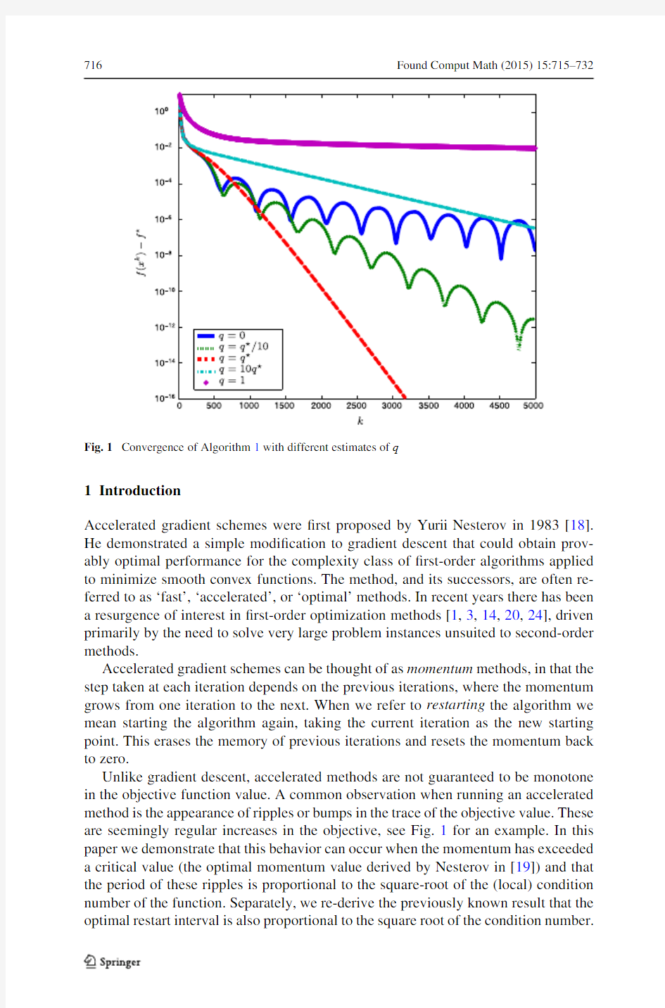
Fig.1Convergence of Algorithm1with different estimates of q

1Introduction

Accelerated gradient schemes were?rst proposed by Yurii Nesterov in1983[18]. He demonstrated a simple modi?cation to gradient descent that could obtain prov-ably optimal performance for the complexity class of?rst-order algorithms applied to minimize smooth convex functions.The method,and its successors,are often re-ferred to as‘fast’,‘accelerated’,or‘optimal’methods.In recent years there has been a resurgence of interest in?rst-order optimization methods[1,3,14,20,24],driven primarily by the need to solve very large problem instances unsuited to second-order methods.

Accelerated gradient schemes can be thought of as momentum methods,in that the step taken at each iteration depends on the previous iterations,where the momentum grows from one iteration to the next.When we refer to restarting the algorithm we mean starting the algorithm again,taking the current iteration as the new starting point.This erases the memory of previous iterations and resets the momentum back to zero.

Unlike gradient descent,accelerated methods are not guaranteed to be monotone in the objective function value.A common observation when running an accelerated method is the appearance of ripples or bumps in the trace of the objective value.These are seemingly regular increases in the objective,see Fig.1for an example.In this paper we demonstrate that this behavior can occur when the momentum has exceeded a critical value(the optimal momentum value derived by Nesterov in[19])and that the period of these ripples is proportional to the square-root of the(local)condition number of the function.Separately,we re-derive the previously known result that the optimal restart interval is also proportional to the square root of the condition number.

Combining these provides a justi?cation for the use of a restart technique whereby we restart whenever we observe this rippling behavior.The analysis also suggests that if the function is locally well-conditioned we may be able to use restarting to obtain a linear convergence rate inside the well-conditioned region.

Smooth Unconstrained Optimization We wish to minimize a smooth convex func-tion [4]of a variable x ∈R n ,i.e.,

minimize f (x)

(1)

where f :R n →R has a Lipschitz continuous gradient with constant L ,i.e.,

?f (x)??f (y) 2

≤L x ?y 2,?x,y ∈R n .We shall denote by f the optimal value of the above optimization problem,if a minimizer exists then we shall write it as x .Further,a continuously differentiable function f is said to be strongly convex with strong convexity parameter μ>0if

f (x)≥f (y)+?f (y)T (x ?y)+(μ/2) x ?y 22,?x,y ∈R n .The condition number of a smooth,strongly convex function is given by L/μ.2Accelerated Methods

Accelerated ?rst-order methods to solve (1)were ?rst developed by Nesterov [18],this scheme is from [19]:

Algorithm 1Accelerated scheme I

Require:x 0∈R n ,y 0=x 0,θ0=1and q ∈[0,1]

1:for k =0,1,...do

2:x k +1=y k ?t k ?f (y k )3:θk +1solves θ2k +1=(1?θk +1)θ2k +qθk +14:βk +1=θk (1?θk )/(θ2k +θk +1)

5:y k +1=x k +1+βk +1(x k +1?x k )

6:end for

There are many variants of the above scheme,see,e.g.,[1,2,14,20,24].Note that by setting q =1in the above scheme we recover gradient descent.For a smooth convex function the above scheme converges for any t k ≤1/L ;setting t k =1/L and q =0obtains a guaranteed convergence rate of

f x k ?f ≤4L x 0?x 2(k +2)2,(2)

assuming a minimizer exists.If the function is also strongly convex with strong con-vexity parameterμ,then a choice of q=μ/L(the reciprocal of the condition num-ber)will achieve

f

x k

?f ≤L

1?

μ

L

k

x0?x 2.(3)

This is often referred to as linear convergence.With this convergence rate we can achieve an accuracy of in

O

L

μ

log

1

(4)

iterations.

In the case of a strongly convex function the following simpler scheme obtains the same guaranteed rate of convergence[19]:

Algorithm2Accelerated scheme II

Require:x0∈R n,y0=x0

1:for k=0,1,...do

2:x k+1=y k?(1/L)?f(y k)

3:y k+1=x k+1+β (x k+1?x k)

4:end for

where we set

β =1?

√

μ/L

1+

√

μ/L

.(5)

Note that in Algorithm1,using the optimal choice q=μ/L,we haveβk↑β .Ifβk is interpreted as a momentum term thenβ is the maximum amount of momentum we should apply;when we have a value ofβhigher thanβ we are in the‘high momentum’regime.We shall return to this point later.

The convergence rates of Algorithms1and2are optimal in the sense of the lower complexity bounds derived by Nemirovski and Yudin in[17].However,this con-vergence is only guaranteed when the function parametersμand L are known in advance.

2.1Robustness

A natural question to ask is how robust are accelerated methods to errors in the esti-mates of the Lipschitz constant L and strong convexity parameterμ?For the case of an unknown Lipschitz constant we can estimate the optimal step-size by the use of backtracking;see,e.g.,[2,3,24].Estimating the strong convexity parameter is much more challenging.

Fig.2Sequence trajectories under Algorithm1and with adaptive restart

Estimating the Strong Convexity Parameter In[20]Nesterov demonstrated a method to boundμ,similar to the backtracking schemes to estimate L.His scheme

achieves a convergence rate quite a bit slower than Algorithm1whenμis known.

In practice,we often assume(or guess)thatμis zero,which corresponds to setting

q=0in Algorithm1.Indeed many discussions of accelerated algorithms do not even include a q term,e.g.,the original algorithm in[18].However,this choice can

dramatically slow down the convergence of the iterates.Figure1shows Algorithm1

applied to minimize a positive de?nite quadratic function in n=200dimensions,

with the optimal choice of q being q =μ/L=4.1×10?5(a condition number of about2.4×104),and step-size t=1/L.Each trace is the progress of the algorithm

with a different choice of q(hence a different estimate ofμ).

We observe that slightly over or underestimating the optimal value of q for the

function can have a severe detrimental effect on the rate of convergence of the al-

gorithm.We also note the clear difference in behavior between the cases where we

underestimate and where we overestimate q ;in the latter we observe monotonic

convergence but in the former we notice the appearance of regular ripples or bumps

in the traces.

Interpretation The optimal momentum depends on the condition number of the function;speci?cally,higher momentum is required when the function has a higher condition number.Underestimating the amount of momentum required leads to slower convergence.However,we are more often in the other regime,that of overes-timated momentum,because generally q=0,in which caseβk↑1;this corresponds to high momentum and rippling behavior,as we see in Fig.1.This can be visually understood in Fig.2,which shows the trajectories of sequences generated by Algo-rithm1minimizing a positive de?nite quadratic in two dimensions,under q=q ,the

optimal choice of q,and q=0.The high momentum causes the trajectory to over-shoot the minimum and oscillate around it.This causes a rippling in the objective function values along the trajectory.In the sequel we shall demonstrate that the pe-riod of these ripples is proportional to the square root of the(local)condition number of the function.

Lastly we mention that the condition number is a global parameter;the sequence generated by an accelerated scheme may enter regions that are locally better con-ditioned,say,near the optimum.In these cases the choice of q=q is appropriate outside of this region,but once we enter it we expect the rippling behavior associated with high momentum to emerge,despite the optimal choice of q.

3Restarting

3.1Fixed Restart

For strongly convex functions an alternative to choosing the optimal value of q in Algorithm1is to use restarting,[3,11,15,16,20].One example of a?xed restart scheme is as follows:

Algorithm3Fixed restarting

Require:x0∈R n,y0=x0,θ0=1

1:for j=0,1,...do

2:carry out Algorithm1with q=0for k steps

3:set x0=x k,y0=x k andθ0=1.

4:end for

We restart the algorithm every k iterations,taking as our starting point the last point produced by the algorithm,and reset the momentum back to zero.

Optimal Fixed Restart Interval Fixed restart intervals have been examined and up-per bounds on the optimal restart interval have been derived by several authors;see, e.g.,[16,§11.4],[11,13,20].We re-derive an upper bound here.

If we restart every k iterations we have,at outer iteration j,inner loop iteration k (just before a restart),

f

x(j+1,0)

?f =f

x(j,k)

?f ≤4L

x(j,0)?x

/k2

≤

8L/μk2

f

x(j,0)

?f

,

where the?rst inequality is the convergence guarantee of Algorithm1,and the second comes from the strong convexity of f.So after jk steps we have

f

x(j,0)

?f ≤

8L/μk2

j

f

x(0,0)

?f

.

We wish to minimize this quantity over j and k jointly,subject to having jk =c total iterations.A simple calculation yields

k =e 8L/μ.

(6)Using this as our restart interval we obtain an accuracy of in less than O (√L/μlog (1/ ))iterations,i.e.,the optimal linear convergence rate as in (4).

The drawbacks in using ?xed restarts are two-fold,?rstly it depends on unknown parameters L and μ,and secondly it is a conservative estimate based on global pa-rameters and may be inappropriate in better conditioned regions.

3.2Adaptive Restart

The above analysis suggests that an adaptive restart technique may be useful when using Algorithm 1.In particular we want a scheme that makes some computationally cheap observation and decides whether or not to restart based on that observation.In this paper we suggest two schemes that perform well in practice and provide a heuristic analysis that suggests improved convergence when these schemes are used.?Function scheme:restart whenever

f x k >f x k ?1 .

?Gradient scheme:restart whenever

?f y k ?1 T x k ?x k ?1 >0.

Empirically we observe that these two schemes perform similarly well.The gradient scheme has two advantages over the function scheme.Firstly all quantities involved in the gradient scheme are already calculated in accelerated schemes,so no extra computation is required.Secondly near to the optimum the gradient scheme may be more numerically stable,since ?f (y k ?1)T x k will tend to zero as we get close to the optimum,whereas f (x k )will tend to f ,leading to possible cancellation errors when evaluating f (x k )?f (x k ?1).

We can give rough justi?cations for each scheme.The function scheme restarts at the bottom of the troughs as in Fig.1,thereby avoiding the wasted iterations where we are moving away from the optimum.The gradient scheme restarts whenever the momentum term and the negative gradient are making an obtuse angle.In other words we restart when the momentum seems to be taking us in a bad direction,as measured by the negative gradient at that point.

Figure 3shows the effect of different restart intervals on minimizing a positive de?nite quadratic function in n =500dimensions.In this particular case the upper bound on the optimal restart interval is every 700iterations.We note that when this interval is used the convergence is better than when no restart is used,however,not as good as using the optimal choice of q .We also note that restarting every 400iterations performs about as well as restarting every 700iterations,suggesting that the optimal restart interval is somewhat lower than 700.We have also plotted the performance of the two adaptive restart schemes.The performance is on the same order as the

Fig.3Comparison of?xed and adaptive restart intervals

algorithm with the optimal q and much better than using the?xed restart interval. Figure2demonstrates the function restart scheme trajectories for a two dimensional example,restarting resets the momentum and prevents the characteristic spiraling behavior.

It should be noted that the conjugate gradient method[12,21]outperforms fast gradient schemes when minimizing a quadratic,both in theory and practice.See [21,eq.5.36]and compare with the convergence rate in(3).We use quadratics here simply to illustrate the technique.

4Analysis

In this section we consider applying an accelerated scheme to minimizing a positive de?nite quadratic function.We shall see that once the momentum is larger than a critical value we observe periodicity in the iterates.We use this periodicity to recover linear convergence when using adaptive restarting.The analysis presented in this section is similar in spirit to the analysis of the heavy ball method in[22,§3.2].

4.1Minimizing a Quadratic

Consider minimizing a strongly convex quadratic.Without loss of generality we can assume that f has the following form:

f(x)=(1/2)x T Ax

where A ∈R n ×n is positive de?nite and symmetric.In this case x =0and f =0.We have strong convexity parameter μ=λmin >0and L =λmax ,where λmin and λmax are the minimum and maximum eigenvalues of A ,respectively.

4.2The Algorithm as a Linear Dynamical System

We apply an accelerated scheme to minimize f with a ?xed step-size t =1/L .Given quantities x 0and y 0=x 0,Algorithm 1is carried out as follows:

x k +1=y k ?(1/L)Ay k ,

y k +1=x k +1+βk x k +1?x k .

For the rest of the analysis we shall take βk to be constant and equal to some βfor all k .By making this approximation we can show that there are two regimes of behavior for the system,depending on the value of β.Consider the eigenvector decomposition of A =V ΛV T .Denote by w k =V T x k ,v k =V T y k .In this basis the update equations can be written

w k +1=v k ?(1/L)Λv k ,

v k +1=w k +1+β w k +1?w k .

These are n independently evolving dynamical systems.The i th system evolves ac-cording to

w k +1i =v k i ?(λi /L)v k i ,v k +1i =w k +1i +β w k +1i ?w k i

,where λi is the i th eigenvalue of A .Eliminating the sequence v (k)i from the above we obtain the following recurrence relation for the evolution of w i :

w k +2i =(1+β)(1?λi /L)w k +1i ?β(1?λi /L)w k i ,k =0,1,...,

where w 0i is known and w 1i =w 0i (1?λi /L),i.e.,a gradient step from w 0i .The update equation for v i is identical,differing only in the initial conditions,

v k +2i =(1+β)(1?λi /L)v k +1i ?β(1?λi /L)v k i ,

k =0,1,...,

where v 0i =w 0i and v 1i =((1+β)(1?λi /L)?β)v 0i .4.3Convergence Properties

The behavior of this system is determined by the characteristic polynomial of the recurrence relation,

r 2?(1+β)(1?λi /L)r +β(1?λi /L).(7)

Let β i be the critical value of βfor which this polynomial has repeated roots,i.e.,

β i :=1?√λi /L 1+√λi /L

.If β≤β i then the polynomial (7)has two real roots,r 1and r 2,and the system evolves according to [8]

w k i =c 1r k 1+c 2r k 2.(8)

When β=β i the roots coincide at the point r =(1+β)(1?λi /L)/2=(1?√λi /L);this corresponds to critical

damping.We have the fastest monotone con-vergence at rate ∝(1?√λi /L)k .Note that if λi =μthen β i is the optimal choice

of βas given by (5)and the convergence rate is the optimal rate,as given by (3).This occurs as typically the mode corresponding to the smallest eigenvalue dominates the convergence of the entire system.

If β<β i we are in the low momentum regime,and we say the system is over-damped.The convergence rate is dominated by the larger root,which is greater than r ,i.e.,the system exhibits slow monotone convergence.

If β>β i then the roots of the polynomial (7)are complex and we are in the high momentum regime.The system is under-damped and exhibits periodicity.In that case the characteristic solution is given by [8]

w k i =c i β(1?λi /L)

k/2 cos (kψi ?δi ) where

ψi =cos ?1 (1?λi /L)(1+β)/2 β(1?λi /L)

and δi and c i are constants that depend on the initial conditions;in particular for β≈1we have δi ≈0and we will ignore it.Similarly,

v k i =?c i β(1?λi /L)

k/2 cos (kψi ??δi ) where ?δ

i and ?c i are constants,and again ?δi ≈0.For small θwe know that cos ?1(√1?θ)≈√θ,and therefore if λi L ,then

ψi ≈ λi /L.

In particular the frequency of oscillation for the mode corresponding to the smallest eigenvalue μis approximately given by ψμ≈√μ/L .

To summarize,based on the value of βwe observe the following behavior:?β>β i :high momentum,under-damped.

?β<β i :low momentum,over-damped.

?β=β i :optimal momentum,critically damped.

4.4Observable Quantities

We do not observe the evolution of the modes,but we can observe the evolution of the function value;which is given by

f x k =

n i =1

w k i 2λi and if β>β =(1?√μ/L)/(1+√μ/L)we are in the high momentum regime for

all modes and thus f x k =n i =1 w k i 2λi ≈n i =1

w 0i 2λi βk (1?λi /L)k cos 2(kψi ).

The function value will quickly be dominated by the smallest eigenvalue and we have

f w k ≈ w 0μ 2μβk (1?μ/L)k cos 2 k μ/L ,(9)

where we have replaced ψμwith √μ/L ,and we are using the subscript μto denote

those quantities corresponding to the smallest eigenvalue.

A similar analysis for the gradient restart scheme yields

?f y k T x k +1?x k ≈μv k μ

w k +1μ?w k μ ∝βk (1?μ/L)k sin 2k μ/L .(10)In other words observing the quantities in (9)or (10)we expect to see oscillations at a frequency proportional to √μ/L ,i.e.,the frequency of oscillation is telling us something about the condition number of the function.

4.5Convergence with Adaptive Restart

Applying Algorithm 1with q =0to minimize a quadratic starts with β0=0,i.e.,the system starts in the low momentum,monotonic regime.Eventually βk becomes larger than β and we enter the high momentum,oscillatory regime.It takes about (3/2)√L/μiterations for βk to exceed β .After that the system is under-damped and the iterates obey (9)and (10).Under either adaptive restart scheme,(9)and (10)indicate that we shall observe the restart condition after a further (π/2)√L/μitera-tions.We restart and the process begins again,with βk set back to zero.Thus under either scheme we restart approximately every

k =π+32 L μ

iterations (cf.the upper bound on optimal ?xed restart interval (6)).Following a sim-ilar calculation to Sect.3.1,this restart interval guarantees us an accuracy of within O (√L/μlog (1/ ))iterations,i.e.,we have recovered the optimal linear convergence rate of (4)via adaptive restarting,with no prior knowledge of μ.

4.6Extension to Smooth Convex Minimization

If the function we are minimizing has a positive de?nite Hessian at the optimum,then by Taylor’s theorem there is a region inside of which

f(x)≈f

x

+

x?x

T

?2f

x

x?x

,

and loosely speaking we are minimizing a quadratic.Once we are inside this region we will observe behavior consistent with the analysis above,and we can exploit this behavior to achieve fast convergence by using restarts.Note that the Hessian at the optimum may have smallest eigenvalueλmin>μ,the global strong convexity param-eter,and we may be able to achieve faster local convergence than(3)would suggest. This result is similar in spirit to the restart method applied to the non-linear conjugate gradient method,where it is desirable to restart the algorithm once it reaches a region in which the function is well approximated by a quadratic[21,§5.2].

The effect of these restart schemes outside of the quadratic region is unclear.In practice we observe that restarting based on one of the criteria described above is almost always helpful,even far away from the optimum.However,we have observed cases where restarting far from the optimum can slow down the early convergence slightly,until the quadratic region is reached and the algorithm enters the rapid linear convergence phase.

5Numerical Examples

In this section we describe three further numerical examples that demonstrate the improvement of accelerated algorithms under an adaptive restarting technique.

5.1Log-Sum-Exp

Here we minimize a smooth convex function that is not strongly convex.Consider the following optimization problem:

minimizeρlog

m

i=1

exp

a T i x?

b i

/ρ

where x∈R n.The objective function is smooth,but not strongly convex,it grows lin-early asymptotically.Thus,the optimal value of q in Algorithm1is zero.The quantity ρcontrols the smoothness of the function,asρ→0,f(x)→max i=1,...,m(a T i x?b i). As it is smooth,we expect the region around the optimum to be well approximated by a quadratic(assuming the optimum exists),and thus we expect to eventually enter a region where our restart method will obtain linear convergence without any knowl-edge of where this region is,the size of the region or the local function parameters within this region.For smaller values ofρthe smoothness of the objective function decreases and thus we expect to take more iterations before we enter the region of linear convergence.

Fig.4Minimizing a smooth but not strongly convex function

As a particular example we took n =20and m =100;we generated the a i and b i randomly.Figure 4demonstrates the performance of four different schemes for four different values of ρ.We selected the step-size for each case using the backtrack-ing scheme described in [3,§5.3].We note that both restart schemes perform well,eventually beating both gradient descent and the accelerated scheme.Both the func-tion and the gradient schemes eventually enter a region of fast linear convergence.For large ρwe see that even gradient descent performs well:similar to the adaptive restart scheme,it is able to automatically exploit the local strong convexity of the quadratic region around the optimum,see [19,§1.2.3].Notice also the appearance of the periodic behavior in the trace of Algorithm 1.

5.2Sparse Linear Regression

Consider the following optimization problem:

minimize (1/2) Ax ?b 22+ρ x 1,(11)

over x ∈R n ,where A ∈R m ×n and typically n m .This is a widely studied problem in the ?eld of compressed sensing,see e.g.,[5,6,10,23].Loosely speaking problem

(11)seeks a sparse vector with a small measurement error.The quantity ρtrades off these two competing objectives.The iterative soft-threshold algorithm (ISTA)can be used to solve (11)[7,9].ISTA relies on the soft-thresholding operator:

T α(x)=sign (x)max |x |?α,0 ,

where all the operations are applied element-wise.The ISTA algorithm,with constant step-size t ,is given by

Algorithm 4ISTA

Require:x (0)∈R n

1:for k =0,1,...do

2:x k +1=T ρt (x k ?tA T (Ax k ?b)).

3:end for

The convergence rate of ISTA is guaranteed to be at least O (1/k),making it anal-ogous to gradient descent.The fast iterative soft thresholding algorithm (FISTA)was developed in [2];a similar algorithm was also developed by Nesterov in [20].FISTA essentially applies acceleration to the ISTA algorithm;it is carried out as fol-lows:

Algorithm 5FISTA

Require:x (0)∈R n ,y 0=x 0and θ0=1

1:for k =0,1,...do 2:x k +1=T ρt (y k ?tA T (Ay k ?b))

3:

θk +1=(1+ 1+4θ2k

)/24:βk +1=(θk ?1)/θk +1

5:y k +1=x k +1+βk +1(x k +1?x k ).

6:end for For any choice of t ≤1/λmax (A T A)FISTA obtains a convergence rate of at least O(1/k 2).The objective in problem (11)is non-smooth,so it does not ?t the class of problems we are considering in this paper.However,we are seeking a sparse solution vector x ,and we note that once the non-zero basis of the solution has been identi?ed we are essentially minimizing a quadratic.Thus we expect that after a certain number of iterations adaptive restarting may provide linear convergence.

In this setting the function restart scheme can be applied unchanged,and it does not require an extra application of the matrix A ,which is the costly operation in the algorithm.However,in performing FISTA we do not evaluate a gradient so we use the composite gradient mapping [20]for the gradient restart scheme,in which we take x k +1=T λt y k ?tA T Ay k ?b :=y k ?tG y k

to be a generalized gradient step,where G(y k )is a generalized gradient at y k .In this case the gradient restart scheme amounts to restarting whenever

G y k T x k +1?x k >0,(12)

Fig.5Adaptive restarting applied to the FISTA algorithm or equivalently

y k?x k+1 T

x k+1?x k

>0.(13)

We generated data for the numerical instances as follows.Firstly the entries of A were sampled from a standard normal distribution.We then randomly generated a sparse vector y with n entries,only s of which were non-zero.We then set b= Ay+w,where the entries in w were IID sampled from N(0,0.1).This ensured that the solution vector x is approximately s-sparse.We choseρ=1and the step-size t=1/λmax(A T A).Figure5shows the dramatic speedup that adaptive restarting can provide,for two different examples.

5.3Quadratic Programming

Consider the following quadratic program:

minimize(1/2)x T Qx+q T x

subject to a≤x≤b,

(14)

over x∈R n,where Q∈R n×n is positive de?nite and a,b∈R n are?xed vectors. The constraint inequalities are to be interpreted element-wise,and we assume that a

Projected gradient descent[19]can solve(14);it is carried out as follows:

x k+1=ΠC

x k?t

Qx k+q

.

Projected gradient descent obtains a guaranteed convergence rate of O(1/k).Accel-eration has been successfully applied to the projected gradient method,[2,20]:

Algorithm6Accelerated projected gradient

Require:x0∈R n,y0=x0andθ0=1

1:for k=0,1,...do

2:x k+1=ΠC(y k?t(Qy k+q))

3:θk+1solvesθ2k+1=(1?θk+1)θ2k

4:βk+1=θk(1?θk)/(θ2k+θk+1)

5:y k+1=x k+1+βk+1(x k+1?x k)

6:end for

For any choice of t≤1/λmax(Q)accelerated projected gradient schemes obtain a convergence rate of at least O(1/k2).

The presence of constraints make this a non-smooth optimization problem,how-ever,once the constraints that are active have been identi?ed the problem reduces to minimizing a quadratic on a subset of the variables,and we expect adaptive restarting to increase the rate of convergence.As in the sparse regression example of Sect.5.2 the function restart remains unchanged.For the gradient scheme we use the gradient mapping[19,2.2.3]as a generalized gradient,in which we take

x k+1=ΠC

y k?t

Qy k+q

=y k?tG

y k

to be a generalized gradient step and G(y k)to be a generalized gradient at y k.This amounts to restarting based on condition(12)or,equivalently,(13).

For a numerical instance,we took n=500and generated Q and q randomly; Q had a condition number of107.We took b to be the vector of all ones,and a to be that of all negative ones.The step-size was set to t=1/λmax(Q).The solution to this problem had70active constraints.Figure6shows the performance of pro-jected gradient descent,accelerated projected gradient descent,and the two restart techniques.

6Summary

In this paper we introduced a simple heuristic adaptive restart technique that can im-prove the convergence performance of accelerated gradient schemes for smooth con-vex optimization.We restart the algorithm whenever we observe a certain condition on the objective function value or gradient.We provided a heuristic analysis to show that we can recover the optimal linear rate of convergence in many cases,and near the optimum of a smooth function we can potentially dramatically accelerate the rate of convergence,even if the function is not globally strongly convex.We demonstrated the performance of the scheme on some numerical examples.

Acknowledgements We are very grateful to Stephen Boyd for his help and encouragement.We would also like to thank Stephen Wright for his advice and feedback,and Stephen Becker and Michael Grant for useful discussions.E.C.would like to thank the ONR(grant N00014-09-1-0258)and the Broadcom Foundation for their support.We must also thank two anonymous reviewers for their constructive feedback.

Fig.6Adaptive restarting applied to the accelerated projected gradient algorithm

References

1. A.Auslender,M.Teboulle,Interior gradient and proximal methods for convex and conic optimization,

SIAM J.Optim.16(3),697–725(2006).

2. A.Beck,M.Teboulle,A fast iterative shrinkage-thresholding algorithm for linear inverse problems,

SIAM J.Imaging Sci.2,183–202(2009).

3.S.Becker,E.Candès,M.Grant,Templates for convex cone problems with applications to sparse

signal recovery,https://www.360docs.net/doc/8e6212838.html,put.3(3),165–218(2011).

4.S.Boyd,L.Vandenberghe,Convex Optimization(Cambridge University Press,Cambridge,2004).

5. E.Candès,J.Romberg,T.Tao,Stable signal recovery from incomplete and inaccurate measurements,

Commun.Pure Appl.Math.59(8),1207–1223(2006).

6. E.Candès,M.Wakin,An introduction to compressive sampling,IEEE Signal Process.Mag.25(2),

21–30(2008).

7. A.Chambolle,R.De V ore,N.Lee,B.Lucier,Nonlinear wavelet image processing:variational prob-

lems,compression,and noise removal through wavelet shrinkage,IEEE Trans.Image Process.7(3), 319–335(1998).

8. A.Chiang,Fundamental Methods of Mathematical Economics(McGraw-Hill,New York,1984).

9.I.Daubechies,M.Defrise,C.De Mol,An iterative thresholding algorithm for linear inverse problems

with a sparsity constraint,Commun.Pure Appl.Math.57(11),1413–1457(2004).

10. D.Donoho,Compressed sensing,IEEE Trans.Inf.Theory52(4),1289–1306(2006).

11.M.Gu,L.Lim,C.Wu,PARNES:A rapidly convergent algorithm for accurate recovery of sparse and

approximately sparse signals.Technical report(2009).arXiv:0911.0492.

12.M.Hestenes,E.Stiefel,Methods of conjugate gradients for solving linear systems,J.Res.Natl.Bur.

Stand.49(6),409–436(1952).

https://www.360docs.net/doc/8e6212838.html,n,R.Monteiro,Iteration complexity of?rst-order penalty methods for convex programming.

Manuscript,School of Industrial and Systems Engineering,Georgia Institute of Technology,Atlanta, June2008

https://www.360docs.net/doc/8e6212838.html,n,Z.Lu,R.Monteiro,Primal-dual?rst-order methods with o(1/ )iteration-complexity for cone

programming,Math.Program.1–29(2009).

15.J.Liu,L.Yuan,J.Ye,An ef?cient algorithm for a class of fused lasso problems,in Proceedings of

the16th ACM SIGKDD International Conference on Knowledge Discovery and Data Mining,July (2010),pp.323–332.

16. A.Nemirovski,Ef?cient methods in convex programming.Lecture notes(1994).http://www2.isye.

https://www.360docs.net/doc/8e6212838.html,/~nemirovs/Lect_EMCO.pdf.

17. A.Nemirovski,D.Yudin,Problem Complexity and Method Ef?ciency in Optimization.Wiley-

Interscience Series in Discrete Mathematics(Wiley,New York,1983).

18.Y.Nesterov,A method of solving a convex programming problem with convergence rate O(1/k2),

Sov.Math.Dokl.27(2),372–376(1983).

19.Y.Nesterov,Introductory Lectures on Convex Optimization:A Basic Course(Kluwer Academic,Dor-

drecht,2004).

20.Y.Nesterov,Gradient methods for minimizing composite objective function.CORE discussion paper

(2007).http://www.ecore.be/DPs/dp_1191313936.pdf.

21.J.Nocedal,S.Wright,Numerical Optimization.Springer Series in Operations Research(Springer,

Berlin,2000).

22. B.Polyak,Introduction to Optimization.Translations Series in Mathematics and Engineering(Opti-

mization Software,Publications Division,New York,1987).

23.R.Tibshirani,Regression shrinkage and selection via the lasso,J.R.Stat.Soc.B58(1),267–288

(1994).

24.P.Tseng,On accelerated proximal gradient methods for convex-concave optimization(2008).

https://www.360docs.net/doc/8e6212838.html,/~brecht/cs726docs/Tseng.APG.pdf.