Characteristics

Physica A388(2009)

2041–2050

Contents lists available at ScienceDirect

Physica A

journal homepage:

https://www.360docs.net/doc/e3911353.html,/locate/physa

Characteristics of mixed traffic flow with non-motorized vehicles and motorized vehicles at an unsignalized intersection

Dong-Fan Xie?,Zi-You Gao,Xiao-Mei Zhao,Ke-Ping Li

School of Traffic and Transportation,Beijing Jiaotong University,Beijing100044,PR China

a r t i c l e i n f o

Article history:

Received14June2008

Received in revised form19January2009 Available online30January2009 PACS:

45.70.Vn

45.70.Mg

05.70.Fh

02.60.Cb

Keywords:

Unsignalized intersections

Mixed traffic flow

Two-dimensional car-following model a b s t r a c t

In this paper,a new two-dimensional car-following model is proposed to depict the features of mixed traffic flow consisting of motorized vehicles(m-vehicle)and non-motorized vehicles(nm-vehicle),based on the two-dimensional optimal velocity(OV) model by Nakayama et al.[A.Nakayama,K.Hasebe,Y.Sugiyama,Phys.Rev.E71(2005) 036121].In the proposed model,velocity difference terms are introduced,which are regarded as important factors for traffic behavior.Numerical simulations are carried out to investigate the interaction between left-turning nm-vehicle flow and straight-going m-vehicle flow at a typical unsignalized interaction.The results show that the straight-going m-vehicle flow just next to nm-lane is disturbed more seriously than others.In addition,a well-known phenomenon in reality is observed that groups of m-vehicles and nm-vehicles pass through the intersection alternately.

?2009Elsevier B.V.All rights reserved.

1.Introduction

Mixed traffic flow consisting of motorized vehicles(m-vehicles)and non-motorized vehicles(nm-vehicles)is prevalent for urban traffic in some developing countries such as China,India,Bangladesh and Indonesia[1],especially at intersections. Intersections,especially the unsignalized intersections are the places where conflicts and interference are concentrated. The interactions between m-vehicles and other m-vehicles,also between m-vehicles and nm-vehicles seriously restrict the throughput and the efficiency.Therefore,it is necessary to study the following problems,such as a modeling method for mixed traffic flow at intersections,the interaction mechanism between m-vehicles and nm-vehicles,and the properties of mixed traffic flow.

The phenomenon of traffic flow has attracted the interest of many researchers,and many studies have been conducted with different traffic models[2–4].Although there is much literature focused on the modeling of traffic flow at intersections, they all deal with flow only including m-vehicles but no nm-vehicles.For example,Ishibashi et al.[5]studied the traffic flow on two one-dimensional roads with a crossing.Foulaadvand et al.[6,7]studied vehicular traffic flow at a non-signalized intersection by a cellular automaton model,and found the model characteristics by both a mean-field approach and extensive simulations.Ruskin et al.[8,9]studied unsignalized intersections by introducing the concept of acceptable headway.Li et al.[10]studied a T-shaped unsignalized intersection.Fouladvand et al.[11]studied traffic properties of roundabouts.On the other hand,there are also few models for mixed traffic flow related to typical road traffic flow.Faghri and Egyháiová[12]presented a car-following model for m-vehicles and nm-vehicles.Oketch[13]proposed a microscopic model to depict mixed traffic flow by combining the car-following model and lateral movement.Cho and Wu[14]proposed a model that can describe the longitudinal and lateral motion of motorcycle.Zhao et al.[15]described mixed traffic flow by ?

Corresponding author.Tel.:+8601051683970.

E-mail address:dongfanxie@https://www.360docs.net/doc/e3911353.html,(D.-F.Xie).

0378-4371/$–see front matter?2009Elsevier B.V.All rights reserved.

doi:10.1016/j.physa.2009.01.033

2042 D.-F.Xie et al./Physica A388(2009)2041–2050

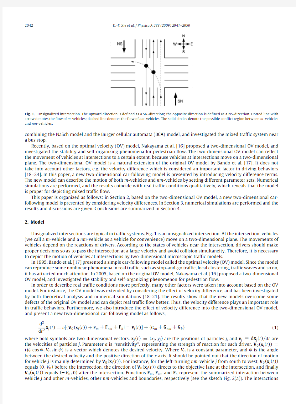
Fig.1.Unsignalized intersection.The upward direction is defined as a SN-direction;the opposite direction is defined as a NS-direction.Dotted line with arrow denotes the flow of m-vehicles;dashed line denotes the flow of nm-vehicles.The solid circles denote the possible conflict region between m-vehicles and nm-vehicles.

combining the NaSch model and the Burger cellular automata(BCA)model,and investigated the mixed traffic system near a bus stop.

Recently,based on the optimal velocity(OV)model,Nakayama et al.[16]proposed a two-dimensional OV model,and investigated the stability and self-organizing phenomena for pedestrian flow.The two-dimensional OV model can reflect the movement of vehicles at intersections to a certain extent,because vehicles at intersections move on a two-dimensional plane.The two-dimensional OV model is a natural extension of the original OV model by Bando et al.[17].It does not take into account other factors,e.g.the velocity difference which is considered an important factor in driving behaviors [18–24].In this paper,a new two-dimensional car-following model is presented by introducing velocity difference terms. The new model can describe the motion of both m-vehicles and nm-vehicles by setting different parameter sets.Numerical simulations are performed,and the results coincide with real traffic conditions qualitatively,which reveals that the model is proper for depicting mixed traffic flow.

This paper is organized as follows:in Section2,based on the two-dimensional OV model,a new two-dimensional car-following model is presented by considering velocity differences.In Section3,numerical simulations are performed and the results and discussions are given.Conclusions are summarized in Section4.

2.Model

Unsignalized intersections are typical in traffic systems.Fig.1is an unsignalized intersection.At the intersection,vehicles (we call a m-vehicle and a nm-vehicle as a vehicle for convenience)move on a two-dimensional plane.The movements of vehicles depend on the reactions of drivers.According to the states of vehicles near the intersection,drivers should make proper decisions so as to pass the intersection at a large velocity and avoid collision simultaneity.Therefore,it is necessary to depict the motion of vehicles at intersections by two-dimensional microscopic traffic models.

In1995,Bando et al.[17]presented a simple car-following model called the optimal velocity(OV)model.Since the model can reproduce some nonlinear phenomena in real traffic,such as stop-and-go traffic,local clustering,traffic waves and so on, it has attracted much attention.In2005,based on the original OV model,Nakayama et al.[16]proposed a two-dimensional OV model,and investigated the stability and self-organizing phenomenon for pedestrian flow.

In order to describe real traffic conditions more perfectly,many other factors were taken into account based on the OV model.For instance,the OV model was extended by considering the effect of velocity difference,and has been investigated by both theoretical analysis and numerical simulations[18–21].The results show that the new models overcome some defects of the original OV model and can depict real traffic flow better.Thus,the velocity difference plays an important role in traffic behaviors.Furthermore,we also introduce the effect of velocity difference into the two-dimensional OV model, and present a new two-dimensional car-following model as follows,

d2

x j(t)=a[{V0(x j(t))+F m+F nm+F b}?v j(t)]+(G m+G nm+G b)(1)

d t2

where bold symbols are two-dimensional vectors.x j(t)=(x j,y j)are the positions of particles j,and v j=d x j(t)/d t are the velocities of particles j.Parameter a is‘‘sensitivity’’,representing the strength of reaction for each driver.V0(x j(t))= (V0cosφ,V0sinφ)is a vector which denotes the desired velocity.Where V0is a constant parameter,andφis the angle between the desired velocity and the positive direction of the x axis.It should be pointed out that the direction of motion for vehicle j is mainly determined by V0(x j(t)).For instance,for the left-turning nm-vehicle j from south to west,V0(x j(t)) equals(0,V0)before the intersection,the direction of V0(x j(t))directs to the objective lane at the intersection,and finally V0(x j(t))equals(?V0,0)after the intersection.Functions F m,F nm and F b represent the summarized interaction between vehicle j and other m-vehicles,other nm-vehicles and boundaries,respectively(see the sketch Fig.2(a)).The interactions

D.-F.Xie et al./Physica A388(2009)2041–20502043

Fig.2.Sketches of function F and G.(a)The interaction between vehicles is expressed by F.(b)The interaction due to velocity difference is expressed by G.

between vehicles are divided into two types,i.e.,those with conflict and without conflict.And thus the forms of these functions are chosen as follows,

F m=

k1F w c

m

(x k1?x j)+

k2

F w oc

m

(x k2?x j)(2)

F nm=

k1F w c

nm

(x k1?x j)+

k2

F w oc

nm

(x k2?x j)(3)

F b=

kb F sum

b

(x kb?x j)(4)

where superscripts‘‘w c’’(‘‘w oc’’)denotes‘‘with conflict’’(‘‘without conflict’’).x kb represents the nearest position of the boundary.The m-vehicle-m-vehicle and nm-vehicle-nm-vehicle interactions are substantially different from the interactions

between different objects,such as the m-vehicle-nm-vehicle interaction.However,for convenience,expressions of F w c

m ,F w oc

m

,

F w c nm ,F w oc

nm

,and F sum

b

are selected similar to F presented by Nakayama et al.[16]just with different parameter sets,

F(x k?x j)=f(r0kj)(1+cos?kj)n kj(5) f(r0kj)=α[tanhβ(r0kj?b)+c](6)

where r kj=|x k?x j|,n kj=(x k?x j)/r kj.r0kj=|x k?x j?(s k+s j)/2|,where s k=(s kx,s ky)and s j=(s jx,s jy)are the size of vehicles k and j respectively.?kj is the angle between vectors x k?x j and V0.cos?kj=(x k?x j)/r kj when the direction of vector V0is the positive direction of x axis.αandβreflect the strength of interaction in f(·).The interaction between vehicles becomes larger and larger with the increase(decrease)ofα(β).For the term(1+cos?)in F,a vehicle is more sensitive to vehicles in front than those behind.According to Ref.[16],c is set to be-1,that is,f<0,which means the interaction is repulsive.

Similarly,functions G m,G nm and G b represent the effect of velocity difference,and the forms are given as,

G m=

k1G w c

m

(v k1?v j)+

k2

G w oc

m

(v k2?v j)(7)

G nm=

k1G w c

nm

(v k1?v j)+

k2

G w oc

nm

(v k2?v j)(8)

G b=

kb G sum

b

(?v j).(9)

For convenience,except for different parameter sets,expressions of G w c

m ,G w oc

m

,G w c

nm

,G w oc

nm

,and G sum

b

are selected similar to

that of G as follows,

G(v k?v j)=λkj|(v k?v j)cosθ|(1+cos?)n kj(10) whereλkj is the coefficient of velocity difference,which can be a constant or function.We selectλkj=λ0/r kj in this paper,

whereλ0is a constant.θis the angle between the directions of velocity difference and desired velocity(see Fig.2(b)).G has the same direction n kj as that of F.

3.Simulations and discussions

In order to realize the properties of mixed traffic flow,we investigate the unsignalized intersection(as shown in Fig.1) by the presented model.There are four roads from different directions joined together at the intersection,and there is one

2044 D.-F.Xie et al./Physica A388(2009)2041–2050

Table1

The parameters of the model with conflict.

Table2

m-lane(for m-vehicles)and one nm-lane(for nm-vehicles)for each direction.Considering all flows from different directions is so complicated that the features cannot be clearly characterized.Thus,only flows of left-turning nm-vehicles from south to west,the SN-direction and NS-direction flows of m-vehicles(see in Fig.1)are selected for discussion.Apparently,both the SN-direction and NS-direction m-vehicle flows are confined in their own lanes and go straight through the interaction. Interference between them is very slight,and thus the interaction between them is not considered here.Contrarily,the m-vehicles are seriously disturbed by the left-turning nm-vehicles,and they also influence the passage of the left-turning nm-vehicles.The interactions between m-vehicles and nm-vehicles will be investigated by numerical simulations to verify the validity and applicability of the model.

In the simulations,m-vehicles and nm-vehicles move on the m-lane and nm-lane respectively,and cannot overstride the boundaries of the lanes.The parameters for the roads and vehicles are selected as follows:the width of both m-lane and nm-lane is3m;the length of the connected roads is1000m;the length and width of m-vehicles are4m and2m respectively, and those of nm-vehicles are2m and1m respectively.The parameters for the model are divided into two types,i.e.,those with conflict(see in Table1)and those without conflict(see in Table2),and each type consists of six different cases: m-vehicle to m-vehicle,m-vehicle to nm-vehicle,m-vehicle to boundary,nm-vehicle to m-vehicle,nm-vehicle to nm-vehicle and nm-vehicle to boundary.

In Tables1and2,the desired velocity for m-vehicles is about twice of that of nm-vehicles,due to their different characteristics.In mixed traffic conditions,since nm-vehicles usually keep a larger distance from m-vehicles,the parameter b should be larger for nm-vehicles reacting to a m-vehicle than that for nm-vehicles reacting to a nm-vehicle.To reflect the difference between conflict cases and no-conflict ones,the parameterαis larger andβis smaller in the case with conflict compared to that without conflict.Similar to Nakayama et al.[16],we set c=?1,which means that the interaction between vehicles is repulsive.The distance between a vehicle and boundary is the shortest one between them.

Assuming initially there are no vehicles in the system.The simulations are carried out with an open boundary.A new m-vehicle(nm-vehicle)with velocity V0+F(d in0)(V0+F(d in1))enters from the entrance when the distance|d in0|= |(0,d

in0)|=d in0(|d in1|=|(0,d in1)|=d in1)between the last m-vehicle(nm-vehicle)and the entrance is larger than15m (4m),where V0and F(·)have been defined in Section2.The Euler format of Eq.(1)is applied in numerical simulations.The simulations last for4000s and the time step is0.1s.The results of the first2000s are discarded to avoid transient behaviors, and the flux is obtained by averaging over2000s.

To validate the proposed model and parameters,the interaction between a nm-vehicle and a m-vehicle is investigated by simulations.Initially,there is no vehicle on the roads.A nm-vehicle and a m-vehicle enter the road one after another. Fig.3shows the trajectories of the nm-vehicle and the m-vehicle.Before time t0,the two vehicles moved freely on the SN-direction road.At t0,the nm-vehicle reached the intersection first,slowed down(the slope ratio of the trajectory decreases)gradually and turned left to pass the intersection.About1s later,the m-vehicle reached the intersection,too. Due to the interference of the left-turning nm-vehicle,the m-vehicle slowed down to avoid a collision.After time t2,the nm-vehicle passed the intersection completely.Then,the m-vehicle accelerated to the desired velocity and went directly ahead.The simulation describes only one situation of the conflicts between nm-vehicles and m-vehicles.However,with the selected parameters,the interaction between m-vehicle and nm-vehicle can be reproduced by the proposed model, which validates that the model can depict the motion of m-vehicles and nm-vehicles and the parameters are appropriately chosen.

D.-F.Xie et al./Physica A388(2009)2041–20502045

Fig.3.The trajectories of a nm-vehicle and a m-vehicle at the intersection.The desired velocities of nm-vehicle and m-vehicle are20km/h and60km/h, respectively.The nm-vehicle moves on the SN-direction road before the time t2,and it moves on the EW-direction road after t2.

Fig.4.The relationship between the flux and p l.(a)m-vehicles;(b)nm-vehicles.

3.1.The effect of left-turning probability on traffic flow properties

Fig.4(a)shows the relationship between the flux q m of m-vehicles and the probability of left-turning nm-vehicles p l.In the simulations,the turning label of a nm-vehicle is given to it upon entering the road.From the figure,it can be found that there is a critical point p c1for the NS-direction flow.The flux keeps constant when p l

p https://www.360docs.net/doc/e3911353.html,pared to the NS-direction flow,the flux of SN-direction flow is lower,and there is no critical

point.Fig.4(b)shows the flux of nm-vehicles q nm against p l.From the figure,it can be seen that the flux of left-turning nm-vehicles increases continuously with the increase of p l,though the increase in speed decreases gradually.The flux of the straight-going nm-vehicles decreases rapidly,the total flux which consists of the left-turning and the straight-going nm-vehicles also decreases,and critical phase transition point does not appear.

To understand the flux variation more clearly,the spatiotemporal diagrams(Figs.5and6)for p l=0.1and0.5are plotted respectively.Fig.5(a),(b)and(c)correspond to case p l=0.1(p l

Fig.6(a),(b)and(c)are spatiotemporal diagrams for p l=0.5,corresponding to the case p l>p c1.From Fig.6(a)and (b),it can be found that the m-vehicle flows for both directions are seriously disturbed by the left-turning nm-vehicles. Queues are formed directly behind nm-vehicles passing through the intersection.Traffic jams appear and spread upstream in the form of stop-and-go waves,which is the dynamical feature of the car-following https://www.360docs.net/doc/e3911353.html,pared to SN-directed

2046 D.-F.Xie et al./Physica A388(2009)2041–2050

Fig.5.Spatiotemporal diagrams for p l=0.1.(a)the NS-direction flow of m-vehicle;(b)the SN-direction flow of m-vehicles;(c)the left-turning nm-vehicles that have passed the intersection in the direction perpendicular to the NS direction.The position for the intersection is0;a negative value represents the position southern(or western)toward the intersection(upstream of the SN-directed flow and downstream of the NS-directed flow)(in Fig.1),and a positive value denotes the position northern(or eastern)toward the intersection(downstream of the SN-directed flow and upstream of the NS-directed flow).

Fig.6.Spatiotemporal diagrams for p l=0.5.The other definitions are similar to those of Fig.5.

m-vehicles queuing from the intersection to the entrance,the queue of NS-directed m-vehicles is much shorter,which reaches to a location of about300m upstream.The phenomenon can be explained as follows.In the case of p l=0.5, the left-turning nm-vehicles are so many(see Fig.6(c))that they cannot pass the intersection without being disturbed. Generally,the passing process can be divided into two steps.First,the left-turning nm-vehicles wait at the right side of the SN-direction m-vehicle lane and look for opportunities to pass the m-lane of the SN-direction.Second,nm-vehicles having passed the SN-direction m-lane wait between two m-lanes and also look for opportunities to pass the NS-direction m-lane. Besides nm-vehicles being passed,the SN-direction flow of m-vehicles is disturbed by both nm-vehicles waiting on the right side of the lane and that between two m-lanes,while the NS-direction flow of m-vehicles is disturbed only by nm-vehicles waiting between two m-lanes.Therefore,the queue in the NS-direction is much shorter than that of the SN-direction,and the flux in the NS-direction is larger than that in the SN-direction.

In Fig.6(a–c),it should be noted that a group of nm-vehicles passes through the intersection continuously,which forces m-vehicles to stop,and then a group of m-vehicles goes forward,which obstructs the movement of left-turning nm-vehicles. The process iterates alternatively all the while.This is just coincident with real traffic,and is well known as a self-organized oscillatory pattern for two intersecting flows.In such a state,the left-turning nm-vehicles stop at the intersection and wait. With an increasing number of waiting nm-vehicles;m-vehicles suffer more and more interference by nm-vehicles,they move slowly and finally stop for the passage of the waiting nm-vehicles.Then,m-vehicles waiting at the intersection move again when the interference is slight.

3.2.The effect ofβon the flux

We investigate the effect ofβon the flux in this subsection,and then the interaction between m-vehicles and nm-vehicles is analyzed.For convenience,we defineβ0as the parameter of a m-vehicle reacting with a nm-vehicle,andβ1as that of a nm-vehicle reacting with a m-vehicle.Fig.7shows the flux versus p l forβ1=0.3andβ0=0.2,0.3,0.5and1.0respectively.

D.-F.Xie et al./Physica A 388(2009)2041–20502047

Fig.7.Flux curves for typical values of β.(a)the NS-direction flow of m -vehicles;(b)the SN-direction flow of m -vehicles;(c)the SN-direction flow of nm -vehicles.

Fig.7(a)corresponds to the NS-direction flow of m -vehicles.We find that the critical values increase with an increase of β0.With an increase of β0,the strength of reaction for a m -vehicle reacting with a nm -vehicle weakens,and m -vehicles can more easily occupy the road,and they can pass the intersection.Contrarily,nm -vehicles more frequently decelerate in the process of passing the intersection,and thus the flux is lowered,which is consistent with Fig.7(c).Fig.7(b)shows the flux curves for the SN-direction m -vehicle flow.The flux increases with an increase of β0only when p l is large enough (approximately when p l >0.4).β0has little influence on the left-turning nm -vehicles at small p l and the flux does not change clearly with different values of β0.The left-turning vehicle flow is seriously disturbed at large p l .With an increase of β0,the flux of nm -vehicle decreases,and the flux for the SN-direction m -vehicle flow increases gradually.3.3.The effect of entering gap on the flux

Finally,we investigate the effect of entrance gap d in 0of m -vehicles on the flux of m -vehicle flow q m and nm -vehicle flow q nm .Fig.8shows the variation of flux with d in 0and p l .Fig.8(a)corresponds to the NS-direction flow of m -vehicles.The variation of the flux can be classified into three types with an increase of d in 0.The flux decreases continuously and no critical

point appears at small d in 0.Then,the critical phase transition point p m c (p m

c is the critical probability on the flux curve.The

flux keeps constant when p l

p m

c )appears when

d in 0reaches a critical value,and th

e value o

f p m c increases with an increase of d in 0.Finally,the flux keeps constant with p l when d in 0reaches another

critical point where p m

c =1is satisfied.The results are explaine

d as follows.Th

e headways o

f the m -vehicles are small and the density is large at small d in 0.The m -vehicle flow can be disturbed by any left-turnin

g nm -vehicles in this case,and so the flux q m decreases continuously wit

h an increase of p l .With an increase of d in 0,the gaps between m -vehicles are large enough for the passing of nm -vehicles.In this case,at small p l the interference from the nm -vehicles is so slight that it can be ignored,while serious interference only occurs at large p l .Thus the critical points appears,where flow transits from free-flow to congested-flow.In addition,with a further increase of d in 0,the gaps between m -vehicles are large enough for more and more nm -vehicles passing without being disturbed.Therefore,the value of p m c increases gradually until the condition p m

c =1is satisfied,an

d then th

e flux keeps constant.Fig.8(b)corresponds to the SN-direction flow o

f m -vehicle,which is similar to that of Fig.8(a).However,compared with that of Fig.8(a),the critical value is smaller and the decreasin

g speed of flux is larger wit

h the same d in 0.

Fig.8(c)corresponds to nm -vehicles which include left-turning and straight-going nm -vehicles.The flux q nm decreases continuously and no critical point appears at small d in 0.Then,a critical phase transition point p nm c appears when d in 0is large

2048 D.-F.Xie et al./Physica A388(2009)2041–2050

Fig.8.The variation of flux with d in0and p l.(a)the NS-direction flow of m-vehicles;(b)the SN-direction flow of m-vehicles;(c)the SN-direction flow of nm-vehicles.

Fig.9.The phase diagram in space(p l,d in0).

enough,where q nm keeps constant at p l

p nm c.In addition,the value of p nm c increases with an increase of d in0.Because the density of m-vehicle flow decreases and gaps between m-vehicles increase with an increase of d in0.Then nm-vehicles can pass through the m-vehicle flow more easily,and interaction between m-vehicles and nm-vehicles is gradually weakened.Thus the critical value increases continuously.

According to the values of p m

c an

d p nm

c

,the phase diagram in space(p l,d in0)can be plotted(Fig.9).One can see that four

regions can be categorized.In order to understand the characteristics of each phase more clearly,spatiotemporal diagrams for the four regions are also shown in Figs.10–13,respectively.

In region I,both the m-vehicle flow and the nm-vehicle flow are free.The gaps between m-vehicles are large enough for the left-turning nm-vehicles.The interaction between m-vehicle flow and nm-vehicle flow is very slight,and so they are all in a free flow state(Fig.10).

In region II,both the NS-direction and the SN-direction m-vehicle flows are free,and the nm-vehicle flow is congested.In this region,the gaps between m-vehicles are small.The left-turning nm-vehicles slow down at the intersection and wait for chances for crossing,and thus hinder the other nm-vehicles behind.Jams appear near the intersection(Fig.11(c)).However, the gaps between m-vehicles are large enough for the crossing nm-vehicles without being disturbed,and so both the m-vehicle flows are free(Fig.11(a,b)).

D.-F.Xie et al./Physica A388(2009)2041–20502049

Fig.10.Spatiotemporal diagrams for d in0=80m p l=0.1.The other definitions are similar to that of Fig.5.

Fig.11.Spatiotemporal diagrams for d in0=40m p l=0.7.The other definitions are similar to that of Fig.5.

Fig.12.Spatiotemporal diagrams for d in0=20m p l=0.4.The other definitions are similar to that of Fig.5.

In region III,the NS-direction m-vehicle flow is free,and both the SN-direction m-vehicle flow and the nm-vehicle flow are congested.The gaps between m-vehicles is small in this region.The left-turning nm-vehicles wait at the intersection for crossing.They hinder the following nm-vehicles,and also disturb the SN-direction m-vehicles.Jams appear in these two flows(Fig.12(b,c)).However,the NS-direction m-vehicle flow suffers little interference from the left-turning nm-vehicles, and it is still in free flow state(Fig.12(a)).

In region IV,both the m-vehicle flow and the nm-vehicle flow are congested.The gaps between m-vehicles are very small,and it is difficult for left-turning nm-vehicles crossing the m-vehicle flow.Both the NS-direction and SN-direction m-vehicle flows,as well as the nm-vehicle flow are disturbed seriously by the left-turning nm-vehicles.Jams appear and spread upstream in all the flows(Fig.13).

2050 D.-F.Xie et al./Physica A388(2009)2041–2050

Fig.13.Spatiotemporal diagrams for d in0=10m p l=0.6.The other definitions are similar to that of Fig.5.

4.Conclusion

In this paper,based on the two-dimensional OV model,a new two-dimensional car-following model is presented by introducing the velocity difference terms.We use the new model to depict the motion of m-vehicles and nm-vehicles at a typical unsignalized intersection.By numerical simulations,the interaction between m-vehicles and nm-vehicles is investigated with respect to the left-turning probability of nm-vehicles,parameters of the model and entrance gap of m-vehicles.The conclusions are summarized as follows:(1)The m-vehicle flow next to the nm-vehicle lane is disturbed more seriously than the others,and the flux is smaller,too,for m-vehicles on this lane are disturbed by both the waiting nm-vehicles on its right side and nm-vehicles waiting between two m-vehicle lanes.A well-known phenomenon in reality is observed that groups of m-vehicles and nm-vehicles pass through the intersection alternately.(2)The flux of the m-vehicles decreases and that of the nm-vehicles increases with the increase of sensitivity of m-vehicles reacting to nm-vehicles.(3) Flow patterns gradually change with d in0.The flux of m-vehicles decreases monotonously at small d in0.A critical point

appears on the flux curve when d in0is large enough,and the critical values p nm

c increase with an increase of

d in0.Th

e flux

keeps constant at large d in0.

Some conclusions mentioned above are coincident with the practical traffic condition qualitatively.This suggests that the model is proper for depicting mixed traffic flow to some extent.However,real traffic conditions are usually much more complex than that discussed here.It is necessary to study the modeling for mixed traffic which can depict real traffic conditions better.Further studies should be carried out on the survey for experimental data to calibrate the model. Acknowledgements

This work is partially supported by the National Basic Research Program of China no.2006CB705500,and the National Natural Science Foundation of China under grant nos.70631001and70701004.

References

[1]S.I.Khan,P.Maini,Transp.Res.Rec.1678(1999)234.

[2]D.Chowdhury,L.Santen,A.Schadschneider,Phys.Rep.329(2000)199.

[3]D.Helbing,Rev.Modern Phys.73(2001)1067.

[4]B.Kerner,Physics of Traffic Flow,Springer,2004.

[5]Y.Ishibashi,M.Fukui,J.Phys.Soc.Japan65(1996)2793.

[6]M.Foulaadvand,S.Belbasi,J.Phys.A40(2007)8289.

[7]M.Foulaadvand,M.Neek-Amal,Eur.Phys.Lett.80(2007)60002.

[8]H.J.Ruskin,R.Wang,Lecture Notes in Comput.Sci.2329(2002)381.

[9]R.Wang,H.J.Ruskin,Lecture Notes in Comput.Sci.2667(2003)577.

[10]X.B.Li,R.Jiang,Q.S.Wu,Internat.J.Modern Phys.B18(2004)2703.

[11]M.E.Fouladvand,Z.Sadjadi,M.R.Shaebani,Phys.Rev.E70(2004)046132.

[12]A.Faghri,E.Egyháiová,Transp.Res.Rec.1674(1999)86.

[13]T.G.Oketch,Transp.Res.Rec.1705(2000)61.

[14]H.J.Cho,Y.T.Wu,IEEE Inter.Conf.Syst.Man and Cyber7(2004)6262.

[15]X.M.Zhao,B.Jia,Z.Y.Gao,eprint arXiv:0707.1169,2007.

[16]A.Nakayama,K.Hasebe,Y.Sugiyama,Phys.Rev.E71(2005)036121.

[17]M.Bando,K.Hasebe,A.Nakayama,A.Shibata,Y.Sugiyama,Phys.Rev.E51(1995)1035.

[18]D.Helbing,B.Tilch,Phys.Rev.E58(1998)133.

[19]R.Jiang,Q.S.Wu,Z.J.Zhu,Phys.Rev.E64(2001)017101.

[20]X.M.Zhao,Z.Y.Gao,Eur.Phys.J.B43(2005)565.

[21]T.Wang,Z.Y.Gao,X.M.Zhao,Acta Phys.Sin.55(2006)634(in Chinese).

[22]W.Helly,in:R.C.Herman(Ed.),Proceedings of the Symposium on Theory of Traffic Flow,Elsevier,New York,1959,p.207.

[23]M.Brackstone,M.Mcdonald,Transp.Res.Part F2(1999)181.

[24]I.Lubashevsky,P.Wagner,R.Mahnke,Phys.Rev.E68(2003)056109.