6PH02_01_que_20100609 Edexcel GCE Physics

合集下载

高质量DXT压缩使用CUDA技术（2009年）说明书

March 2009High Quality DXT Compression using OpenCL for CUDAIgnacio Castaño*******************Document Change HistoryVersion Date Responsible Reason for Change0.1 02/01/2007 Ignacio Castaño First draft0.2 19/03/2009 Timo Stich OpenCL versionAbstractDXT is a fixed ratio compression format designed for real-time hardware decompression of textures. While it’s also possible to encode DXT textures in real-time, the quality of the resulting images is far from the optimal. In this white paper we will overview a more expensivecompression algorithm that produces high quality results and we will see how to implement it using CUDA to obtain much higher performance than the equivalent CPU implementation.MotivationWith the increasing number of assets and texture size in recent games, the time required to process those assets is growing dramatically. DXT texture compression takes a large portion of this time. High quality DXT compression algorithms are very expensive and while there are faster alternatives [1][9], the resulting quality of those simplified methods is not very high. The brute force nature of these compression algorithms makes them suitable to be parallelized and adapted to the GPU. Cheaper compression algorithms have already been implemented [2] on the GPU using traditional GPGPU approaches. However, with the traditional GPGPU programming model it’s not possible to implement more complex algorithms where threads need to share data and synchronize.How Does It Work?In this paper we will see how to use CUDA to implement a high quality DXT1 texturecompression algorithm in parallel. The algorithm that we have chosen is the cluster fit algorithm as described by Simon Brown [3]. We will first provide a brief overview of the algorithm and then we will describe how did we parallelize and implement it in CUDA.DXT1 FormatDXT1 is a fixed ratio compression scheme that partitions the image into 4x4 blocks. Each block is encoded with two 16 bit colors in RGB 5-6-5 format and a 4x4 bitmap with 2 bits per pixel. Figure 1 shows the layout of the block.Figure 1. DXT1 block layoutThe block colors are reconstructed by interpolating one or two additional colors between the given ones and indexing these and the original colors with the bitmap bits. The number of interpolated colors is chosen depending on whether the value of ‘Color 0’ is lower or greater than ‘Color 1’.BitmapColorsThe total size of the block is 64 bits. That means that this scheme achieves a 6:1 compression ratio. For more details on the DXT1 format see the specification of the OpenGL S3TCextension [4].Cluster FitIn general, finding the best two points that minimize the error of a DXT encoded block is a highly discontinuous optimization problem. However, if we assume that the indices of the block are known the problem becomes a linear optimization problem instead: minimize the distance from each color of the block to the corresponding color of the palette.Unfortunately, the indices are not known in advance. We would have to test them all to find the best solution. Simon Brown [3] suggested pruning the search space by considering only the indices that preserve the order of the points along the least squares line.Doing that allows us to reduce the number of indices for which we have to optimize theendpoints. Simon Brown provided a library [5] that implements this algorithm. We use thislibrary as a reference to compare the correctness and performance of our CUDAimplementation.The next section goes over the implementation details.OpenCL ImplementationPartitioning the ProblemWe have chosen to use a single work group to compress each 4x4 color block. Work items that process a single block need to cooperate with each other, but DXT blocks are independent and do not need synchronization or communication. For this reason the number of workgroups is equal to the number of blocks in the image.We also parameterize the problem so that we can change the number of work items per block to determine what configuration provides better performance. For now, we will just say that the number of work items is N and later we will discuss what the best configuration is.During the first part of the algorithm, only 16 work items out of N are active. These work items start reading the input colors and loading them to local memory.Finding the best fit lineTo find a line that best approximates a set of points is a well known regression problem. The colors of the block form a cloud of points in 3D space. This can be solved by computing the largest eigenvector of the covariance matrix. This vector gives us the direction of the line.Each element of the covariance matrix is just the sum of the products of different colorcomponents. We implement these sums using parallel reductions.Once we have the covariance matrix we just need to compute its first eigenvector. We haven’t found an efficient way of doing this step in parallel. Instead, we use a very cheap sequential method that doesn’t add much to the overall execution time of the group.Since we only need the dominant eigenvector, we can compute it directly using the Power Method [6]. This method is an iterative method that returns the largest eigenvector and only requires a single matrix vector product per iteration. Our tests indicate that in most cases 8iterations are more than enough to obtain an accurate result.Once we have the direction of the best fit line we project the colors onto it and sort them along the line using brute force parallel sort. This is achieved by comparing all the elements against each other as follows:cmp[tid] = (values[0] < values[tid]);cmp[tid] += (values[1] < values[tid]);cmp[tid] += (values[2] < values[tid]);cmp[tid] += (values[3] < values[tid]);cmp[tid] += (values[4] < values[tid]);cmp[tid] += (values[5] < values[tid]);cmp[tid] += (values[6] < values[tid]);cmp[tid] += (values[7] < values[tid]);cmp[tid] += (values[8] < values[tid]);cmp[tid] += (values[9] < values[tid]);cmp[tid] += (values[10] < values[tid]);cmp[tid] += (values[11] < values[tid]);cmp[tid] += (values[12] < values[tid]);cmp[tid] += (values[13] < values[tid]);cmp[tid] += (values[14] < values[tid]);cmp[tid] += (values[15] < values[tid]);The result of this search is an index array that references the sorted values. However, this algorithm has a flaw, if two colors are equal or are projected to the same location of the line, the indices of these two colors will end up with the same value. We solve this problem comparing all the indices against each other and incrementing one of them if they are equal:if (tid > 0 && cmp[tid] == cmp[0]) ++cmp[tid];if (tid > 1 && cmp[tid] == cmp[1]) ++cmp[tid];if (tid > 2 && cmp[tid] == cmp[2]) ++cmp[tid];if (tid > 3 && cmp[tid] == cmp[3]) ++cmp[tid];if (tid > 4 && cmp[tid] == cmp[4]) ++cmp[tid];if (tid > 5 && cmp[tid] == cmp[5]) ++cmp[tid];if (tid > 6 && cmp[tid] == cmp[6]) ++cmp[tid];if (tid > 7 && cmp[tid] == cmp[7]) ++cmp[tid];if (tid > 8 && cmp[tid] == cmp[8]) ++cmp[tid];if (tid > 9 && cmp[tid] == cmp[9]) ++cmp[tid];if (tid > 10 && cmp[tid] == cmp[10]) ++cmp[tid];if (tid > 11 && cmp[tid] == cmp[11]) ++cmp[tid];if (tid > 12 && cmp[tid] == cmp[12]) ++cmp[tid];if (tid > 13 && cmp[tid] == cmp[13]) ++cmp[tid];if (tid > 14 && cmp[tid] == cmp[14]) ++cmp[tid];During all these steps only 16 work items are being used. For this reason, it’s not necessary to synchronize them. All computations are done in parallel and at the same time step, because 16 is less than the warp size on NVIDIA GPUs.Index evaluationAll the possible ways in which colors can be clustered while preserving the order on the line are known in advance and for each clustering there’s a corresponding index. For 4 clusters there are 975 indices that need to be tested, while for 3 clusters there are only 151. We pre-compute these indices and store them in global memory.We have to test all these indices and determine which one produces the lowest error. In general there are indices than work items. So, we partition the total number of indices by the number of work items and each work item loops over the set of indices assigned to it. It’s tempting to store the indices in constant memory, but since indices are used only once for each work group, and since each work item accesses a different element, coalesced global memory loads perform better than constant loads.Solving the Least Squares ProblemFor each index we have to solve an optimization problem. We have to find the two end points that produce the lowest error. For each input color we know what index it’s assigned to it, so we have 16 equations like this:i i i x b a =+βαWhere {}i i βα, are {}0,1, {}32,31, {}21,21, {}31,32 or {}1,0 depending on the index and the interpolation mode. We look for the colors a and b that minimize the least square error of these equations. The solution of that least squares problem is the following:∑∑⋅∑∑∑∑= −i i i i i ii i i i x x b a βαββαβαα122 Note: The matrix inverse is constant for each index set, but it’s cheaper to compute it everytime on the kernel than to load it from global memory. That’s not the case of the CPU implementation.Computing the ErrorOnce we have a potential solution we have to compute its error. However, colors aren’t stored with full precision in the DXT block, so we have to quantize them to 5-6-5 to estimate the error accurately. In addition to that, we also have to take in mind that the hardware expands thequantized color components to 8 bits replicating the highest bits on the lower part of the byte as follows:R = (R << 3) | (R >> 2); G = (G << 2) | (G >> 4); B = (B << 3) | (B >> 2);Converting the floating point colors to integers, clamping, bit expanding and converting them back to float can be time consuming. Instead of that, we clamp the color components, round the floats to integers and approximate the bit expansion using a multiplication. We found the factors that produce the lowest error using an offline optimization that minimized the average error.r = round(clamp(r,0.0f,1.0f) * 31.0f); g = round(clamp(g,0.0f,1.0f) * 63.0f); b = round(clamp(b,0.0f,1.0f) * 31.0f); r *= 0.03227752766457f; g *= 0.01583151765563f; b *= 0.03227752766457f;Our experiment show that in most cases the approximation produces the same solution as the accurate solution.Selecting the Best SolutionFinally, each work item has evaluated the error of a few indices and has a candidate solution.To determine which work item has the solution that produces the lowest error, we store the errors in local memory and use a parallel reduction to find the minimum. The winning work item writes the endpoints and indices of the DXT block back to global memory.Implementation DetailsThe source code is divided into the following files:•DXTCompression.cl: This file contains OpenCL implementation of the algorithm described here.•permutations.h: This file contains the code used to precompute the indices.dds.h: This file contains the DDS file header definition. PerformanceWe have measured the performance of the algorithm on different GPUs and CPUscompressing the standard Lena. The design of the algorithm makes it insensitive to the actual content of the image. So, the performance depends only on the size of the image.Figure 2. Standard picture used for our tests.As shown in Table 1, the GPU compressor is at least 10x faster than our best CPUimplementation. The version of the compressor that runs on the CPU uses a SSE2 optimized implementation of the cluster fit algorithm. This implementation pre-computes the factors that are necessary to solve the least squares problem, while the GPU implementation computes them on the fly. Without this CPU optimization the difference between the CPU and GPU version is even larger.Table 1. Performance ResultsImage TeslaC1060 Geforce8800 GTXIntel Core 2X6800AMD Athlon64 DualCore 4400Lena512x51283.35 ms 208.69 ms 563.0 ms 1,251.0 msWe also experimented with different number of work-items, and as indicated in Table 2 we found out that it performed better with the minimum number.Table 2. Number of Work Items64 128 25654.66 ms 86.39 ms 96.13 msThe reason why the algorithm runs faster with a low number of work items is because during the first and last sections of the code only a small subset of work items is active.A future improvement would be to reorganize the code to eliminate or minimize these stagesof the algorithm. This could be achieved by loading multiple color blocks and processing them in parallel inside of the same work group.ConclusionWe have shown how it is possible to use OpenCL to implement an existing CPU algorithm in parallel to run on the GPU, and obtain an order of magnitude performance improvement. We hope this will encourage developers to attempt to accelerate other computationally-intensive offline processing using the GPU.High Quality DXT Compression using CUDAMarch 2009 9References[1] “Real-Time DXT Compression”, J.M.P. van Waveren. /cd/ids/developer/asmo-na/eng/324337.htm[2] “Compressing Dynamically Generated Textures on the GPU”, Oskar Alexandersson, Christoffer Gurell, Tomas Akenine-Möller. http://graphics.cs.lth.se/research/papers/gputc2006/[3] “DXT Compression Techniques”, Simon Brown. /?article=dxt[4] “OpenGL S3TC extension spec”, Pat Brown. /registry/specs/EXT/texture_compression_s3tc.txt[5] “Squish – DXT Compression Library”, Simon Brown. /?code=squish[6] “Eigenvalues and Eigenvectors”, Dr. E. Garcia. /information-retrieval-tutorial/matrix-tutorial-3-eigenvalues-eigenvectors.html[7] “An Experimental Analysis of Parallel Sorting Algorithms”, Guy E. Blelloch, C. Greg Plaxton, Charles E. Leiserson, Stephen J. Smith /blelloch98experimental.html[8] “NVIDIA CUDA Compute Unified Device Architecture Programming Guide”.[9] NVIDIA OpenGL SDK 10 “Compress DXT” sample /SDK/10/opengl/samples.html#compress_DXTNVIDIA Corporation2701 San Tomas ExpresswaySanta Clara, CA 95050 NoticeALL NVIDIA DESIGN SPECIFICATIONS, REFERENCE BOARDS, FILES, DRAWINGS, DIAGNOSTICS, LISTS, AND OTHER DOCUMENTS (TOGETHER AND SEPARATELY, “MATERIALS”) ARE BEING PROVIDED “AS IS.” NVIDIA MAKES NO WARRANTIES, EXPRESSED, IMPLIED, STATUTORY, OR OTHERWISE WITH RESPECT TO THE MATERIALS, AND EXPRESSLY DISCLAIMS ALL IMPLIED WARRANTIES OF NONINFRINGEMENT,MERCHANTABILITY, AND FITNESS FOR A PARTICULAR PURPOSE.Information furnished is believed to be accurate and reliable. However, NVIDIA Corporation assumes no responsibility for the consequences of use of such information or for any infringement of patents or otherrights of third parties that may result from its use. No license is granted by implication or otherwise under any patent or patent rights of NVIDIA Corporation. Specifications mentioned in this publication are subject to change without notice. This publication supersedes and replaces all information previously supplied. NVIDIA Corporation products are not authorized for use as critical components in life support devices or systems without express written approval of NVIDIA Corporation.TrademarksNVIDIA, the NVIDIA logo, GeForce, and NVIDIA Quadro are trademarks or registeredtrademarks of NVIDIA Corporation in the United States and other countries. Other company and product names may be trademarks of the respective companies with which they are associated. Copyright© 2009 NVIDIA Corporation. All rights reserved.。

office各版本下载地址

2021.3最新office2010激活码推荐附激活工具+激活教程

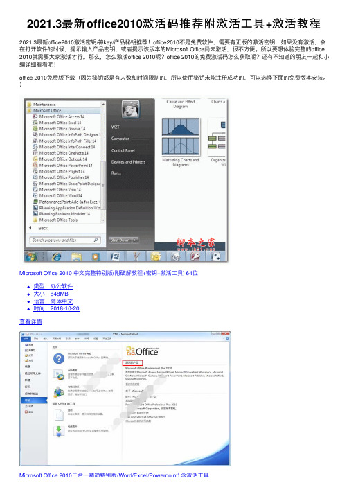
2021.3最新office2010激活码推荐附激活⼯具+激活教程2021.3最新office2010激活密钥/神key/产品秘钥推荐！office2010不是免费软件，需要有正版的激活密钥，如果没有激活，会在打开软件的时候，提⽰输⼊产品密钥，或者提⽰该版本的Microsoft Office尚未激活，很不⽅便。

所以要想体验完整的office 2010就需要⼤家激活才⾏。

那么，怎么激活office 2010呢？office 2010的免费激活码怎么获取呢？还有不知道的朋友⼀起和⼩编详细看看吧！office 2010免费版下载（因为秘钥都是有⼈数和时间限制的，所以使⽤秘钥未能注册成功的，可以选择下⾯的免费版本安装。

）Microsoft Office 2010 中⽂完整特别版(附破解教程+密钥+激活⼯具) 64位类型：办公软件⼤⼩：848MB语⾔：简体中⽂时间：2018-10-20查看详情Microsoft Office 2010三合⼀精简特别版(Word/Excel/Powerpoint) 含激活⼯具Microsoft Office 2010三合⼀精简特别版(Word/Excel/Powerpoint) 含激活⼯具类型：办公软件⼤⼩：97.8MB语⾔：简体中⽂时间：2017-12-15查看详情Macabacus for Microsoft Office2010/2013/2016 v8.11.8 特别版(附注册⽂件)类型：办公软件⼤⼩：47MB语⾔：简体中⽂时间：2019-04-26查看详情office永久数字通⽤激活⼯具HEU KMS Activator激活⼯具(⽀持win11永久激活) v24.5.0 知彼⽽知⼰版类型：系统其它⼤⼩：7.27MB语⾔：简体中⽂时间：2021-11-19查看详情KMS Matrix(windows/office⼀键激活⼯具) v4.1 免费绿⾊版类型：系统其它⼤⼩：9.7MB语⾔：英⽂软件时间：2020-11-18查看详情2021最新office2010激活密钥BDD3G-XM7FB-BD2HM-YK63V-VQFDKVYBBJ-TRJPB-QFQRF-QFT4D-H3GVBHQ937-PP69X-8K3KR-VYY2F-RPHB3MKCGC-FBXRX-BMJX6-F3Q8C-2QC6PD83RR-G22Y6-WYPTV-MG4TJ-MGH3Q236TW-X778T-8MV9F-937GT-QVKBB87VT2-FY2XW-F7K39-W3T8R-XMFGFQY89T-88PV8-FD7H7-CJVCQ-GJ49223TGP-FTKV6-HTHGD-PDWWP-MWCRQGDQ98-KW37Y-MVR84-246FH-3T6BG6VCWT-QBQVD-HG7KD-8BW8C-PBX7T7TRBP-9YRB2-QMTMW-GTGQC-7VPVFQ2CQ6-KPH24-CJ2WV-3HHH6-G2D3XPXMWD-YCJ8H-R3MXR-JJWFP-CKF7TVYBBJ-TRJPB-QFQRF-QFT4D-H3GVB7X9XM-HGMB4-TMGHY-9VDQV-R8CGBHV7BJ-R6GCT-VHBXD-YH4FD-GTH2TGFBFM-BX4DR-CK6PM-FY8YF-KBXFV4F3B6-JTT3F-VDCD6-G7J4Q-74W3R2MHJR-V4MR2-V4W2Y-72MQ7-KC6XKOffice2010永久激活密钥：7X9XM-HGMB4-TMGHY-9VDQV-R8CGBHV7BJ-R6GCT-VHBXD-YH4FD-GTH2TVYBBJ-TRJPB-QFQRF-QFT4D-H3GVBJ33GT-XVVYK-VHBBC-VY7FB-MTQ4CGRPWH-7CDHQ-K3G3C-JH2KX-C88H86CCCX-Y93YP-3WQGT-YCKFW-QTTT76QFDX-PYH2G-PPYFD-C7RJM-BBKQ8BDD3G-XM7FB-BD2HM-YK63V-VQFDKVYBBJ-TRJPB-QFQRF-QFT4D-H3GVBDBXYD-TF477-46YM4-W74MH-6YDQ8Office 2010 Professional Plus Retail(零售版)密钥key: C6YV2-6CKK8-VF7JB-JJCFM-HXJ2DGCXQJ-KFYBG-XR77F-XF3K8-WT7QW23TGP-FTKV6-HTHGD-PDWWP-MWCRQQY89T-88PV8-FD7H7-CJVCQ-GJ492GDQ98-KW37Y-MVR84-246FH-3T6BGFGVT2-GBV2M-YG4BD-JM823-XJYRYTTWC8-Y8KD3-YD77J-RGWTF-DTG2VOffice home and student 2010：HV7BJ-R6GCT-VHBXD-YH4FD-GTH2Toffice 2010 专业版密钥:NW8E5-P49TH-1GVJN-554PL-LGJJAVJ5ID-K6NEX-10583-8Z9QU-PJB1OX0JPA-CUSBK-T0J8O-2IH6W-DT6N1Office Professional Plus 2010 密钥：J33GT-XVVYK-VHBBC-VY7FB-MTQ4CGRPWH-7CDHQ-K3G3C-JH2KX-C88H86CCCX-Y93YP-3WQGT-YCKFW-QTTT76QFDX-PYH2G-PPYFD-C7RJM-BBKQ8BDD3G-XM7FB-BD2HM-YK63V-VQFDKVYBBJ-TRJPB-QFQRF-QFT4D-H3GVBDBXYD-TF477-46YM4-W74MH-6YDQ8想要获取更多资源请扫码关注公众号后台回复“649”获取激活⼯具office 2010激活教程打开刚安装的Office，点击左上⾓的“⽂件”，然后点击下拉菜单中“帮助”，显⽰为该Office需要激活。

CydXisasubunitof...

copper centers(Cu A and Cu B)and two hemes—low-spin heme a and high-spin heme a3.Despite many years of research,the individual absolute absorption spectra of the two hemes in the Soret band(420–460nm)have not yet been resolved because they overlap strongly. There is but a single classical work of Vanneste[1]reporting the absolute individual spectra of the reduced hemes a and a3.We revisited the problem with new approaches as summarized below.(1)Calcium binding to mitochondrial COX induces a small red shift of the absorption spectrum of heme a.Treating the calcium-induced difference spectrum as theﬁrst derivative(differential)of the ab-sorption spectrum of the reduced heme a,it is possible to reconstruct the line shape of the parent absolute spectrum of a2+by integration. The Soret band absolute spectrum of the reduced heme a obtained in this way differs strongly form that in ref.[1].It is fairly symmetric and can be easily approximated by two10nm Gaussians with widely split maxima at442and451nm.In contrast to Vanneste,no evidence for the~428nm shoulder is observed for heme a2+.(2)The overall Soret band of the reduced COX reveals at least5 more Gaussians that are not affected by Ca2+.Two of them at436 and443nm can be attributed to electronic B0transitions in heme a3, and two more can represent their vibronic satellites.(3)A theoretical dipole–dipole interaction model was developed [2]for calculation of absorption and CD spectra.The model allows to optimize parameters of the B x,y electronic transitions in the hemes a and a3to obtain bestﬁt to the experimental spectra.The optimized parameters agree with the characteristics of the reconstructed spectra of hemes a and a3.References[1]W.H.Vanneste,The stoichiometry and absorption spectra ofcomponents a and a-3in cytochrome c oxidase,Biochemistry,5 (1966)838–48.[2]A.V.Dyuba,A.M.Arutyunyan,T.V.Vygodina,N.V.Azarkina,A.V.Kalinovich,Y.A.Sharonov,and A.A.Konstantinov,Circular dichroism of cytochrome c oxidase,Metallomics,3(2011),417–432.doi:10.1016/j.bbabio.2014.05.171S9.P8Flavodiiron enzymes as oxygen and/or nitric oxide reductases Vera Gonçalves a,b,João B.Vicente b,c,Liliana Pinto a,Célia V.Romão a, Carlos Frazão a,Paolo Sarti d,e,f,Alessandro Giuffrèf,Miguel Teixeira a a Instituto de Tecnologia Química e Biológica António Xavier,Universidade Nova de Lisboa,Av.da República,2781–901Oeiras,Portugalb Metabolism and Genetics Group,Institute for Medicines and Pharmaceutical Sciences(iMed.UL),Faculty of Pharmacy,University of Lisbon,Av.Prof.Gama Pinto,1649–003Lisboa,Portugalc Department of Biochemistry and Human Biology,Faculty of Pharmacy, University of Lisbon,Av.Prof.Gama Pinto,1649-003Lisboa,Portugald Department of Biochemical Sciences,Sapienza University of Rome,Piazzale Aldo Moro5,I-00185Rome,Italye Fondazione Cenci Bolognetti—Istituto Pasteur,Italyf Institute of Biology,Molecular Medicine and Nanobiotechnology,National Research Council of Italy(CNR),ItalyE-mail:**************.ptThe Flavodiiron proteins(FDPs)are present in all life domains, from unicellular microbes to higher eukaryotes.FDPs reduce oxygen to water and/or nitrous oxide to nitrous oxide,actively contributing to combat the toxicity of O2or NO.The catalytic ability of FDPs is comparable to that of bonaﬁde heme–copper/iron O2/NO transmem-brane reductases.FDPs are multi-modular water soluble enzymes, exhibiting a two-domain catalytic core,whose the minimal functional unit is a‘head-to-tail’homodimer,each monomer being built by a beta-lactamase domain harbouring a diiron catalytic site,and a short-chainﬂavodoxin,binding FMN[1–3].Despite extensive data collected on FDPs,the molecular determi-nants deﬁning their substrate selectivity remain unclear.To clarify this issue,two FDPs with known and opposite substrate preferences were analysed and compared:the O2-reducing FDP from the eukaryote Entamoeba histolytica(EhFdp1)and the NO reductase FlRd from Escherichia coli.While the metal ligands are strictly conserved in these two enzymes,differences near the active site were observed.Single and double mutants of the EhFdp1were produced by replacing the residues in these positions with their equivalent in the E.coli FlRd.The biochemical and biophysical features of the EhFdp1WT and mutants were studied by potentiometric-coupled spectroscopic methods(UV–visible and EPR spectroscopies).The O2/NO reactivity was analysed by amperometric methods and stopped-ﬂow absorption spectroscopy.The reactivity of the mutants towards O2was negatively affected, while their reactivity with NO was enhanced.These observations suggest that the residues mutated have a role in deﬁning the substrate selectivity and reaction mechanism.References[1]C.Frazao,G.Silva,C.M.Gomes,P.Matias,R.Coelho,L.Sieker,S.Macedo,M.Y.Liu,S.Oliveira,M.Teixeira,A.V.Xavier,C.Rodrigues-Pousada,M.A.Carrondo,J.Le Gall,Structure of a dioxygen reduction enzyme from Desulfovibrio gigas,Nature Structural Biology,7(2000)1041–1045.[2]J.B.Vicente,M.A.Carrondo,M.Teixeira,C.Frazão,FlavodiironProteins:Nitric Oxide and/or Oxygen Reductases,in:Encyclopedia of Inorganic and Bioinorganic Chemistry,(2011).[3]V.L.Gonçalves,J.B.Vicente,L.M.Saraiva,M.Teixeira,FlavodiironProteins and their role in cyanobacteria,in: C.Obinger,G.A.Peschek(Eds.)Bioenergetic Processes of Cyanobacteria,Springer Verlag,(2011),pp.631–656.doi:10.1016/j.bbabio.2014.05.172S9.P9CydX is a subunit of Escherichia coli cytochrome bd terminal oxidase and essential for assembly and stability of the di-heme active siteJo Hoeser a,Gerfried Gehmann a,Robert B.Gennis b,Thorsten Friedrich ca Institut für Biochemie/Uni Freiburg,Germanyb Department of Biochemistry,University of Illinois at Urbana Champaign, USAc Albert-Ludwigs-Universitat Freiburg,GermanyE-mail:*****************.uni-freiburg.deThe cytochrome bd ubiquinol oxidase is part of many prokaryotic respiratory chains.It catalyzes the oxidation of ubiquinol to ubiqui-none while reducing molecular oxygen to water.The reaction is coupled to the vectorial transfer of1H+/e−across the membrane, contributing to the proton motive force essential for energy consum-ing processes.The presence of this terminal oxidase is known to be related to the virulence of several human pathogens,making it a very attractive drug target.The three heme groups of the oxidase are presumably located in subunit CydA.Heme b558is involved in ubiquinol oxidation,while the reduction of molecular oxygen is catalyzed by a di-nuclear heme center containing hemes b595and d [1].A severe change in Escherichia coli phenotype was noticed when a 111nt gene,denoted as cydX and located at the5′end of the cyd operon,was deleted.This small gene codes for a single transmem-brane helix obviously needed for the activity of the oxidase[2].WeAbstracts e98overproduced the terminal oxidase with and without the cydX gene product.The resulting enzyme was puriﬁed by chromatographic steps and the cofactors were spectroscopically characterized.We demon-strated that CydX tightly binds to the CydAB complex and is co-puriﬁed.The identity of CydX was determined by mass spectrometry. Additionally,the di-heme active site was only detectable in the variant containing CydX.Thus,CydX is the third subunit of the E.coli bd oxidase and is essential for the assembly and stability of the di-heme site[3].References[1]V.B.Borisov,R.B.Gennis,J.Hemp,M.I.Verkhovsky,The cytochromebd respiratory oxygen reductases,Biochim.Biophys.Acta.1807 (2011)1398–1413./10.1016/j.bbabio.2011.06.016.[2]C.E.VanOrsdel,S.Bhatt,R.J.Allen,E.P.Brenner,J.J.Hobson,A.Jamil,et al.,The Escherichia coli CydX protein is a member of the CydAB cytochrome bd oxidase complex and is required for cytochrome bd oxidase activity,J.Bacteriol.195(2013)3640–3650./10.1128/JB.00324-13.[3]J.Hoeser,S.Hong,G.Gehmann,R.B.Gennis,T.Friedrich,SubunitCydX of Escherichia coli cytochrome bd ubiquinol oxidase is essential for assembly and stability of the di-heme active site,FEBS Lett.(2014)./10.1016/j.febslet.2014.03.036.doi:10.1016/j.bbabio.2014.05.173S9.P10Characterization of the two cbb3-type cytochrome c oxidase isoforms from Pseudomonas stutzeri ZoBellMartin Kohlstaedt a,Hao Xie a,Sabine Buschmann a,Anja Resemann b, Julian nger c,Hartmut Michel ca MPI of Biophysics,Germanyb Bruker Daltonik GmbH,Germanyc Max-Planck-Institute of Biophysics,Department of Molecular Membrane Biology,GermanyE-mail:*****************************.deCytochrome c oxidases(CcOs)are the terminal enzymes of the respiratory chain and are members of the heme-copper oxidase superfamily(HCO).CcOs catalyze the reduction of molecular O2to water and couple this exergonic reaction with transmembrane proton pared to family A and B CcOs,the cbb3-type CcOs which represent the C-family,feature a distinctly different subunit composition,a reduced proton pumping stoichiometry and higher catalytic activity at low oxygen concentrations[1][2].The genome of Pseudomonas stutzeri ZoBell contains two independent cbb3-operons, encoding Cbb3-1(CcoNOP)and Cbb3-2(CcoNOQP).We generated variants with a focus on ccoQ whose function is unknown.The puriﬁed variants and the wildtype Cbb3were analyzed using UV–vis spec-troscopy,BN-and SDS-PAGE,O2reductase activity(ORA)and immunoblotting with an antibody speciﬁc for CcoQ.We found that the deletion of ccoQ has an inﬂuence on a b-type heme in the binuclear center,and that both the stability and the ORA are decreased without ccoQ compared to the WT.The O2afﬁnity(OA)of Cbb3was spec-trophotometrically determined with oxygenated leghemoglobin as an O2delivery system.The determined Km values for the recombinant Cbb3-1are similar to previously published data[2].The Km value of rec.Cbb3-2is about2-fold higher than the value of rec.Cbb3-1.In addition,the OA and ORA of different variants introduced into the O2-cavity of rec.Cbb3-1show signiﬁcant differences compared to the WT. In the structure of Cbb3,an additional transmembraneαhelix was detected but so far not assigned to any protein[3].We sequenced and identiﬁed the polypeptide chain using a customized MALDI-Tandem-MS-based setup and found a putative protein.The amino acid sequence of this proteinﬁts the electron density of the unknown helix and we are currently investigating the functional relevance of this protein.References[1]RS.Pitcher,NJ.Watmough The bacterial cytochrome cbb3oxidaseBiochim Biophys Acta,1655(2004),pp.388–399[2]O.Preisig,R.Zufferey,L.Thöny-Meyer,C.A.Appleby,H.HenneckeA high-afﬁnity cbb3-type cytochrome oxidase terminates thesymbiosis-speciﬁc respiratory chain of Bradyrhizobium japonicum J.Bacteriol,178(1996),pp.1532–1538[3]S.Buschmann,E.Warkentin,H.Xie,nger,U.Ermler,H.MichelThe structure of cbb3cytochrome oxidase provides insights into proton pumping Science,329(2010),pp.327–330.doi:10.1016/j.bbabio.2014.05.174S9.P11Expression of terminal oxidases under nutrient-limited conditions in Shewanella oneidensis MR-1Sébastien Le Laz a,Arlette Kpebe b,Marielle Bauzan c,Sabrina Lignon d, Marc Rousset a,Myriam Brugna aa BIP,CNRS,Marseille,Franceb BIP,CNRS/AMU,Francec CNRS,Aix-Marseille Université,Unitéde fermentation,FR3479,IMM, Franced CNRS,Aix-Marseille Université,Plate-forme Protéomique,FR3479,IMM, MaP IBiSA,FranceE-mail:***************.frShewanella species are facultative anaerobic bacteria renowned for their remarkable respiratory versatility that allows them to use,in addition to O2,a broad spectrum of compounds as electron acceptors. In the aerobic respiratory chain,terminal oxidases catalyze the last electron transfer step by reducing molecular oxygen to water.The genome of Shewanella oneidensis MR-1encodes for three terminal oxidases:a bd-type quinol oxidase and two heme-copper oxidases, a A-type cytochrome c oxidase(Cox)and a cbb3-type oxidase.In a previous study,we investigate the role of these terminal oxidases under aerobic and microaerobic conditions in rich medium using a biochemical approach[1].Our results revealed the particularity of the aerobic respiratory pathway in S.oneidensis since the cbb3-type oxidase was the predominant oxidase under aerobic conditions while the bd-type and the cbb3-type oxidases were involved in respira-tion at low-O2tensions.Against all expectation,the low-afﬁnity Cox oxidase had no physiological signiﬁcance in our experimental conditions.Do these data reﬂect a functional loss of Cox resulting from evolutionary mechanisms as suggested by Zhou et al.[2]?Is Cox expressed under speciﬁc conditions like the aa3oxidase in Pseudo-monas aeruginosa,maximally expressed under starvation conditions [3]?To address these questions,we investigated the expression pattern of the terminal oxidases under nutrient-limited conditions and different dissolved O2tensions by measuring oxidase activities coupled to mass-spectrometry analysis.In addition to the notable modulation of the expression of the bd-type and cbb3-type oxidases in the different tested conditions,we detected Cox oxidase under carbon-starvation conditions.This constitutes theﬁrst report of a condition under which the A-type oxidase is expressed in S.oneidensis. We suggest that Cox may be crucial for energy conservation in carbon-limited environments and we propose that Cox may be a component of a general protective response against oxidative stress allowing S.oneidensis to thrive under highly aerobic habitats.Abstracts e99。

US EPA方法610的分析—在GC MS中分析多环碳烯基污染物（PAHs）的性能及适用性说明书

Analysis of Polynuclear Aromatic Hydrocarbons (PAHs)in Wastewater by GC/MSAnila I Khan,Rob Bunn,Tony Edge,Thermo Fisher Scientific,Runcorn,Cheshire,UKIntroductionUS EPA method 610is an analytical GC/MS method used for determining a range of polynuclear aromatic hydro-carbons (PAHs)in municipal and industrial wastewater.This method was developed by the US Environmental Protection Agency to monitor industrial and municipal discharges under 40CFR 136.1.EPA method 610was performed using a splitlessinjection mode on a Thermo Scientific TRACE GC coupled to a Thermo Scientific Ion Trap mass spectrometer.The Thermo Scientific TraceGOLD TG-5SilMS column provides excellent performance for the analysis of PAHs,in accordance with EPA method 610.It can also be used for the analysis of PAHS for EPA method 8100.GoalTo demonstrate the suitability and performance ofTraceGOLD™TG-5SilMS for the analysis of EPA method 610;PAHs in wastewater.Experimental detailsThe PAHs stated in the EPA method 610were run on a TRACE™GC fitted with a TriPlus autosampler.The Ion trap mass spectrometer was used in a segmented mode to allow precise control of groups of ions for improved ion statistics and ion ratios.The column used for analysis of the series of PAHs was a low polarity silarylene phase,with selectivity comparable to a 5%diphenyl/95%di-methyl polysiloxane phase.The data was acquired and processed using Thermo Scientific Xcalibur data handling software.6108100Thermo Scientific TriPlus Autosampler Sample volume1µLTRACE GC Ultra Oven Program60°C (5min),8°C/min,300°C (10min)Equilibration Time 0.5minInjector 275°C,Splitless (1min)Split Flow 30mL/minColumn FlowHelium,1.5mL/min (constant flow)Transfer Line Temperature300°CThermo Scientific Ion Trap MS MS TypeITD 230LT (250L turbo pump)MS Source Temperature 225°C MS Source Current 250µA Electron Energy 70eV Filament Delay 5minMS Aquisition ModeEI+,45-450amu Segmented ScanConsumablesPart Number BTO 17mm septa313032113mm ID Focus Liner,105mm long 45350032Liner graphite seal 2903340610µL,80mm Syringe36502019Graphite ferrules to fit0.32mm id columns29053487Graphite/vespel 0.25mm ID ferrules for GC/MS interface 290334962mL clear vial and Si/PTFE seal60180-599Sample preparationA pre-mixed 1ng/µL of PAHs standard solution prepared in dichloromethane and benzene was used for the analysis.ColumnPart Number TraceGOLD TG-5SilMS,30m ×0.25mm ×0.25µm,26096-1420Guard Column 2m ×0.32mm 260RG497Press-Fit Union64000-001IS 12IS3IS IS54678910111213IS151614Time(min)。

riskclustr包的说明文档说明书

Package‘riskclustr’October14,2022Type PackageTitle Functions to Study Etiologic HeterogeneityVersion0.4.0Description A collection of functions related to the study of etiologic heterogeneity both across dis-ease subtypes and across individual disease markers.The included functions allow one to quan-tify the extent of etiologic heterogeneity in the context of a case-control study,and provide p-values to test for etiologic heterogeneity across individual risk factors.Begg CB,Za-bor EC,Bernstein JL,Bernstein L,Press MF,Seshan VE(2013)<doi:10.1002/sim.5902>. Depends R(>=4.0)License GPL-2URL /riskclustr/,https:///zabore/riskclustrBugReports https:///zabore/riskclustr/issuesEncoding UTF-8Imports mlogit,stringr,MatrixLanguage en-USLazyData trueRoxygenNote7.1.0VignetteBuilder knitrSuggests testthat,covr,rmarkdown,dplyr,knitr,usethis,spellingNeedsCompilation noAuthor Emily C.Zabor[aut,cre]Maintainer Emily C.Zabor<***************>Repository CRANDate/Publication2022-03-2301:00:02UTC12d R topics documented:d (2)dstar (3)eh_test_marker (4)eh_test_subtype (5)optimal_kmeans_d (7)posthoc_factor_test (8)subtype_data (9)Index11d Estimate the incremental explained risk variation in a case-controlstudyDescriptiond estimates the incremental explained risk variation across a set of pre-speciﬁed disease subtypesin a case-control study.This function takes the name of the disease subtype variable,the number of disease subtypes,a list of risk factors,and a wide dataset,and does the needed transformation on the dataset to get the correct format.Then the polytomous logistic regression model isﬁt using mlogit,and D is calculated based on the resulting risk predictions.Usaged(label,M,factors,data)Argumentslabel the name of the subtype variable in the data.This should be a numeric variable with values0through M,where0indicates control subjects.Must be suppliedin quotes,bel="subtype".quotes.M is the number of subtypes.For M>=2.factors a list of the names of the binary or continuous risk factors.For binary risk factors the lowest level will be used as the reference level.e.g.factors=list("age","sex","race").data the name of the dataframe that contains the relevant variables.ReferencesBegg,C.B.,Zabor,E.C.,Bernstein,J.L.,Bernstein,L.,Press,M.F.,&Seshan,V.E.(2013).A conceptual and methodological framework for investigating etiologic heterogeneity.Stat Med,32(29),5039-5052.doi:10.1002/sim.5902dstar3 Examplesd(label="subtype",M=4,factors=list("x1","x2","x3"),data=subtype_data)dstar Estimate the incremental explained risk variation in a case-only studyDescriptiondstar estimates the incremental explained risk variation across a set of pre-speciﬁed disease sub-types in a case-only study.The highest frequency level of label is used as the reference level,for stability.This function takes the name of the disease subtype variable,the number of disease sub-types,a list of risk factors,and a wide case-only dataset,and does the needed transformation on the dataset to get the correct format.Then the polytomous logistic regression model isﬁt using mlogit, and D*is calculated based on the resulting risk predictions.Usagedstar(label,M,factors,data)Argumentslabel the name of the subtype variable in the data.This should be a numeric variable with values0through M,where0indicates control subjects.Must be suppliedin quotes,bel="subtype".quotes.M is the number of subtypes.For M>=2.factors a list of the names of the binary or continuous risk factors.For binary risk factors the lowest level will be used as the reference level.e.g.factors=list("age","sex","race").data the name of the case-only dataframe that contains the relevant variables.ReferencesBegg,C.B.,Seshan,V.E.,Zabor,E.C.,Furberg,H.,Arora,A.,Shen,R.,...Hsieh,J.J.(2014).Genomic investigation of etiologic heterogeneity:methodologic challenges.BMC Med Res Methodol,14,138.4eh_test_marker Examples#Exclude controls from data as this is a case-only calculationdstar(label="subtype",M=4,factors=list("x1","x2","x3"),data=subtype_data[subtype_data$subtype>0,])eh_test_marker Test for etiologic heterogeneity of risk factors according to individualdisease markers in a case-control studyDescriptioneh_test_marker takes a list of individual disease markers,a list of risk factors,a variable name denoting case versus control status,and a dataframe,and returns results related to the question of whether each risk factor differs across levels of the disease subtypes and the question of whether each risk factor differs across levels of each individual disease marker of which the disease subtypes are comprised.Input is a dataframe that contains the individual disease markers,the risk factors of interest,and an indicator of case or control status.The disease markers must be binary and must have levels0or1for cases.The disease markers should be left missing for control subjects.For categorical disease markers,a reference level should be selected and then indicator variables for each remaining level of the disease marker should be created.Risk factors can be either binary or continuous.For categorical risk factors,a reference level should be selected and then indicator variables for each remaining level of the risk factor should be created.Usageeh_test_marker(markers,factors,case,data,digits=2)Argumentsmarkers a list of the names of the binary disease markers.Each must have levels0or 1for case subjects.This value will be missing for all control subjects. e.g.markers=list("marker1","marker2")factors a list of the names of the binary or continuous risk factors.For binary risk factors the lowest level will be used as the reference level.e.g.factors=list("age","sex","race")case denotes the variable that contains each subject’s status as a case or control.This value should be1for cases and0for controls.Argument must be supplied inquotes,e.g.case="status".data the name of the dataframe that contains the relevant variables.digits the number of digits to round the odds ratios and associated conﬁdence intervals, and the estimates and associated standard errors.Defaults to2.ValueReturns a list.beta is a matrix containing the raw estimates from the polytomous logistic regression modelﬁt with mlogit with a row for each risk factor and a column for each disease subtype.beta_se is a matrix containing the raw standard errors from the polytomous logistic regression modelﬁt with mlogit with a row for each risk factor and a column for each disease subtype.eh_pval is a vector of unformatted p-values for testing whether each risk factor differs across the levels of the disease subtype.gamma is a matrix containing the estimated disease marker parameters,obtained as linear combina-tions of the beta estimates,with a row for each risk factor and a column for each disease marker.gamma_se is a matrix containing the estimated disease marker standard errors,obtained based on a transformation of the beta standard errors,with a row for each risk factor and a column for each disease marker.gamma_p is a matrix of p-values for testing whether each risk factor differs across levels of each disease marker,with a row for each risk factor and a column for each disease marker.or_ci_p is a dataframe with the odds ratio(95\factor/subtype combination,as well as a column of formatted etiologic heterogeneity p-values.beta_se_p is a dataframe with the estimates(SE)for each risk factor/subtype combination,as well as a column of formatted etiologic heterogeneity p-values.gamma_se_p is a dataframe with disease marker estimates(SE)and their associated p-values.Author(s)Emily C Zabor<****************>Examples#Run for two binary tumor markers,which will combine to form four subtypeseh_test_marker(markers=list("marker1","marker2"),factors=list("x1","x2","x3"),case="case",data=subtype_data,digits=2)eh_test_subtype Test for etiologic heterogeneity of risk factors according to diseasesubtypes in a case-control studyDescriptioneh_test_subtype takes the name of the variable containing the pre-speciﬁed subtype labels,the number of subtypes,a list of risk factors,and the name of the dataframe and returns results related to the question of whether each risk factor differs across levels of the disease subtypes.Input is a dataframe that contains the risk factors of interest and a variable containing numeric class labels that is0for control subjects.Risk factors can be either binary or continuous.For categorical risk factors,a reference level should be selected and then indicator variables for each remaining level of the risk factor should be created.Categorical risk factors entered as is will be treated as ordinal.The multinomial logistic regression model isﬁt using mlogit.Usageeh_test_subtype(label,M,factors,data,digits=2)Argumentslabel the name of the subtype variable in the data.This should be a numeric variable with values0through M,where0indicates control subjects.Must be suppliedin quotes,bel="subtype".M is the number of subtypes.For M>=2.factors a list of the names of the binary or continuous risk factors.For binary or categor-ical risk factors the lowest level will be used as the reference level.e.g.factors=list("age","sex","race").data the name of the dataframe that contains the relevant variables.digits the number of digits to round the odds ratios and associated conﬁdence intervals, and the estimates and associated standard errors.Defaults to2.ValueReturns a list.beta is a matrix containing the raw estimates from the polytomous logistic regression modelﬁt with mlogit with a row for each risk factor and a column for each disease subtype.beta_se is a matrix containing the raw standard errors from the polytomous logistic regression modelﬁt with mlogit with a row for each risk factor and a column for each disease subtype.eh_pval is a vector of unformatted p-values for testing whether each risk factor differs across the levels of the disease subtype.or_ci_p is a dataframe with the odds ratio(95\factor/subtype combination,as well as a column of formatted etiologic heterogeneity p-values.beta_se_p is a dataframe with the estimates(SE)for each risk factor/subtype combination,as well as a column of formatted etiologic heterogeneity p-values.var_covar contains the variance-covariance matrix associated with the model estimates contained in beta.Author(s)Emily C Zabor<****************>optimal_kmeans_d7 Exampleseh_test_subtype(label="subtype",M=4,factors=list("x1","x2","x3"),data=subtype_data,digits=2)optimal_kmeans_d Obtain optimal D solution based on k-means clustering of diseasemarker data in a case-control studyDescriptionoptimal_kmeans_d applies k-means clustering using the kmeans function with many random starts.The D value is then calculated for the cluster solution at each random start using the d function,and the cluster solution that maximizes D is returned,along with the corresponding value of D.In this way the optimally etiologically heterogeneous subtype solution can be identiﬁed from possibly high-dimensional disease marker data.Usageoptimal_kmeans_d(markers,M,factors,case,data,nstart=100,seed=NULL)Argumentsmarkers a vector of the names of the disease markers.These markers should be of a type that is suitable for use with kmeans clustering.All markers will be missing forcontrol subjects.e.g.markers=c("marker1","marker2") M is the number of clusters to identify using kmeans clustering.For M>=2.factors a list of the names of the binary or continuous risk factors.For binary risk factors the lowest level will be used as the reference level.e.g.factors=list("age","sex","race")case denotes the variable that contains each subject’s status as a case or control.This value should be1for cases and0for controls.Argument must be supplied inquotes,e.g.case="status".data the name of the dataframe that contains the relevant variables.nstart the number of random starts to use with kmeans clustering.Defaults to100.seed an integer argument passed to set.seed.Default is NULL.Recommended to set in order to obtain reproducible results.8posthoc_factor_testValueReturns a listoptimal_d The D value for the optimal D solutionoptimal_d_data The original data frame supplied through the data argument,with a column called optimal_d_label added for the optimal D subtype label.This has the subtype assignment for cases,and is0for all controls.ReferencesBegg,C.B.,Zabor,E.C.,Bernstein,J.L.,Bernstein,L.,Press,M.F.,&Seshan,V.E.(2013).A conceptual and methodological framework for investigating etiologic heterogeneity.Stat Med,32(29),5039-5052.Examples#Cluster30disease markers to identify the optimally#etiologically heterogeneous3-subtype solutionres<-optimal_kmeans_d(markers=c(paste0("y",seq(1:30))),M=3,factors=list("x1","x2","x3"),case="case",data=subtype_data,nstart=100,seed=81110224)#Look at the value of D for the optimal D solutionres[["optimal_d"]]#Look at a table of the optimal D solutiontable(res[["optimal_d_data"]]$optimal_d_label)posthoc_factor_test Post-hoc test to obtain overall p-value for a factor variable used in aeh_test_subtypeﬁt.Descriptionposthoc_factor_test takes a eh_test_subtypeﬁt and returns an overall p-value for a speciﬁed factor variable.Usageposthoc_factor_test(fit,factor,nlevels)Argumentsfit the resulting eh_test_subtypeﬁt.factor is the name of the factor variable of interest,supplied in quotes,e.g.factor= "race".Only supports a single factor.nlevels is the number of levels the factor variable in factor has.ValueReturns a list.pval is a formatted p-value.pval_raw is the raw,unformatted p-value.Author(s)Emily C Zabor<****************>subtype_data Simulated subtype dataDescriptionA dataset containing2000patients:1200cases and800controls.There are four subtypes,andboth numeric and character subtype labels.The subtypes are formed by cross-classiﬁcation of two binary disease markers,disease marker1and disease marker2.There are three risk factors,two continuous and one binary.One of the continuous risk factors and the binary risk factor are related to the disease subtypes.There are also30continuous tumor markers,20of which are related to the subtypes and10of which represent noise,which could be used in a clustering analysis.Usagesubtype_dataFormatA data frame with2000rows–one row per patientcase Indicator of case control status,1for cases and0for controlssubtype Numeric subtype label,0for control subjectssubtype_name Character subtype labelmarker1Disease marker1marker2Disease marker2x1Continuous risk factor1x2Continuous risk factor2x3Binary risk factory1Continuous tumor marker1 y2Continuous tumor marker2 y3Continuous tumor marker3 y4Continuous tumor marker4 y5Continuous tumor marker5 y6Continuous tumor marker6 y7Continuous tumor marker7 y8Continuous tumor marker8 y9Continuous tumor marker9 y10Continuous tumor marker10 y11Continuous tumor marker11 y12Continuous tumor marker12 y13Continuous tumor marker13 y14Continuous tumor marker14 y15Continuous tumor marker15 y16Continuous tumor marker16 y17Continuous tumor marker17 y18Continuous tumor marker18 y19Continuous tumor marker19 y20Continuous tumor marker20 y21Continuous tumor marker21 y22Continuous tumor marker22 y23Continuous tumor marker23 y24Continuous tumor marker24 y25Continuous tumor marker25 y26Continuous tumor marker26 y27Continuous tumor marker27 y28Continuous tumor marker28 y29Continuous tumor marker29 y30Continuous tumor marker30Index∗datasetssubtype_data,9beta,5d,2,7dstar,3eh_test_marker,4eh_test_subtype,5kmeans,7mlogit,2,3,5,6optimal_kmeans_d,7posthoc_factor_test,8set.seed,7subtype_data,911。

ResultsPlus 用户指南说明书

ResultsPlus – BTEC Nationals Step-by-step processStep 1 – Login to ResultsPlus using your EdexcelOnline credentialsLeave the default authentication mode as EOL (EdexcelOnline)Step 2 – If your centre has subsites, select the relevant subsite from the drop-down menu at the top of the screen where your learners are registered, e.g. 99999AStep 3 – Select the BTEC Analysis tabStep 4 – You can search for results either by Student or by Cohort .Get student resultsStep 1 – To search by Individual Student , enter the learner’s details.You can search by either the student registration numberYou can search by their personal details (e.g. forename, surname).If you enter the students’ registration number , you will be directed to their personal record.If you entered their personal details , such as a name, you will be presented with a list of all students matching your search criteria as displayed below.orStep 4Student results overview Press the VIEW tab to view a detailed breakdown of the learner’s external assessment performanceStep 3 – A breakdown of the learners’ performance will be displayed, including:•Qualification grade if certificated •Date external assessment(s) undertaken •Exam or Task based •Unit score achieved • External assessment grade achievedStep 4 – Press the VIEW tab next to the external assessment grade to view the unit performance in more detail, such as by individual questionUnit AnalysisThe top section provides an overview of the students’ details, such as:•Name •Registration number •Qualification details •Unit details •Session test undertaken • Unit mark achievedAdditionally, you will have access to a wide range of information by using the tabs to navigate between:Step 2 – Select VIEW on the student results you wish to view.• Unit analysis• Highlight report• Learning aims (which show how performance links to specific topics and skills)• Unit docs (papers, mark schemes and examiner reports)• For each question you can see the score achieved by this student and the maximum score• For most papers you will need to scroll down the page to see all scores• The percentage/performance column helps you see at a glance how well the student performed on each question• You can sort any column to quickly identify strengths and weaknesses• Pearson averages help you compare your students’ performance with all BTEC candidates• Variance helps you see quickly where your students outperformed or underperformed against Pearson averages. If the student achieved a higher average score than the BTEC average, the variance will appear green. Red indicates a score lower than theBTEC average• For subjects with learning aims reports, you can see which topic or skill was tested in that questionHighlight reportThe Highlight report screen helps you to filter question analysis to show the best and worst areas of performance for each student.• The drop-down menus allow you to select between 1 and 10 best/worst questions• You can choose whether to view a student’s best/worst questions in relation to the Pearson average, or in absolute terms• Where learning aims are available, scrolling further down the page allows you to sort the results according to a student’s best and worst skill/topic areaLearning aimsThe analysis for many BTEC qualifications includes a learning aims detail which link students’ performance on assessments to topics and skills from the specification.• Learning aims allow you to see how your students performed on topic or skill areas.• Topics and skills are arranged in a tree-structure. You can click on headings to see more detail, or contract the view to just see the main topics.• For each topic or skill, you can see how many marks your student scored and the maximum number of marks available.• Pearson averages and variance help you to see how your students have performed in relation to other learners.Accessing external assessment documentsThe Unit docs tab provides access to downloadable pdf versions of examination papers, lead examiner feedback and mark schemes.Click on the document that you wish to access to download it straight to your computer.Get whole cohort resultsCohort paper analysis allows you to analyse your whole cohort’s performance for a particular external test.Step 1 – To search by a Cohort, use the calendar to select the month and year in which the test was undertaken and press SEARCH.You will be presented with a list of all qualifications and units for your centre for the session you have selected.Cohort analysis works in the same way as that for an individual student and provides similar information, such as date, assessment type, score, etc.The number (e.g. 4) within the Students column indicates how many students are within the cohort. You can view a list of the students within any specific cohort by pressingthis number.Step 2 – Press the VIEW tab next to the external assessment unit to view a breakdownof the cohort unit performance.The top section provides a breakdown by number of students and grade achieved.Move the cursor over the grade bar to display the number of students who achieved thevarious grades.As with individual student analysis, you will have access to a wide range of information byusing the tabs to navigate between:• Unit analysis• Highlight report• Learning aims (which show how performance links to specific topics and skills)• Unit docs (papers, mark schemes and examiner reports)9。

NXP SCM-i.MX 6 Series Yocto Linux 用户指南说明书

© 2017 NXP B.V.SCM-i.MX 6 Series Yocto Linux User'sGuide1. IntroductionThe NXP SCM Linux BSP (Board Support Package) leverages the existing i.MX 6 Linux BSP release L4.1.15-2.0.0. The i.MX Linux BSP is a collection of binary files, source code, and support files that can be used to create a U-Boot bootloader, a Linux kernel image, and a root file system. The Yocto Project is the framework of choice to build the images described in this document, although other methods can be also used.The purpose of this document is to explain how to build an image and install the Linux BSP using the Yocto Project build environment on the SCM-i.MX 6Dual/Quad Quick Start (QWKS) board and the SCM-i.MX 6SoloX Evaluation Board (EVB). This release supports these SCM-i.MX 6 Series boards:• Quick Start Board for SCM-i.MX 6Dual/6Quad (QWKS-SCMIMX6DQ)• Evaluation Board for SCM-i.MX 6SoloX (EVB-SCMIMX6SX)NXP Semiconductors Document Number: SCMIMX6LRNUGUser's GuideRev. L4.1.15-2.0.0-ga , 04/2017Contents1. Introduction........................................................................ 1 1.1. Supporting documents ............................................ 22. Enabling Linux OS for SCM-i.MX 6Dual/6Quad/SoloX .. 2 2.1. Host setup ............................................................... 2 2.2. Host packages ......................................................... 23.Building Linux OS for SCM i.MX platforms .................... 3 3.1. Setting up the Repo utility ...................................... 3 3.2. Installing Yocto Project layers ................................ 3 3.3. Building the Yocto image ....................................... 4 3.4. Choosing a graphical back end ............................... 4 4. Deploying the image .......................................................... 5 4.1. Flashing the SD card image .................................... 5 4.2. MFGTool (Manufacturing Tool) ............................ 6 5. Specifying displays ............................................................ 6 6. Reset and boot switch configuration .................................. 7 6.1. Boot switch settings for QWKS SCM-i.MX 6D/Q . 7 6.2. Boot switch settings for EVB SCM-i.MX 6SoloX . 8 7. SCM uboot and kernel repos .............................................. 8 8. References.......................................................................... 8 9.Revision history (9)Enabling Linux OS for SCM-i.MX 6Dual/6Quad/SoloX1.1. Supporting documentsThese documents provide additional information and can be found at the NXP webpage (L4.1.15-2.0.0_LINUX_DOCS):•i.MX Linux® Release Notes—Provides the release information.•i.MX Linux® User's Guide—Contains the information on installing the U-Boot and Linux OS and using the i.MX-specific features.•i.MX Yocto Project User's Guide—Contains the instructions for setting up and building the Linux OS in the Yocto Project.•i.MX Linux®Reference Manual—Contains the information about the Linux drivers for i.MX.•i.MX BSP Porting Guide—Contains the instructions to port the BSP to a new board.These quick start guides contain basic information about the board and its setup:•QWKS board for SCM-i.MX 6D/Q Quick Start Guide•Evaluation board for SCM-i.MX 6SoloX Quick Start Guide2. Enabling Linux OS for SCM-i.MX 6Dual/6Quad/SoloXThis section describes how to obtain the SCM-related build environment for Yocto. This assumes that you are familiar with the standard i.MX Yocto Linux OS BSP environment and build process. If you are not familiar with this process, see the NXP Yocto Project User’s Guide (available at L4.1.15-2.0.0_LINUX_DOCS).2.1. Host setupTo get the Yocto Project expected behavior on a Linux OS host machine, install the packages and utilities described below. The hard disk space required on the host machine is an important consideration. For example, when building on a machine running Ubuntu, the minimum hard disk space required is about 50 GB for the X11 backend. It is recommended that at least 120 GB is provided, which is enough to compile any backend.The minimum recommended Ubuntu version is 14.04, but the builds for dizzy work on 12.04 (or later). Earlier versions may cause the Yocto Project build setup to fail, because it requires python versions only available on Ubuntu 12.04 (or later). See the Yocto Project reference manual for more information.2.2. Host packagesThe Yocto Project build requires that the packages documented under the Yocto Project are installed for the build. Visit the Yocto Project Quick Start at /docs/current/yocto-project-qs/yocto-project-qs.html and check for the packages that must be installed on your build machine.The essential Yocto Project host packages are:$ sudo apt-get install gawk wget git-core diffstat unzip texinfo gcc-multilib build-essential chrpath socat libsdl1.2-devThe i.MX layers’ host packages for the Ubuntu 12.04 (or 14.04) host setup are:$ sudo apt-get install libsdl1.2-dev xterm sed cvs subversion coreutils texi2html docbook-utils python-pysqlite2 help2man make gcc g++ desktop-file-utils libgl1-mesa-dev libglu1-mesa-dev mercurial autoconf automake groff curl lzop asciidocThe i.MX layers’ host packages for the Ubuntu 12.04 host setup are:$ sudo apt-get install uboot-mkimageThe i.MX layers’ host packages for the Ubuntu 14.04 host s etup are:$ sudo apt-get install u-boot-toolsThe configuration tool uses the default version of grep that is on your build machine. If there is a different version of grep in your path, it may cause the builds to fail. One workaround is to rename the special versi on to something not containing “grep”.3. Building Linux OS for SCM i.MX platforms3.1. Setting up the Repo utilityRepo is a tool built on top of GIT, which makes it easier to manage projects that contain multiple repositories that do not have to be on the same server. Repo complements the layered nature of the Yocto Project very well, making it easier for customers to add their own layers to the BSP.To install the Repo utility, perform these steps:1.Create a bin folder in the home directory.$ mkdir ~/bin (this step may not be needed if the bin folder already exists)$ curl /git-repo-downloads/repo > ~/bin/repo$ chmod a+x ~/bin/repo2.Add this line to the .bashrc file to ensure that the ~/bin folder is in your PATH variable:$ export PATH=~/bin:$PATH3.2. Installing Yocto Project layersAll the SCM-related changes are collected in the new meta-nxp-imx-scm layer, which is obtained through the Repo sync pointing to the corresponding scm-imx branch.Make sure that GIT is set up properly with these commands:$ git config --global "Your Name"$ git config --global user.email "Your Email"$ git config --listThe NXP Yocto Project BSP Release directory contains the sources directory, which contains the recipes used to build, one (or more) build directories, and a set of scripts used to set up the environment. The recipes used to build the project come from both the community and NXP. The Yocto Project layers are downloaded to the sources directory. This sets up the recipes that are used to build the project. The following code snippets show how to set up the SCM L4.1.15-2.0.0_ga Yocto environment for the SCM-i.MX 6 QWKS board and the evaluation board. In this example, a directory called fsl-arm-yocto-bsp is created for the project. Any name can be used instead of this.Building Linux OS for SCM i.MX platforms3.2.1. SCM-i.MX 6D/Q quick start board$ mkdir fsl-arm-yocto-bsp$ cd fsl-arm-yocto-bsp$ repo init -u git:///imx/fsl-arm-yocto-bsp.git -b imx-4.1-krogoth -m scm-imx-4.1.15-2.0.0.xml$ repo sync3.2.2. SCM-i.MX 6SoloX evaluation board$ mkdir my-evb_6sxscm-yocto-bsp$ cd my-evb_6sxscm-yocto-bsp$ repo init -u git:///imx/fsl-arm-yocto-bsp.git -b imx-4.1-krogoth -m scm-imx-4.1.15-2.0.0.xml$ repo sync3.3. Building the Yocto imageNote that the quick start board for SCM-i.MX 6D/Q and the evaluation board for SCM-i.MX 6SoloX are commercially available with a 1 GB LPDDR2 PoP memory configuration.This release supports the imx6dqscm-1gb-qwks, imx6dqscm-1gb-qwks-rev3, and imx6sxscm-1gb-evb. Set the machine configuration in MACHINE= in the following section.3.3.1. Choosing a machineChoose the machine configuration that matches your reference board.•imx6dqscm-1gb-qwks (QWKS board for SCM-i.MX 6DQ with 1 GB LPDDR2 PoP)•imx6dqscm-1gb-qwks-rev3 (QWKS board Rev C for SCM-i.MX 6DQ with 1GB LPDDR2 PoP) •imx6sxscm-1gb-evb (EVB for SCM-i.MX 6SX with 1 GB LPDDR2 PoP)3.4. Choosing a graphical back endBefore the setup, choose a graphical back end. The default is X11.Choose one of these graphical back ends:•X11•Wayland: using the Weston compositor•XWayland•FrameBufferSpecify the machine configuration for each graphical back end.The following are examples of building the Yocto image for each back end using the QWKS board for SCM-i.MX 6D/Q and the evaluation board for SCM-i.MX 6SoloX. Do not forget to replace the machine configuration with what matches your reference board.3.4.1. X11 image on QWKS board Rev C for SCM-i.MX 6D/Q$ DISTRO=fsl-imx-x11 imx6dqscm-1gb-qwks-rev3 source fsl-setup-release.sh -b build-x11$ bitbake fsl-image-gui3.4.2. FrameBuffer image on evaluation board for SCM-i.MX 6SX$ DISTRO=fsl-imx-fb MACHINE=imx6sxscm-1gb-evb source fsl-setup-release.sh –b build-fb-evb_6sxscm$ bitbake fsl-image-qt53.4.3. XWayland image on QWKS board for SCM-i.MX 6D/Q$ DISTRO=fsl-imx-xwayland MACHINE=imx6dqscm-1gb-qwks source fsl-setup-release.sh –b build-xwayland$ bitbake fsl-image-gui3.4.4. Wayland image on QWKS board for SCM-i.MX 6D/Q$ DISTRO=fsl-imx-wayland MACHINE=imx6dqscm-1gb-qwks source fsl-setup-release.sh -b build-wayland$ bitbake fsl-image-qt5The fsl-setup-release script installs the meta-fsl-bsp-release layer and configures theDISTRO_FEATURES required to choose the graphical back end. The –b parameter specifies the build directory target. In this build directory, the conf directory that contains the local.conf file is created from the setup where the MACHINE and DISTRO_FEATURES are set. The meta-fslbsp-release layer is added into the bblayer.conf file in the conf directory under the build directory specified by the –e parameter.4. Deploying the imageAfter the build is complete, the created image resides in the <build directory>/tmp/deploy/images directory. The image is (for the most part) specific to the machine set in the environment setup. Each image build creates the U-Boot, kernel, and image type based on the IMAGE_FSTYPES defined in the machine configuration file. Most machine configurations provide the SD card image (.sdcard), ext4, and tar.bz2. The ext4 is the root file system only. The .sdcard image contains the U-Boot, kernel, and rootfs, completely set up for use on an SD card.4.1. Flashing the SD card imageThe SD card image provides the full system to boot with the U-Boot and kernel. To flash the SD card image, run this command:$ sudo dd if=<image name>.sdcard of=/dev/sd<partition> bs=1M && syncFor more information about flashing, see “P reparing an SD/MMC Card to Boot” in the i.MX Linux User's Guide (document IMXLUG).Specifying displays4.2. MFGTool (Manufacturing Tool)MFGTool is one of the ways to place the image on a device. To download the manufacturing tool for the SCM-i.MX 6D/Q and for details on how to use it, download the SCM-i.MX 6 Manufacturing Toolkit for Linux 4.1.15-2.0.0 under the "Downloads" tab from /qwks-scm-imx6dq. Similarly, download the manufacturing tool for the SCM-i.MX 6SoloX evaluation board under the "Downloads" tab from /evb-scm-imx6sx.5. Specifying displaysSpecify the display information on the Linux OS boot command line. It is not dependent on the source of the Linux OS image. If nothing is specified for the display, the settings in the device tree are used. Find the specific parameters in the i.MX 6 Release Notes L4.1.15-2.0.0 (available at L4.1.15-2.0.0_LINUX_DOCS). The examples are shown in the following subsections. Interrupt the auto-boot and enter the following commands.5.1.1. Display options for QWKS board for SCM-i.MX 6D/QHDMI displayU-Boot > setenv mmcargs 'setenv bootargs console=${console},${baudrate} ${smp}root=${mmcroot} video=mxcfb0:dev=hdmi,1920x1080M@60,if=RGB24'U-Boot > run bootcmd5.1.2. Display options for EVB for SCM-i.MX 6SXNote that the SCM-i.MX 6SX EVB supports HDMI with a HDMI accessory card (MCIMXHDMICARD) that plugs into the LCD connector on the EVB.Accessory boards:•The LVDS connector pairs with the NXP MCIMX-LVDS1 LCD display board.•The LCD expansion connector (parallel, 24-bit) pairs with the NXP MCIMXHDMICARD adapter board.LVDS displayU-Boot > setenv mmcargs 'setenv bootargs console=${console},${baudrate} ${smp}root=${mmcroot} ${dmfc} video=mxcfb0:dev=ldb,1024x768M@60,if=RGB666 ldb=sep0'U-Boot > run bootcmdHDMI display (dual display for the HDMI as primary and the LVDS as secondary)U-Boot > setenv mmcargs 'setenv bootargs console=${console},${baudrate} ${smp}root=${mmcroot} video=mxcfb0:dev=hdmi,1920x1080M@60,if=RGB24video=mxcfb1:dev=ldb,LDBXGA,if=RGB666'U-Boot > run bootcmdLCD displayu-boot > setenv mmcargs 'setenv bootargs ${bootargs}root=${mmcroot} rootwait rw video=mxcfb0:dev=lcd,if=RGB565'u-boot> run bootcmd6. Reset and boot switch configuration6.1. Boot switch settings for QWKS SCM-i.MX 6D/QThere are two push-button switches on the QWKS-SCMIMX6DQ board. SW1 (SW3 for QWKS board Rev B) is the system reset that resets the PMIC. SW2 is the i.MX 6Dual/6Quad on/off button that is needed for Android.There are three boot options. The board can boot either from the internal SPI-NOR flash inside the SCM-i.MX6Dual/6Quad or from either of the two SD card slots. The following table shows the switch settings for the boot options.Table 1.Boot configuration switch settingsBoot from top SD slot (SD3)Boot from bottom SD slot (SD2)Boot from internal SPI NORDefault1.References6.2. Boot switch settings for EVB SCM-i.MX 6SoloXThis table shows the jumper configuration to boot the evaluation board from the SD card slot SD3.7. SCM uboot and kernel repositoriesThe kernel and uboot patches for both SCM-i.MX 6 QWKS board and evaluation board are integrated in specific git repositories. Below are the git repos for SCM-i.MX 6 uboot and kernel:uBoot repo: /git/cgit.cgi/imx/uboot-imx.gitSCM Branch: scm-imx_v2016.03_4.1.15_2.0.0_gakernel repo: /git/cgit.cgi/imx/linux-imx.gitSCM branch: scm-imx_4.1.15_2.0.0_ga8. References1.For details about setting up the Host and Yocto Project, see the NXP Yocto Project User’s Guide(document IMXLXYOCTOUG).2.For information about downloading images using U-Boot, see “Downloading images usingU-Boot” in the i.MX Linux User's Guide (document IMXLUG).3.For information about setting up the SD/MMC card, see “P reparing an SD/MMC card to boot” inthe i.MX Linux User's Guide (document IMXLUG).9. Revision historyDocument Number: SCMIMX6LRNUGRev. L4.1.15-2.0.0-ga04/2017How to Reach Us: Home Page: Web Support: /supportInformation in this document is provided solely to enable system and softwareimplementers to use NXP products. There are no express or implied copyright licenses granted hereunder to design or fabricate any integrated circuits based on the information in this document. NXP reserves the right to make changes without further notice to any products herein.NXP makes no warranty, representation, or guarantee regarding the suitability of its products for any particular purpose, nor does NXP assume any liability arising out of the application or use of any product or circuit, and specifically disclaims any and all liability, including without limitation consequentia l or incidental damages. “Typical”parameters that may be provided in NXP data sheets and/or specifications can and do vary in different applications, and actual performance may vary over time. All operating parameters, including “typicals,” must be valida ted for each customer application by customer’s technical experts. NXP does not convey any license under its patent rights nor the rights of others. NXP sells products pursuant to standard terms and conditions of sale, which can be found at the following address: /SalesTermsandConditions .NXP, the NXP logo, NXP SECURE CONNECTIONS FOR A SMARTER WORLD, Freescale, and the Freescale logo are trademarks of NXP B.V. All other product or service names are the property of their respective owners.ARM, the ARM Powered logo, and Cortex are registered trademarks of ARM Limited (or its subsidiaries) in the EU and/or elsewhere. All rights reserved. © 2017 NXP B.V.。

1、下载文档前请自行甄别文档内容的完整性，平台不提供额外的编辑、内容补充、找答案等附加服务。
2、"仅部分预览"的文档,不可在线预览部分如存在完整性等问题,可反馈申请退款(可完整预览的文档不适用该条件!)。
3、如文档侵犯您的权益，请联系客服反馈,我们会尽快为您处理(人工客服工作时间：9:00-18:30)。

4
*N35876A0424*
7 The graph shows the displacement of molecules against their distance from a wave source. Which of the points A to D, marked on the graph, has a phase difference of 270° with point X? displacement X
*N35876A0524*
5
Turn over
9 The current in a wire A depends only on the potential difference applied. B depends only on the resistance of the wire. C depends on both the potential difference and the resistance of the wire. D does not depend on the potential difference or the resistance of the wire. (Total for Question 9 = 1 mark) 10 The graph shows the relationship between potential difference V and current I for a fixed 20 Ω resistor and a filament lamp. 9V V/V 10 8 6 4 2 0 0 0.1 0.2 0.3 0.4 I/A resistor 20 Ω lamp
Turn over
*N35876A0124*
1/1/1/1/
SECTION A Answer ALL questions. For questions 1–10, in Section A, select one answer from A to D and put a cross in the box and then If you change your mind, put a line through the box mark your new answer with a cross . 1 A formula for the speed v of ocean waves, in terms of the acceleration of free fall g and the wavelength λ, is v = gλ . Which of the following is the correct expression for the SI base units on the right hand side of this formula? A B C D m 2s 2 m s 2 m 2s 2 m s 2 (Total for Question 1 = 1 mark) 2 Which line of the table correctly summarises the changes in wave characteristics when moving from ultraviolet to infrared in the visible spectrum? Wavelength A B C D Decreases Increases Decreases Increases Speed in a vacuum Increases Decreases Remains the same Remains the same (Total for Question 2 = 1 mark) .
............................................ . . . . . . . . . . . . . . . . . . . . . . . . . . . . . . . . . . . . . . . . . . . . . . . . . . . . . . . . . . . . . . . . . . . . . . . . . . . . . . . . . . . . . . . . . . . . . . . . . . . . . . . . . . . . . . . . . . . . . . . . .. . . . . . . . . . . . . . . . . . . . . . . . . . . . . . . . . . . . . . . . . . . . . . . . . . . . . . . . . . . . . . . . . . . . . . . . . . .
The resistor and lamp are placed in series with a 9 V battery of negligible internal resistance. The current in the circuit is A 0.1 A B 0.2 A C 0.3 A D 0.4 A (Total for Question 10 = 1 mark) TOTAL FOR SECTION A = 10 MARKS
Write your name here
Surname Other names
Centre Number
Candidate Number
Edexcel GCE
Physics
Advanced Subsidiary Unit 2: Physics at Work
Wednesday 9 June 2010 – Morning Ti76A
2010 Edexcel Limited.
– you should take particular care with your spelling, punctuation and grammar, as well as the clarity of expression, on these questions. The list of data, formulae and relationships is printed at the end of this booklet. Candidates may use a scientific calculator.
Advice carefully Read each questiontime. before you start to answer it. Keep an eye on the question. Try to answer every if you have time at the end. Check your answers
I4 I1 I3 A A B C D I2 I1
I4
I3 I2
I4
I2 I3
I1 I2 D
I4 I3
I1 C
B
(Total for Question 3 = 1 mark) 4 A 100 W lamp connected to the 230 V mains is replaced by a lamp which has twice the resistance. The power of the new lamp is A 25 W B 50 W C 200 W D 400 W (Total for Question 4 = 1 mark)
–3.39
A
B
–13.6 The transition that would result in the emission of the longest wavelength is A B C D (Total for Question 5 = 1 mark) 6 Ultrasound pulses are used to detect shoals of fish in the sea. A shoal of fish is at a depth of 300 m and the speed of ultrasound in water is 1500 m s–1. The time interval between transmitting and receiving the pulse will be A 0.20 s B 0.40 s C 2.5 s D 5.0 s (Total for Question 6 = 1 mark)
A
B
C
D
distance
A B C D (Total for Question 7 = 1 mark) 8 The behaviour of light can be described in terms of waves or particles. The particle nature of light can be demonstrated by A light being diffracted as it passes through a narrow slit. B the speed of light reducing when it is refracted by glass. C light causing electrons to be emitted from a metal surface. D light being polarised. (Total for Question 8 = 1 mark)
*N35876A0324*
3
Turn over
5 The diagram shows some of the electron energy levels for the hydrogen atom with four possible transitions. Energy / eV 0 –0.85 –1.51 C D
2
*N35876A0224*
3 The diagrams show connected wires that carry currents I1, I2, I3 and I4. The currents are related by the equation I1 + I2 = I3 + I4 Identify the diagram that this equation applies to.