Charged colloids at low ionic strength macro- or microphase separation
胶体电位5分钟入门
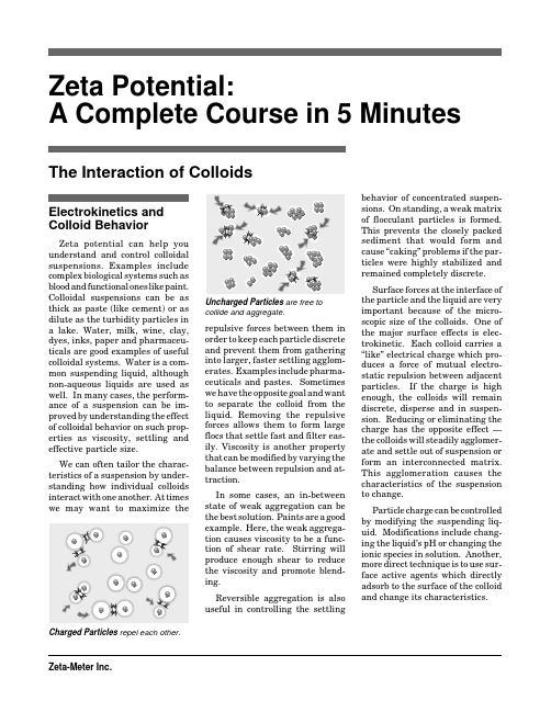
Electrokinetics and Colloid BehaviorZeta potential can help you understand and control colloidal suspensions. Examples include complex biological systems such as blood and functional ones like paint.Colloidal suspensions can be as thick as paste (like cement) or as dilute as the turbidity particles in a lake. Water, milk, wine, clay,dyes, inks, paper and pharmaceu-ticals are good examples of useful colloidal systems. Water is a com-mon suspending liquid, although non-aqueous liquids are used as well. In many cases, the perform-ance of a suspension can be im-proved by understanding the effect of colloidal behavior on such prop-erties as viscosity, settling and effective particle size.We can often tailor the charac-teristics of a suspension by under-standing how individual colloids interact with one another. At times we may want to maximize thebehavior of concentrated suspen-sions. On standing, a weak matrix of flocculant particles is formed.This prevents the closely packed sediment that would form and cause “caking” problems if the par-ticles were highly stabilized and remained completely discrete.Surface forces at the interface of the particle and the liquid are very important because of the micro-scopic size of the colloids. One of the major surface effects is elec-trokinetic. Each colloid carries a “like” electrical charge which pro-duces a force of mutual electro-static repulsion between adjacent particles. If the charge is high enough, the colloids will remain discrete, disperse and in suspen-sion. Reducing or eliminating the charge has the opposite effect —the colloids will steadily agglomer-ate and settle out of suspension or form an interconnected matrix.This agglomeration causes the characteristics of the suspension to change.Particle charge can be controlled by modifying the suspending liq-uid. Modifications include chang-ing the liquid’s pH or changing the ionic species in solution. Another,more direct technique is to use sur-face active agents which directly adsorb to the surface of the colloid and change its characteristics.Uncharged Particles are free to collide and aggregate.repulsive forces between them in order to keep each particle discrete and prevent them from gathering into larger, faster settling agglom-erates. Examples include pharma-ceuticals and pastes. Sometimes we have the opposite goal and want to separate the colloid from the liquid. Removing the repulsive forces allows them to form large flocs that settle fast and filter eas-ily. Viscosity is another property that can be modified by varying the balance between repulsion and at-traction.In some cases, an in-between state of weak aggregation can be the best solution. Paints are a good example. Here, the weak aggrega-tion causes viscosity to be a func-tion of shear rate. Stirring will produce enough shear to reduce the viscosity and promote blend-ing.Reversible aggregation is also useful in controlling the settlingThe Interaction of ColloidsZeta Potential:A Complete Course in 5 MinutesCharged Particlesrepel each other.The diffuse layer can be visualized as a charged atmosphere surrounding the colloid.The Double LayerThe double layer model is used to visualize the ionic environment in the vicinity of a charged colloid and explains how electrical repul-sive forces occur. It is easier to understand this model as a se-quence of steps that would take place around a single negative col-loid if its neutralizing ions were suddenly stripped away.We first look at the effect of the colloid on the positive ions (often called counter-ions) in solution. Initially, attraction from the nega-tive colloid causes some of the posi-tive ions to form a firmly attached layer around the surface of the colloid; this layer of counter-ions isknown as the Stern layer.Additional positive ions are stillattracted by the negative colloid,but now they are repelled by theStern layer as well as by otherpositive ions that are also trying toapproach the colloid. This dynamicequilibrium results in the forma-tion of a diffuse layer of counter-ions. They have a high concentra-tion near the surface which gradu-ally decreases with distance, untilit reaches equilibrium with thecounter-ion concentration in thesolution.In a similar, but opposite, fash-ion there is a lack of negative ionsin the neighborhood of the surface,because they are repelled by thenegative colloid. Negative ions arecalled co-ions because they havethe same charge as the colloid.Their concentration will graduallyincrease with distance, as the re-pulsive forces of the colloid arescreened out by the positive ions,until equilibrium is again reached.The diffuse layer can be visual-ized as a charged atmosphere sur-rounding the colloid. The chargedensity at any distance from thesurface is equal to the difference inconcentration of positive and nega-tive ions at that point. Chargedensity is greatest near the colloidand gradually diminishes towardzero as the concentration of posi-tive and negative ions merge to-gether.The attached counter-ions in theStern layer and the charged at-mosphere in the diffuse layer arewhat we refer to as the doublelayer. The thickness of this layerdepends upon the type and concen-tration of ions in solution.Two Ways to Visualize the Double LayerThe left view shows the change in charge density around the colloid. The right shows the distribution of positive and negative ions around the charged colloid.Zeta PotentialThe double layer is formed in order to neutralize the charged col-loid and, in turn, causes an elec-trokinetic potential between the surface of the colloid and any point in the mass of the suspending liq-uid. This voltage difference is on the order of millivolts and is re-ferred to as the surface potential.The magnitude of the surface potential is related to the surface charge and the thickness of the double layer. As we leave the sur-face, the potential drops off roughly linearly in the Stern layer and then exponentially through the diffuse layer, approaching zero at the imaginary boundary of the double layer. The potential curve is useful because it indicates the strength of the electrical force between par-ticles and the distance at which this force comes into play.A charged particle will move with a fixed velocity in a voltage field.This phenomenon is called electro-phoresis. The particle’s mobility is related to the dielectric constant and viscosity of the suspending liq-uid and to the electrical potential at the boundary between the mov-ing particle and the liquid. This boundary is called the slip plane and is usually defined as the point where the Stern layer and the dif-fuse layer meet. The Stern layer isThe electrokinetic potential between the surface of the colloid and any point in the mass of the suspending liquid is referred to as the surface potential.Zeta Potential vs. Surface Potential The relationship between zeta potential and surface potential depends on the level of ions in the solution.Variation of Ion Density in the Diffuse LayerThe figures above are two representa-tions of the change in charge density through the diffuse layer. One shows the variation in positive and negative ion concentration with distance from a negative colloid. The second shows the net effect — the difference in positive and negative charge density.considered to be rigidly attached to the colloid, while the diffuse layer is not. As a result, the electrical potential at this junction is related to the mobility of the particle and is called the zeta potential .Although zeta potential is an intermediate value, it is sometimes considered to be more significant than surface potential as far as electrostatic repusion is concerned.Zeta potential can be quantified by tracking the colloidal particles through a microscope as they mi-grate in a voltage field.The Balance ofRepulsion & AttractionThe DLVO Theory (named after Derjaguin, Landau, Verwey and Overbeek) is the classical explana-tion of the stability of colloids in suspension. It looks at the balance between two opposing forces — elec-trostatic repulsion and van der Waals attraction — to explain why some colloidal systems agglomer-ate while others do not.Electrostatic repulsion becomes significant when two colloids ap-proach each other and their double layers begin to interfere. Energy is required to overcome this repul-sion. An electrostatic repulsion curve is used to indicate the energy that must be overcome if the par-ticles are to be forced together. It has a maximum value when they are almost touching and decreases to zero outside the double layer.The maximum energy is related to the surface potential and the zeta potential.The DLVO theory explains the tendency of colloids to agglomerate or remain discrete.The height of the barrier indicates how stable the system is. In order to agglomerate, two particles on a collision course must have suffi-cient kinetic energy due to their velocity and mass, to “jump over”this barrier. If the barrier is cleared, then the net interaction is all attractive, and as a result the particles agglomerate. This inner region is after referred to as an energy trap since the colloids can be considered to be trapped together by van der Waals forces.In many cases we can alter the environment to either increase or decrease the energy barrier, de-pending upon our goals. Various methods can be used to achieveElecrostatic Repulsion is always shown as a positive curve.Van der Waals attraction is ac-tually the result of forces between individual molecules in each col-loid. The effect is additive; that is,one molecule of the first colloid has a van der Waals attraction to each molecule in the second colloid. This is repeated for each molecule in the first colloid, and the total force is the sum of all of these. An attrac-tive energy curve is used to indi-cate the variation in van der Waals force with distance between the particles.The DLVO theory explains the tendency of colloids to agglomerate or remain discrete by combining the van der Waals attraction curve with the electrostatic repulsion curve to form the net interaction energy curve. At each distance,the smaller value is subtracted from the larger to get the net energy.The net value is then plotted —above if repulsive and below if at-tractive — and a curve is formed. If there is a repulsive section, then the point of maximum repulsive energy is called the energy barrier.Van der Waals Attraction is shown asa negative curve.subtracting the attraction curve from the repulsion curve.In many cases we can alter the environment to either increase or decrease the energy barrier, depending upon our goals.Effect of Type and Concentration ofElectrolytesSimple inorganic electrolytes can havea significant impact on zeta potential.The effect depends on the relativevalence of the ions and on theirconcentration. Relative valence canalso be thought of as the type ofelectrolyte, with type being the ratiobetween the valences of the cationand the anion.In this example, the zeta potential of adilute suspension of colloidal silica wasmodified by adding different electro-lytes. Aluminum chloride is a 3:1electrolyte and its trivalent cationseasily push the zeta potential towardzero. Contrast this with the effect ofpotassium sulfate, a 1:2 electrolyte.First the zeta potential becomesincreasingly negative until a plateau isreached at about 50 mg/L. At about500 mg/L, the zeta potential begins todecrease because the ions arecompressing the double layer. environment, or pH, or addingsurface active materials to directlyaffect the charge of the colloid. Ineach case, zeta potential measure-ments can indicate the impact ofthe alteration on overall stability.Nothing is ever as simple as itfirst seems. There are other effectsthat must be considered wheneveryou work with particle stability.Steric stabilization is the most sig-nificant one. Usually this involvesthe adsorption of polymers on par-ticle surfaces. You can visualizethe adsorbed layer as a barrieraround each particle, preventingthem from coming close enough forvan der Waals attraction to causeflocculation. Unlike electrostaticstabilization, there are no longrange repulsive forces and the par-ticles are subject to attractive forcesuntil the outer portions of the stericmolecules contact each other.Mechanical bridging by poly-mers can be an effective floccu-lating technique. Some long chainpolymers are large enough to ad-sorb to the surface of several par-ticles at the same time, bindingthem together in spite of the elec-trostatic forces that would normallymake them repel each other.In practice, a combination of ef-fects can be used to create stablesystems or to flocculate them. Forinstance, stable dispersions can becreated by a combination of electro-static repulsion and steric hin-drance. Electronegative disper-sions can be flocculated using longchain cationic polymers which si-multaneously neutralize chargeand bridge between adjacent par-ticles.CeramicsSlip casting is used in volume production of ceramic ware. A sus-pension of clay is prepared and poured into porous molds, which draw off the water from the clay particles by capillary action. A fil-ter cake of clay forms as the water is drawn off. The structure of theControl of Slip CastingClay suspensions for slip casting must have their viscosity minimized so that they pour readily and release trapped air bubbles easily. The above figure shows the effect of pH on the apparent viscosity and zeta potential of thoria (ThO 3). Note that a maximum zeta potential corresponds to a low appar-ent viscosity.Clays & Drilling FluidsClays are an essential part of paper, adhesives, ointments, rub-ber and synthetic plastics. In each of these systems, we have to deal with dispersions of clay in water or other fluids. Clay colloid chemis-try helps us to tailor their charac-teristics to fit the task.Clays are also used as drilling fluids in water well and petroleum well production. They are called drilling muds and are chemically conditioned to vary their proper-ties during drilling. A highly charged suspension is desirable for the initial drilling operation. This keeps the clay colloids discrete, al-lowing them to penetrate into the porous wall of the drilled hole and clog the soil pores, forming a thin,impermeable cake which prevents the loss of drilling fluid. Later, the clay charge may be reduced to form a flocculated suspension in order to keep it from clogging the lower,pumping zone of the well.Minerals & OresMany raw mineral ores such as those for copper, lead, zinc and tungsten are separated by first grinding the ore, mixing it with a collector and suspending it in wa-ter. The next step is flotation. Air is bubbled through the mixture and the collector causes the mineral particles to adhere to the bubbles so that they can be recovered at the surface. The efficiency of this proc-ess depends upon the degree of adsorption between the collector and the mineral and can be con-trolled by the zeta potential of the particles. In another interesting application, zeta potential studies have been used to minimize the viscosity of coal slurries.Determining Point of Zero Charge These experiments with alpha-alumina show good correlation between the point of zero charge as determined by zeta potential and the point of maxi-mum subsidence rate. Subsidence rate is a measure of the degree of coagulation.Zeta Potential ApplicationsAdhesivesAgricultural Chemicals AsbestosAtomic EnergyBeverages Biochemistry BiomedicinePharmaceuticalsThe physical properties of a pharmaceutical suspension affect the user’s response to the product.A successful suspension will not cake and will, therefore enjoy a long shelf life. With fine colloids this can be achieved by adding a suspending agent to increase the zeta potential, and produce maxi-mum repulsion between adjacent particles. This highly dispersed system will settle very slowly, but any that do settle will pack tightly and aggravate caking.Another, and sometimes more effective, approach is to formulate a weakly flocculated suspension. The suspended particles form light, fluffy agglomerates held together by van der Waals forces. The floc-culated particles settle rapidly forming a loosely adhering mass with a large sediment height in-stead of a cake. Gentle agitation will easily resuspend the particles. Weak flocculation requires a zeta potential of almost zero.Fluidization of an AntacidSuspensionFluidization is an alternative toflocculation. A negatively chargedcolloidal polyelectrolyte is used as a“fluidizing” agent. The polyelectrolyteadsorbs onto the surfaces of insolubleparticles and deflocculates them oncethe zeta potential exceeds the criticalvalue.This graph illustrates the fluidization ofan aluminum hydroxide suspensionusing carrageenan sodium as the“fluidizing” agent. The drops in zetapotential and viscosity of the suspen-sion correlate quite well with eachother and are produced by an increasein the concentration of carrageenan.PaintsThe pigments in paint must bewell dispersed in order for the paintto perform successfully. If the pig-ment agglomerates, then the paintwill seem to have larger pigmentparticles and may fail color qual-ity. Gloss and texture are also af-fected by the degree of dispersionbetween the particles in the paint.Zeta potential measurements canbe used in this application to con-trol the composition of the paintand the dosage of additive requiredfor an optimum dispersion.CoalDairy Products DetergentsDry Powder Technology Dyestuffs Emulsions FibersFoodsLatex Production Petrochemicals Petroleum Photographic Emulsions PigmentsWater and Wastewater CoagulationZeta potential is a convenient way to optimize coagulant dosage in water and wastewater treat-ment. The most difficult suspended solids to remove are the colloids. Due to their small size, they easily escape both sedimentation and fil-tration. The key to effective colloid removal is reduction of their zeta potential with coagulants, such as alum, ferric chloride and/or cati-onic polymers. Once the charge is reduced or eliminated, then no re-pulsive forces exist and gentle agi-tation in a flocculation basin causes numerous successful colloid colli-sions. Microflocs form and grow into visible floc particles that settle rapidly and filter easily.PapermakingRetention of fines and fibers canbe increased through zeta poten-tial control. This reduces theamount of sludge produced by thewastewater treatment facility aswell as the load on white waterrecycle systems. Zeta potentialmeasurements also assist the pa-permaker in understanding theeffect of various paper ingredientsas well as the physical characteris-tics of the paper particles them-selves.Zeta Potential Control of Alum DoseThere is no single zeta potential thatwill guarantee good coagulation forevery treatment plant. It will usually bebetween 0 and -10 mV but the targetvalue is best set by test, using pilotplant or actual operating experience.Once the target ZP is established, thenthese correlations are no longernecessary, except for infrequentchecks. Just take a sample from therapid mix basin and measure the zetapotential. If the measured value ismore negative than the target ZP, thenincrease the coagulant dose (and vice-versa).In this example a zeta potential of -3mV corresponds to the lowest filteredwater turbidity and would be used asthe target ZP.Synthetic Size Retention in Paper-makingThe point of maximum size retentioncorresponds to a zeta potential of +4,which can be considered the optimumZP. More positive or more negativevalues of the zeta potential cause adrop in the percent of size retained.Operating at the optimum value resultsin titanium oxide savings, improvedsheet formation, increased wire life,improved sizing, pitch control, andbiocide reduction.Order a CatalogOur catalog describes our instru-ments and accessories in depth, and will help you select the appropriate configuration.Zeta-Meter, Inc.765 Middlebrook AvenuePO Box 3008Staunton, VA 24402, USA Telephone...............540-886-3503 Toll-Free (USA).......800-333-0229 Fax..........................540-886-3728。
Pennsylvania, USA. Part 2 Geochemical controls on constituent concentrations

Dissolved metals and associated constituents in abandonedcoal-mine discharges,Pennsylvania,USA.Part 2:Geochemical controls on constituent concentrationsCharles A.Cravotta IIIU.S.Geological Survey,215Limekiln Road,New Cumberland,PA 17070,United StatesAvailable online 7October 2007AbstractWater-quality data for discharges from 140abandoned mines in the Anthracite and Bituminous Coalfields of Pennsyl-vania reveal complex relations among the pH and dissolved solute concentrations that can be explained with geochemical equilibrium models.Observed values of pH ranged from 2.7to 7.3in the coal-mine discharges (CMD).Generally,flow rates were smaller and solute concentrations were greater for low-pH CMD samples;pH typically increased with flow rate.Although the frequency distribution of pH was similar for the anthracite and bituminous discharges,the bituminous dis-charges had smaller median flow rates;greater concentrations of SO 4,Fe,Al,As,Cd,Cu,Ni and Sr;comparable concen-trations of Mn,Cd,Zn and Se;and smaller concentrations of Ba and Pb than anthracite discharges with the same pH values.The observed relations between the pH and constituent concentrations can be attributed to (1)dilution of acidic water by near-neutral or alkaline ground water;(2)solubility control of Al,Fe,Mn,Ba and Sr by hydroxide,sulfate,and/or carbonate minerals;and (3)aqueous SO 4-complexation and surface-complexation (adsorption)reactions.The forma-tion of AlSO þ4and AlHSO 2þ4complexes adds to the total dissolved Al concentration at equilibrium with Al(OH)3and/or Al hydroxysulfate phases and can account for 10–20times greater concentrations of dissolved Al in SO 4-laden bitumi-nous discharges compared to anthracite discharges at pH of 5.Sulfate complexation can also account for 10–30times greater concentrations of dissolved Fe III concentrations at equilibrium with Fe(OH)3and/or schwertmannite (Fe 8O 8(OH)4.5(SO 4)1.75)at pH of 3–5.In contrast,lower Ba concentrations in bituminous discharges indicate that elevated SO 4concentrations in these CMD sources could limit Ba concentrations by the precipitation of barite (BaSO 4).Coprecip-itation of Sr with barite could limit concentrations of this element.However,concentrations of dissolved Pb,Cu,Cd,Zn,and most other trace cations in CMD samples were orders of magnitude less than equilibrium with sulfate,carbonate,and/or hydroxide minerals.Surface complexation (adsorption)by hydrous ferric oxides (HFO)could account for the decreased concentrations of these divalent cations with increased pH.In contrast,increased concentrations of As and,to a lesser extent,Se with increased pH could result from the adsorption of these oxyanions by HFO at low pH and desorption at near-neutral pH.Hence,the solute concentrations in CMD and the purity of associated ‘‘ochres ”formed in CMD settings are expected to vary with pH and aqueous SO 4concentration,with potential for elevated SO 4,As and Se in ochres formed at low pH and elevated Cu,Cd,Pb and Zn in ochres formed at near-neutral pH.Elevated SO 4content of ochres could enhance the adsorption of cations at low pH,but decrease the adsorption of anions such as As.Such information on envi-ronmental processes that control element concentrations in aqueous samples and associated precipitates could be useful in0883-2927/$-see front matter Published by Elsevier Ltd.doi:10.1016/j.apgeochem.2007.10.003E-mail address:cravotta@Available online at Applied Geochemistry 23(2008)203–226Applied Geochemistrythe design of systems to reduce dissolved contaminant concentrations and/or to recover potentially valuable constituents in mine effluents.Published by Elsevier Ltd.1.IntroductionAbandoned coal-mine discharges(CMD)can becorrosive or encrusting and can impair aquatic hab-itat,water-delivery systems,bridges,and associatedinfrastructure(Barnes and Clarke,1969;Winlandet al.,1991;Earle and Callaghan,1998;Bighamand Nordstrom,2000;Houben,2003).Although dis-solved SO4,Fe,Al,and Mn are widely recognized asmineral constituents of concern,numerous tracemetals have also been documented in CMD,partic-ularly in strongly acidic,low-pH solutions(Hymanand Watzlaf,1997;Rose and Cravotta,1998;Nord-strom and Alpers,1999;Nordstrom,2000;Nord-strom et al.,2000;Cravotta,2008).The dissolvedmetals and associated constituents in CMD can betoxic to aquatic and terrestrial organisms.Generally,the toxicity of a dissolved element increases with itsconcentration after nutritional requirements,ifany,are met(Smith and Huyck,1999).The pH of a solution is an important measure forevaluating aquatic toxicity and corrosiveness.Theseverity of toxicity or corrosion tends to be greaterunder low-pH or high-pH conditions than at near-neutral pH,because the solubility of many metalscan be described as amphoteric,with a greater ten-dency to dissolve as cations at low pH or anionicspecies at high pH(Langmuir,1997).For example,Al hydroxide and aluminosilicate minerals havetheir minimum solubility at pH6–7(Nordstromand Ball,1986;Bigham and Nordstrom,2000),and brief exposure to relatively low concentrationsof dissolved Al can be toxic tofish and other aquaticorganisms(Baker and Schofield,1982;Elder,1988).Accordingly,the U.S.Environmental ProtectionAgency(2000,2002a,b)recommends pH 6.5–9.0for protection of freshwater aquatic life and pH6.5–8.5for public drinking supplies.Nevertheless,pH is not the sole determinant of metals solubility.Anions including SO2À4;HCOÀ3and,less com-monly,ClÀcan be elevated above background con-centrations in CMD(Cravotta,2008),and polyvalent cations such as Al3+and Fe3+tend to associate with such ions of opposite charge(Ball and Nordstrom,1991;Nordstrom,2004).Ion-pair formation,or aqueous-complexation reactions,between dissolved cations and anions can increase the total concentration of metals in a solution at equi-librium with a mineral and can affect the bioavailabil-ity and toxicity of metal ions in aquatic ecosystems (e.g.Rose et al.,1979;Langmuir,1997;Sparks, 2005).Eventually,the solutions can become satu-rated,or reach equilibrium,with respect to various sulfate,carbonate,or hydroxide minerals that estab-lish limits for the dissolved metal concentrations.Dissolved trace elements,such as Pb and Cu,in natural waters can be limited to concentrations lower than expected on the basis of trace-mineral solubility because of surface complexation,or adsorption,of the elements onto solid surfaces (Rose et al.,1979).Hydrous Fe III,Al,and Mn III–IV oxides that precipitate in oxidizing CMD environ-ments are important sorbents because of their large surface areas,tendencies to form colloids and to coat other geological materials,and potential for the oxide surfaces to have variable electrostatic charges(Hem,1977,1978,1985;Loganathan and Burau,1973;McKenzie,1980;Davis and Kent, 1990;Kooner,1993;Coston et al.,1995;Langmuir, 1997;Webster et al.,1998;Kairies et al.,2005; Sparks,2005).Surface hydroxyl groups at the solu-tion interface tend to dissociate at high pH or to protonate at low pH,giving rise to a negative or positive surface charge,respectively.Cations,such as Cd,Cu,Pb,Ni and Zn,tend to be adsorbed by the negatively charged oxide surfaces at near-neu-tral pH,whereas oxyanions,such as sulfate,arse-nate,arsenite,selenate,selenite and borate,tend to be adsorbed by the positively charged surfaces at lower pH(Dzombak and Morel,1990;Davis and Kent,1990;Stumm and Morgan,1996;Drever, 1997;Langmuir,1997).These conditions for adsorption are consistent with reported enrichment of CMD ochres and streambed coatings with Cd, Cu,Pb,Ni and Zn at near-neutral pH and with S and As at low pH(Winland et al.,1991;Hedin et al.,1994;Rose and Ghazi,1997;Cravotta and Trahan,1999;Cravotta and Bilger,2001;Cravotta et al.,2001;Hedin,2003;Kairies et al.,2005;Crav-otta,2005,2008).This report examines relationships between pH, SO4,and metal concentrations in CMD samples204 C.A.Cravotta III/Applied Geochemistry23(2008)203–226from abandoned coal mines in the Bituminous and Anthracite Coalfields of Pennsylvania.Similarities and differences in theflow rate and chemistry between the anthracite and bituminous CMD sam-ples are examined.The potential formation of aque-ous complexes,surface complexes,and stability of possible solid phases in contact with aqueous solu-tions are evaluated with respect to thermodynamic equilibrium at near-surface temperature and pres-sure conditions.Additionally,ratios of Br/Cl are used to evaluate potential for mixing of fresh ground water with road salts or deep brine.A companion report by Cravotta(2008)describes the chemical and hydrological data in more detail and examines the correlations betweenflow rate,pH,constituent concentrations,and constituent loadings.2.Methods of sampling and analysisThe study area description,a map showing the sampling locations,and details on the site character-istics and methods of data collection and chemical analysis are given in the companion report by Crav-otta(2008).Essential information on sampling and analytical methods is summarized below.2.1.Water-quality sampling and analysisIn summer and fall1999,water-quality samples from140abandoned,discharging coal mines in the Anthracite and Bituminous Coalfields of Penn-sylvania were collected by the U.S.Geological Sur-vey(USGS)for analysis of chemical concentrations and loading.The140discharges,including99from bituminous mines and41from anthracite mines, were selected among thousands of CMD sources statewide based on their geographic distribution, accessibility,and potential for substantial loadings of dissolved metals.Most of the sampled discharges were from underground mines.All the CMD sources were discharging by gravity when sampled. Flow was measured at each site by use of a current meter or bucket and stopwatch.To minimize effects from aeration,electrodes were immersed and samples were collected as close as possible to the point of discharge.Field data forflow rate,temperature,specific conductance (SC),dissolved O2(DO),pH and redox potential (Eh)were measured at each site when samples were collected in accordance with standard methods (Rantz et al.,1982a,b;Wood,1976;U.S.Geological Survey,variously dated;Ficklin and Mosier,1999).All meters were calibrated in thefield using elec-trodes and standards that had been thermally equil-ibrated to sample temperatures.Field pH and Eh were determined using a combination Pt and Ag/ AgCl electrode with a pH sensor.The electrode was calibrated in pH2.0,4.0and7.0buffer solu-tions and in ZoBell’s solution(Wood,1976;U.S. Geological Survey,variously dated).Values for Eh were corrected to25°C relative to the standard hydrogen electrode in accordance with methods of Wood(1976)and Nordstrom(1977).An unfiltered subsample for analysis of alkalinity was capped leaving no head space and stored on ice.Alkalinity was analyzed in the laboratory within 48h of sampling by titration with H2SO4to the end-point pH of4.5(American Public Health Associa-tion,1998;Kirby and Cravotta,2005a,b).The pH before and during alkalinity titrations was measured using a liquid-filled combination Ag/AgCl pH elec-trode calibrated in pH4.0,7.0,and10.0buffer solu-tions.The net acidity of the CMD samples was computed fromfield pH,alkalinity and dissolved Fe,Mn,and Al concentrations(Kirby and Cravotta, 2005b;Cravotta,2008).Subsamples for analysis of‘‘dissolved”constitu-ents werefiltered through a0.45-l m pore-size nitro-cellulose capsulefilter using the clean-sampling methods of Horowitz et al.(1994).Although colloi-dal particles could pass through0.45-l m pore-sizefil-ters,constituent concentrations in thefiltered samples are interpreted hereinafter as dissolved sol-utes.The subsample for cation analyses was pre-served with trace-element grade HNO3to pH<2. Anions(SO4,Cl,F,NO3,NO2and PO4)infiltered, refrigerated samples were analyzed by ion chroma-tography(IC)(Fishman and Friedman,1989;Crock et al.,1999).Concentrations of major cations and trace metals in thefiltered,acidified samples were determined using inductively coupled plasma optical emission spectroscopy(ICP-OES)and inductively coupled plasma mass spectrometry(ICP-MS)(Fish-man and Friedman,1989;Crock et al.,1999).Results for replicate analyses were averaged before evalua-tion.When values for one or more replicates were reported as not detected,the lowest reported value or the lowest non-detect value was used as the result.putation of aqueous complexation and mineral saturationActivities of aqueous species,partial pressure of CO2(P CO2),and mineral-saturation index(SI)C.A.Cravotta III/Applied Geochemistry23(2008)203–226205values were calculated using the WATEQ4F version 2.63computer program(Ball and Nordstrom, 1991).The activities of Fe II and Fe III species were computed on the basis of the measured Eh,Fe con-centration,and temperature of the samples.Nord-strom(1977)and Nordstrom et al.(1979)have shown there is good agreement between the mea-sured Eh and that predicted by the Fe II/Fe III couple in acidic mine waters.For the90samples that hadalkalinity>0,the P CO2was computed on the basisof measured pH,alkalinity,and -puted SI values for silicate,oxide,carbonate and sulfate minerals that could be present in coal depos-its or associated wall rocks or that may form as solutions oxidized or evaporated at the land surface were summarized as a function of pH.Stability diagrams were developed to evaluate the potential for equilibrium of specific elements(Ca, Mg,Al,Fe,Mn,Ba,Cd,Cu,Pb,Sr,Zn)with respect to hydroxide,sulfate and carbonate minerals(solubility)for specified ranges of pH,Eh,P CO2,SO4and Cl.The theoretical stability boundaries for min-erals and aqueous species computed with spread-sheet models were plotted as reference lines or curves on‘‘pC–pH”and‘‘Eh–pH”diagrams(e.g. Snoeyink and Jenkins,1981;Drever,1997;Lang-muir,1997).Then,data on sample pH,Eh,or activ-ities of uncomplexed cations(Al3+,Fe3+,Fe2+)and major aqueous complexes computed with WATEQ4F were plotted as points on the stability diagrams.Reactions and associated equilibrium constants for relevant species and solids in the spreadsheet models were obtained mostly from the WATEQ4F thermodynamic database(Nordstrom et al.,1990;Ball and Nordstrom,1991;Drever, 1997)and supplemented with other data for Fe III minerals(Bigham et al.,1996;Yu et al.,1999).Ther-modynamic data that were used are summarized in the Appendix(Tables A1–A3).Equilibrium reac-tions and associated thermodynamic data for hydroxide,sulfate,and carbonate minerals and aqueous species involving SO4,CO3,Fe III and Al are given in Table A1.Speciation and solubility data for Al,Ba,Ca,Cd,Co,Cu,Fe II,Fe III,Mg,Mn II, Ni,Pb II,Sr and Zn are summarized in Table A2; detailed reactions for Pb II with data from Table A2are provided as an example in Table A3.putation of surface complexationAdsorption and desorption,or surface complexa-tion,of cations and anions on hydrous ferric hydroxide(HFO)particles were evaluated using adiffuse double-layer modeling approach with PHREEQC(Parkhurst and Appelo,1999),sur-face-complexation data from Dzombak and Morel (1990),and aqueous speciation data from Ball and Nordstrom(1991).Although the concentrations of dissolved solutes in the models could be specified based on the known ranges for the CMD samples, knowledge of the amounts and properties of the sor-bent HFO was lacking.Models were developed for different cations and anions byfirst modifying an example for Zn adsorption on HFO(‘‘example8”of Parkhurst and Appelo,1999)that implicitly spec-ified the HFO surface assemblage in equilibrium with a solution offixed composition.The HFO solid was specified as0.09g kgÀ1solution,with a specific surface area of600m2gÀ1consisting of5Â10À6 moles of strong binding sites and2Â10À4moles of weak binding sites.With data from Dzombak and Morel(1990),additional sorbate elements were considered(cations:Ba,Ca,Cd,Co,Cu,Mn II,Ni, Pb II,Sr;anions:As,B,Cr,Se,S,V).Aqueous spe-ciation and adsorption distribution were computed for a constant concentration of the sorbate element and a range of pH values.Plots were created to summarize the percentage of the sorbate element distributed between the solution and sorbent as a function of pH.The models developed for anion adsorption simulated a NaCl background matrix, whereas those for cation adsorption also specified initial concentrations of SO2À4and HCOÀ3to iden-tify effects of metal complexes with OHÀ,ClÀ,SO2À4and CO2À3species.3.Results–characteristics of anthracite and bituminous CMD samplesData on theflow rates,pH,acidity,alkalinity and selected solute concentrations for the140 CMD samples collected in1999from abandoned coal mines in the Anthracite and Bituminous Coal-fields of Pennsylvania are summarized in Table1 and Figs.1and2.Sampledflow rates at the140 CMD sites ranged from0.028to2.210L sÀ1.The anthracite discharges had greater medianflow rates than the bituminous discharges(Table1).Further-more,median and maximumflow rates for the anthracite mine discharges generally exceeded those for the bituminous mines for the same pH class interval(Fig.1).Generally,flow rate and alkalinity increased with pH,whereas acidity,SO4and metal concentrations206 C.A.Cravotta III/Applied Geochemistry23(2008)203–226decreased(Fig.1).These trends imply(1)neutral-ization of CMD did not result solely by mineral dis-solution but also involved dilution of initially acidic water by alkaline ground water or surface water or (2)decreased pyrite oxidation because of decreased contact time with increasedflows.Regardless of the cause,mines with largeflows tended to be less acidic and have greater pH than those with smallflows. Largerflow rates for anthracite discharges than bituminous discharges reflect differences in the phys-iographic and geologic settings between the two coalfields(Berg et al.,1989;Edmunds,1999;Eggle-ston et al.,1999)and indicate that,on average,the anthracite mines have larger recharge areas and more extensiveflooded volumes compared to the bituminous mines.Because anthracite mine com-plexes historically connected multiple coalbeds and extended beneath valleys to hundreds of meters below the regional water table,their mined areas and associated discharge volumes tend to be sub-stantially greater than those from contemporaneous surface mines or bituminous mines that access one or two coalbeds within isolated hilltops.Thefield pH of the140CMD samples ranged from 2.7to7.3,with the majority either acidic (pH 2.5–4)or near neutral(pH6–7)(Table1, Fig.1).This bimodal frequency distribution of pH for the CMD samples was discussed in detail by Cravotta et al.(1999)and Kirby and Cravotta (2005a,b).Although the minimum and maximum pH values were associated with bituminous mine discharges,the median pH values of5.1and5.2 were similar for the41anthracite and99bituminous discharges,respectively(Table1).Table1Summary of hydrochemical characteristics of discharges from140abandoned coal mines in Pennsylvania,1999aCoalfield and number of samples Flowrate(L sÀ1)Temperature(°C)Specific(l S cmÀ1)Redoxpotential,Eh(mV)pH,field Alkalinity(mg LÀ1asCaCO3)Net acidity b(mg LÀ1asCaCO3)Hardness c(mg LÀ1asCaCO3)Sulfate,SO4(mg LÀ1)Anthracite N=4164.011.4692390 5.1343244260 (0.028;2.21)(8.8;26.6)(131;2050)(170;770)(3.0;6.3)(0;120)(À79;588)(23;770)(34;1300)Bituminous N=9912.512.01480390 5.21476433580(0.227;278)(9.0;16.5)(495;3980)(140;800)(2.7;7.3)(0;510)(À326;1587)(117;1811)(120;2000)Calcium,Ca(mg LÀ1)Magnesium,Mg(mg LÀ1)Sodium,Na(mg LÀ1)Potassium,K(mg LÀ1)Chloride,Cl(mg LÀ1)Silica,SiO2(mg LÀ1)Aluminum,Al(mg LÀ1)Iron,Fe(mg LÀ1)Manganese,Mn(mg LÀ1)Anthracite N=413735 6.1 1.8 6.3130.2815 2.9(3.3;180)(3.6;87)(0.69;67)(0.7;3.9)(0.1;110)(5.8;51)(0.007;26)(0.046;312)(0.019;19)Bituminous N=991103823 3.37.719 1.543 2.3 (19;410)(8.5;210)(1.0;500)(0.5;12)(0.4;460)(8.2;67)(0.008;108)(0.16;512)(0.12;74) Arsenic,As(l g LÀ1)Barium,Ba(l g LÀ1)Cadmium,Cd(l g LÀ1)Copper,Cu(l g LÀ1)Lead,Pb(l g LÀ1)Nickel,Ni(l g LÀ1)Selenium,Se(l g LÀ1)Strontium,Sr(l g LÀ1)Zinc,Zn(l g LÀ1)Anthracite N=410.62180.120.850.68830.4190130(<0.03;15)(13;31)(<0.01;2.1)(0.4;91)(<0.05;11)(19;620)(<0.2;3.9)(27;2700)(3.0;1000)Bituminous N=992.0130.12 2.20.10900.61000140 (0.1;64)(2.0;39)(<0.01;16)(0.4;190)(<0.05;4.6)(2.6;3200)(<0.2;7.6)(47;3600)(0.6;10,000)a Median(minimum;maximum);L sÀ1,liters per second;°C,degrees Celsius;l S cmÀ1,microsiemens per centimeter;mV,millivolts; mg LÀ1,milligrams per liter;l g LÀ1,micrograms per liter.Sample site locations shown in Fig.1of Cravotta(2008).Detailed data available from Cravotta(2008).b Net acidity=(acidity,computedÀAlkalinity,measured)per Kirby and Cravotta(2005b).Acidity,computed(mg LÀ1 CaCO3)=50Á(10(3ÀpH)+3ÁC Al/26.98+2ÁC Fe/55.85+2ÁC Mn/54.94),where C Al,C Fe,and C Mn are dissolved aluminum,iron,and manganese concentration,respectively,in milligrams per liter.c Hardness(mg LÀ1CaCO3)=2.5ÁC Ca+4.1ÁC Mg,where C Ca and C Mg are dissolved calcium and magnesium concentration, respectively,in milligrams per liter.C.A.Cravotta III/Applied Geochemistry23(2008)203–226207Alkalinity concentrations ranged from0 (pH64.4;50samples)to510mg LÀ1as CaCO3 (Table1).Computed net acidity concentrations, which exclude contributions from dissolved CO2, ranged fromÀ326to1587mg LÀ1as CaCO3(Table 1).Concentrations of dissolved SO4(34–2000 mg LÀ1),Fe(0.046–512mg LÀ1),Al(0.007–108 mg LÀ1)and Mn(0.019–74mg LÀ1)varied signifi-cantly(Table1).Generally,the highest concentra-tions of acidity,SO4,Fe,Al,Mn and most other metals were associated with low-pH samples. Although a few samples were saturated with DO (10–12mg LÀ1),median concentrations of DO gener-ally were low(<2mg LÀ1)throughout the range of pH(Fig.1),consistent with the predominance of dis-solved Fe II and Mn II species in most CMD samples.The bituminous discharges generally contained greater concentrations of total dissolved solids than the anthracite discharges as a whole(Table1)or with the same pH values(Figs.1and2)as indicated by greater median and maximum values for specific conductance and concentrations of alkalinity,acid-ity,hardness,SO4,Fe,Al,Mn,and other solutes, including Cd,Cu,Ni,Sr and Zn.In contrast,the median concentrations of dissolved Ba and Pb in bituminous discharges were less than those for the anthracite discharges(Table1,Fig.2).As noted above,relatively low concentrations of dissolved mineral constituents in the anthracite discharges could result from dilution of initially acidic CMD with a freshwater source containing limited dis-solved solids.Such dilution could affect aqueous speciation and mineral solubilities.4.Discussion–geochemical controls on constituent concentrationsThe widespread occurrence of SO4,Fe,Mn,Al, As,Ba,Cd,Cu,Pb,Ni,Se,Sr and Zn in CMD sam-ples(Figs.1and2)results from the mobilization of these constituents by the weathering of pyrite and associated minerals in coal and surrounding sedimen-tary wall rocks.Under oxidizing conditions,pyrite oxidation produces H2SO4that reacts with carbon-208 C.A.Cravotta III/Applied Geochemistry23(2008)203–226ate,silicate and oxide minerals along pathways downflow from the pyrite (e.g.Cravotta,1994;Blowes and Ptacek,1994).Generally,the pH,alka-linity,and concentrations of alkali and alkaline earth cations increase because of the wall rock reactions,whereas SO 4concentrations remain constant.On the other hand,reducing conditions also can lead to increased pH but with corresponding decreases in the concentrations of SO 4and certain metals (Stumm and Morgan,1996;Drever,1997;Langmuir,1997).Hence,concentrations of dissolved metals and other trace constituents can increase or decrease as the CMD approaches neutrality.Such variations in sol-ute concentrations can be explained by geochemical processes including oxidation and reduction,mineral dissolution and precipitation,aqueous-complexa-tion,and surface-complexation (adsorption and desorption)reactions.4.1.Aqueous complexation and mineral solubility controls of constituents in CMD samplesAlthough Fe III and Al hydroxide minerals are insoluble at near-neutral pH,most divalent cations,including Fe II ,Mn,Cu,Cd,Pb and Zn,form rela-tively soluble hydroxides (Fig.3).Precipitation of Cu II ,Fe II ,and other divalent metal hydroxides gen-erally will not limit the dissolved metal concentra-tions until solutions become highly alkaline (pH >9).Furthermore,as demonstrated later,aqueouscomplexation with SO 2À4;CO 2À3;HCO À3;Cl À,and/or other anions can increase the dissolved metal concentration at equilibrium with its hydroxide.Nevertheless,observed concentrations of dissolved Fe II ,Cu,Cd,Pb,Zn,and other trace metals tend to be substantially lower than these solubility limits.Within the pH range of CMD,many trace metals can be adsorbed by hydrous Fe III ,Al and Mn IV oxi-des (e.g.Dzombak and Morel,1990;Davis and Kent,1990;Kooner,1993;Coston et al.,1995;Web-ster et al.,1998)and/or precipitate as sulfate or car-bonate minerals.Although most trace metals are capable of forming pure sulfate or carbonate phases,Cd,Cu,Pb,Zn,Ba and Sr commonly sub-stitute for Ca,Mg and Fe in calcite (CaCO 3),arago-nite (CaCO 3),dolomite (CaMg(CO 3)2),ankerite (Ca(Fe,Mg)(CO 3)2)and siderite (FeCO 3)(Hanshaw and Back,1979;Veizer,1983;Mozley,1989).2 945 23 15 1313114 713 91818217.52.53.0 3.54.0 4.55.0 5.56.0 6.57.025034568101520253040B A R I U M ,μg .L -1294523 15 1 3 1311471391818 2 1200.050.070.10.20.30.50.712357107.52.53.0 3.54.0 4.55.0 5.56.0 6.57.0L E A D ,μg .L -12 9 4 5 2 315 1 313 11 4 713 91818 210.220,0000.51251020501002005001,0002,0005,00010,000Z I N C ,μg .L -17.52.53.0 3.54.0 4.55.0 5.56.0 6.57.029452315131311471391818217.52.53.0 3.54.0 4.55.0 5.56.0 6.57.00.012000.020.050.10.20.5125102050100A R S E N I C ,μg .L -1pH CLASS INTERVAL MIDPOINT pH CLASS INTERVAL MIDPOINT pH CLASS INTERVAL MIDPOINT29452315131311471391818210.3300.0.50.7123571020305070100200C O P P E R , μg .L -17.52.53.0 3.54.0 4.55.0 5.56.0 6.57.0294523151313114713918182155,000710203050701002003005007001,0002,0003,000N I C K E L ,μg .L -17.52.53.0 3.54.0 4.55.0 5.56.0 6.57.029452315131311471391818210.003300.0050.010.020.030.050.10.20.30.512351020C A D M I U M , μg .L -17.52.53.0 3.54.0 4.55.0 5.56.0 6.57.0S E L E N I U M ,μg .L -17.52.5 3.0 3.5 4.0 4.5 5.0 5.5 6.0 6.57.029452315131311471391818210.07100.10.20.30.40.50.71234572945231513131147139181821205,0003050701002003005007001,0002,0003,000S T R O N T I U M ,μg .L -17.52.53.0 3.54.0 4.55.0 5.56.0 6.57.0Fig. 2.Boxplots showing concentrations of selected trace elements as a function of pH for 140abandoned mine discharges in Pennsylvania,1999:(A)As;(B)Ba;(C)Cd;(D)Cu;(E)Pb;(F)Ni;(G)Se;(H)Sr;(I)Zn.Shaded box,bituminous;open box,anthracite.C.A.Cravotta III /Applied Geochemistry 23(2008)203–226209。
藤壶附着对低合金高强度钢牺牲阳极保护效果的影响

表面技术第52卷第8期腐蚀与防护藤壶附着对低合金高强度钢牺牲阳极保护效果的影响蔡凡帆1,2,3,4,黄彦良1,2,4,邢少华5,许勇1,2,3,4,王秀通1,2,4(1.中国科学院海洋研究所 海洋环境腐蚀与生物污损重点实验室,山东 青岛 266071;2.青岛海洋科学与技术国家实验室海洋腐蚀与防护开放工作室,山东 青岛 266237;3.中国科学院大学,北京 100049;4.中国科学院海洋大科学研究中心,山东 青岛 266071;5.中国船舶重工集团公司第七二五研究所,山东 青岛 266237)摘要:目的探索藤壶附着对低合金高强度钢阴极保护效果的影响,研究海洋中大型污损生物附着下金属材料的腐蚀规律。
方法在青岛胶州湾进行腐蚀挂板实海暴露实验,运用纱网箱隔离藤壶幼虫作为对照组。
在暴露6个月和12个月后回收腐蚀挂板,研究藤壶附着后挂板腐蚀形貌、腐蚀产物和阴极保护效率的变化。
在室内进行模拟实验,研究牺牲阳极对存在藤壶附着的钢的保护效果。
结果在施加牺牲阳极保护后,藤壶附着下的钢表面具有更明显的局部腐蚀坑,且多位于藤壶附着的边缘位置。
藤壶附着对牺牲阳极保护效率的影响有限,藤壶附着钢的极化电位相较于无藤壶附着钢的极化电位更负,保护电流密度更小。
藤壶附着钢的未附着区域的保护电流密度(63.9 μA/cm2)比无藤壶附着钢(46.3 μA/cm2)的保护电流密度高。
XRD 谱、拉曼光谱和SEM图表明,藤壶附着不影响腐蚀产物或沉积物的组成。
结论在牺牲阳极保护下,处于藤壶附着边缘和中心位置的钢,可作为氧浓差电池的阳极,在自催化的协同作用下,腐蚀过程加速,形成了严重的局部腐蚀。
同时,藤壶附着可使钢的有效工作面积下降,导致藤壶附着下钢试样的无藤壶附着区域与不存在藤壶附着的钢试样相比,具有更高的保护电流密度和更负的极化电位。
关键词:藤壶;低合金高强度钢;牺牲阳极;局部腐蚀;保护效率;遮蔽作用中图分类号:TG174.41 文献标识码:A 文章编号:1001-3660(2023)08-0226-11DOI:10.16490/ki.issn.1001-3660.2023.08.017Effect of Barnacle Adhesion on Cathodic Protection of Low AlloyHigh Strength Steel by Sacrificial AnodeCAI Fan-fan1,2,3,4, HUANG Yan-liang1,2,4, XING Shao-hua5,XU Yong1,2,3,4, WANG Xiu-tong1,2,4(1. Key Laboratory of Marine Environmental Corrosion and Bio-fouling, Institute of Oceanology, Chinese Academy of Science,Shandong Qingdao 266071, China; 2. Open Studio for Marine Corrosion and Protection, Qingdao National Laboratory for收稿日期:2022-07-29;修订日期:2022-09-19Received:2022-07-29;Revised:2022-09-19基金项目:国家自然科学基金(41976033)Fund:National Natural Science Foundation of China (41976033)作者简介:蔡凡帆(1998—),男,硕士,主要研究方向为生物污损。
the hydrogen bond in the solid state
1.IntroductionThe hydrogen bond was discovered almost 100years ago,[1]but still is a topic of vital scientific research.The reason forthis long-lasting interest lies in the eminent importance ofhydrogen bonds for the structure,function,and dynamics of avast number of chemical systems,which range from inorganicto biological chemistry.The scientific branches involved arevery diverse,and one may include mineralogy,materialscience,general inorganic and organic chemistry,supramo-lecular chemistry,biochemistry,molecular medicine,andpharmacy.The ongoing developments in all these fields keepresearch into hydrogen bonds developing in parallel.In recentyears in particular,hydrogen-bond research has stronglyexpanded in depth as well as in breadth,new concepts havebeen established,and the complexity of the phenomenaconsidered has increased dramatically.This review is intendedto give a coherent survey of the state of the art,with a focus onthe structure in the solid state,and with weight put mainly on the fundamental aspects.Numerous books [2±9]and reviews on the subject have appeared earlier,so a historical outline is not necessary.Much of the published numerical material is somewhat outdated and,therefore,this review contains some numerical data that have been newly retrieved from the most relevant structural database,the Cambridge Structural Data-base (CSD).[10]It is pertinent to recall here the earlier ™classical∫view on hydrogen bonding.One may consider the directional inter-action between water molecules as the prototype of all hydrogen bonds (Scheme 1,definitions of geometric parameters are also in-cluded).The large difference in electro-negativity between the H and O atoms makes the O ÀH bonds of a water molecule inherently polar,with partial atomic charges of around 0.4on each H atom and À0.8on the O atom.Neighboring water molecules orient in such a way that local dipoles O d ÀÀH d point at negative partial charges O d À,that is,at the electron lone pairs of the filled p orbitals.In the resulting The Hydrogen Bond in the Solid StateThomas Steiner*In memory of JanKroon[*]Dr.T.SteinerInstitut f¸r Chemie–KristallographieFreie Universit‰t BerlinTakustrasse 6,14195Berlin (Germany)Fax:( 49)30-838-56702E-mail:steiner@chemie.fu-berlin.deREVIEWSREVIEWS T.SteinerOÀH¥¥¥j O interaction,the intermolecular distance is short-ened by around1äcompared to the sum of the van der Waals radii for the H and O atoms[11](1ä 100pm),which indicates there is substantial overlap of electron orbitals to form a three-center four-electron bond.Despite significant charge transfer in the hydrogen bond,the total interaction is dominantly electrostatic,which leads to pronounced flexibil-ity in the bond length and angle.The dissociation energy is around3±5kcal molÀ1.This brief outline of the hydrogen bond between water molecules can be extended,with only minor modifications,to analogous interactions XÀH¥¥¥A formed by strongly polar groups X dÀÀH d on one side,and atoms A dÀon the other (X O,N,halogen;A O,N,S,halide,etc.).Many aspects of hydrogen bonds in structural chemistry and structural biology can be readily explained at this level,and it is certainly the relative success of these views that made them dominate the perception of the hydrogen bond for decades.This dominance has been so strong in some periods that research on hydrogen bonds differing too much from the one between water molecules was effectively impeded.[8]Today,it is known that the hydrogen bond is a much broader phenomenon than sketched above.What can be called the™classical hydrogen bond∫is just one among many–a very abundant and important one,though.We know of hydrogen bonds that are so strong that they resemble covalent bonds in most of their properties,and we know of others that are so weak that they can hardly be distinguished from van der Waals interactions.In fact,the phenomenon has continuous transition regions to such different effects as the covalent bond,the purely ionic,the cation±p,and the van der Waals interaction.The electrostatic dominance of the hydrogen bond is true only for some of the occurring configurations,whereas for others it is not.The H¥¥¥A distance is not in all hydrogen bonds shorter than the sum of the van der Waals radii.For an XÀH group to be able to form hydrogen bonds,X does not need to be™very electroneg-ative∫,it is only necessary that XÀH is at least slightly polar. This requirement includes groups such as CÀH,PÀH,and some metal hydrides.XÀH groups of reverse polarity, X d ÀH dÀ,can form directional interactions that parallel hydrogen bonds(but one can argue that they should not be called so).Also,the counterpart A does not need to be a particularly electronegative atom or an anion,but only has to supply a sterically accessible concentration of negative charge. The energy range for dissociation of hydrogen bonds covers more than two factors of ten,about0.2to40kcal molÀ1,and the possible functions of a particular type of hydrogen bond depend on its location on this scale.These issues shall all be discussed in the following sections.For space reasons,it will not be possible to cover all aspects of hydrogen bonding equally well.Therefore,some important fields,for which recent guiding reviews are available,will not be discussed in great length.One example is the role of hydrogen bonds in molecular recognition patters(™supra-molecular synthons∫),[12]and the use of suitably robust motifs for the construction of crystalline archtitectures with desired properties(™crystal engineering∫).[13,14]This area includes the interplay of hydrogen bonds with other intermolecular forces, with whole arrays of such forces,and hierarchies within such an interplay.The reader interested in this complexfield is referred to the articles of Desiraju,[12,13]Leiserowitz et al.,[15] and others.[16]A further topic which could not be covered here is the symbolic description of hydrogen bond networks using tools of graph theory,[17]in particular the™graph set analy-sis∫.[18]An excellent guiding review is also available in this case.[19]For hydrogen bonding in biological structures,the interested reader is referred to the book of Jeffrey and Saenger,[5]and for theoretical aspects to the book of Scheiner[7]as well as other recent reviews.[20]Results obtained with experimental methods other than diffraction will be touched upon only briefly,and will possibly leave some readers dissatisfied.The role of hydrogen bonding in special systems will not be discussed at all,simply because there are too many of them.2.Fundamentals2.1.Definition of the Hydrogen BondBefore discussing the hydrogen bond itself,the matter of hydrogen bond definitions must be addressed.This is an important point,because definitions of terms often limit entire fields.It is,also,a problematic point because very different hydrogen bond definitions have been made,and partREVIEWS Solid-State Hydrogen Bondsof the literature relies quite uncritically on the validity(or thevalue)of the particular definition that is adhered to.Time has shown that only very general and flexibledefinitions of the term™hydrogen bond∫can do justice tothe complexity and chemical variability of the observedphenomena,and include the strongest as well as the weakestspecies of the family,and inter-as well as intramolecularinteractions.A far-sighted early definition is that of Pimenteland McClellan,who essentially wrote that™...a hydrogenbond exists if1)there is evidence of a bond,and2)there isevidence that this bond sterically involves a hydrogen atomalready bonded to another atom∫.[2]This definition leaves thechemical nature of the participants,including their polaritiesand net charges,unspecified.No restriction is made on theinteraction geometry except that the hydrogen atom must besomehow™involved∫.The crucial requirement is the existenceof a™bond∫,which is itself not easy to define.The methods totest experimentally if requirements1and2are fulfilled arelimited.For crystalline compounds,it is easy to see withdiffraction experiments whether an H atom is involved,but itis difficult to guarantee that a given contact is actually™bonding∫.A drawback of the Pimentel and McClellan definition isthat in the strict sense it includes pure van der Waals contacts(which can be clearly™bonding∫,with energies of severaltenths of a kcal molÀ1),and it also includes three-center two-electron interactions where electrons of an XÀH bond are donated sideways to an electron-deficient center(™agosticinteraction∫).From a modern viewpoint,it seems advisable tomodify point2,such as by requiring that XÀH acts as a proton (not electron)donor.Therefore,the following definition is proposed:An XÀH¥¥¥A interaction is called a™hydrogen bond∫,if 1.it constitutes a local bond,and2.XÀH acts as proton donor to A.The second requirement is related to the acid/base proper-ties of XÀH and A,and has the chemical implication that a hydrogen bond can at least in principle be understood as an incipient proton-transfer reaction from XÀH to A.It excludes, for example,pure van der Waals contacts,agostic interactions, so-called™inverse hydrogen bonds∫(see Section8),and B-H-B bridges.As a matter of fact,point2should be interpreted liberally enough to include symmetric hydrogen bonds XÀHÀX,where donor and acceptor cannot be distin-guished.The direction of formal or real electron transfer in a hydrogen bond is reverse to the direction of proton donation.Apart from general chemical definitions,there are manyspecialized definitions of hydrogen bonds that are based oncertain sets of properties that can be studied with a particulartechnique.For example,hydrogen bonds have been definedon the basis of interaction geometries in crystal structures(short distances,fairly™linear angles∫q),certain effects in IRabsorption spectra(red-shift and intensification of n XH,etc.),or certain properties of experimental electron density distri-butions(existence of a™bond critical point∫between H andA,with numerical parameters within certain ranges).All suchdefinitions are closely tied to a specific technique,and may be quite useful in the regime accessible to it.Nevertheless,theyare more or less useless outside that regime,and many amisunderstanding in the hydrogen bond literature has beencaused by applying such definitions outside their region ofapplicability.The practical scientist often requires a technical definition,and automated data treatment procedures for identifyinghydrogen bonds cannot be done without.It is not within thescope of this article to discuss any set of threshold values thata™hydrogen bond∫must pass in any particular type oftechnical definition.It is only mentioned that the™van derWaals cutoff∫definition[21]for identifying hydrogen bonds ona structural basis(requiring that the H¥¥¥A distance issubstantially shorter than the sum of the van der Waals radiiof H and A)is far too restrictive and should no longer beapplied.[5,6,8]If distance cutoff limits must be used,XÀH¥¥¥A interactions with H¥¥¥A distances up to3.0or even3.2äshould be considered as potentially hydrogen bonding.[6]Anangular cutoff can be set at>908or,somewhat moreconservatively,at>1108.A necessary geometric criterionfor hydrogen bonding is a positive directionality preference,that is,linear XÀH¥¥¥A angles must be statistically favored over bent ones(this is a consequence of point2of the above definition).[22]2.2.Further TerminologyA large part of the terminology concerning hydrogen bonds is not uniformly used in the literature,and still today, terminological discrepancies lead to misunderstanding be-tween different authors.Therefore,some of the technical terms used in this review need to be explicitly defined.In a hydrogen bond XÀH¥¥¥A,the group XÀH is called the donor and A is called the acceptor(short for™proton donor∫and™proton acceptor∫,respectively).Some authors prefer the reverse nomenclature(XÀH electron acceptor,Y electron donor),which is equally justified.In a simple hydrogen bond,thedonor interacts with one acceptor(Scheme2a).Since the hydro-gen bond has a long range,adonor can interact with two andthree acceptors simultaneously(Scheme2b,c).Hydrogen bondswith more than three acceptorsare possible in principle,but areonly rarely found in practice be-cause they require very highspatial densities of acceptors.The terms™bifurcated∫and™tri-furcated∫are commonly used todescribe the arrangements inScheme2b and c,respectively.The term™two-centered∫hydro-gen bond is an alternative descrip-tor for XÀH¥¥¥A(Scheme2a)where the H-atom is bonded totwo other atoms,and is itself notX H AX HAX H AAAAb)c)a)dd1d2d1d2d3Scheme2.Different typesof hydrogen bridges.a)Nor-mal hydrogen bond with oneacceptor.b)Bifurcated hy-drogen bond;if the twoH¥¥¥A separations are dis-tinctly different,the shorterinteraction is called majorcomponent,and the longerone the minor component ofthe bifurcated bond.c)Tri-furcated hydrogen bond.REVIEWST.Steiner counted as a center.Consequently,the arrangements in Scheme 2b and 2c may be called ™three-∫and ™four-centered∫hydrogen bonds,respectively.[5,6]This terminology is logical,but leads to confusion from the point of view of regarding hydrogen bonds O ÀH ¥¥¥O as ™three-center four-electron∫interactions,where the H-atom is counted as a center.A bifurcated hydrogen bond (Scheme 2b)is then termed ™three-centered∫,but also represents a ™four-center six-electron∫interaction.To avoid such ambiguities,the older term ™bifurcated∫is used here.There is particular confusion concerning the terms attrac-tive and repulsive .Some authors use these terms to character-ize forces,and others to characterize energies.In the latter case,an ™attractive interaction∫is taken as a synonym for ™bonding interaction∫,that is,one that requires the input of energy to be broken.Following well-founded recommenda-tions,[23]the terms ™attractive∫and ™repulsive∫are used here exclusively to describe forces.Negative and positive bond energies are indicated by the terms ™stabilizing∫(or ™bond-ing∫)and ™destabilizing∫,respectively.The schematic hydro-gen bond potential in Figure 1shows that a stabilizing interaction (that is,with E <0)is associated with a repulsive force if it is shorter than the equilibrium distance (see figure legend for further details).[8]Figure 1.Schematic representation of a typical hydrogen bond potential.[8]A hydrogen bond length differing from d 0implies a force towards a geometry of lower energy,that is,by attraction if d >d 0and repulsion if d <d 0.Note that the interaction can at the same time be ™stabilizing∫(or ™bonding∫)and ™repulsive∫!The distortions from d 0occurring in practice are limited by the energy penalties that have to be paid,and in crystals,only a few hydrogen bonds have energies differing by more than 1kcal mol À1from optimum.Hydrogen bonds are sometimes called ™nonbonded inter-actions∫.At least to this author,this appears a contradiction in terms which should be avoided.2.3.Constituent InteractionsThe hydrogen bond is a complexinteraction composed of several constituents that are different in their natures.[6,7]Most popular are partitioning modes that essentially follow those used by Morokuma.[24]The total energy of a hydrogen bond (E tot )is split into contributions from electrostatics (E el ),polarization (E pol ),charge transfer (E ct ),dispersion (E disp ),and exchange repulsion (E er ),somewhat different,but still related,partitioning schemes are also in use.The distance and angular characteristics of these constituents are very different.The electrostatic term is directional and of long range (diminishing only slowly as Àr À3for dipole ±dipole and as Àr À2for dipole ±monopole interactions).Polarization de-creases faster (Àr À4)and the charge-transfer term decreases even faster,approximately following e Àr .According to natural bond orbital analysis,[25]charge transfer occurs from an electron lone pair of A to an antibonding orbital of X ÀH,that is n A 3s *XH .The dispersion term is isotropic with a distance dependence of Àr À6.The exchange repulsion term increases sharply with reducing distance (as r À12).The dispersion and exchange repulsion terms are often combined into an isotropic ™van der Waals∫contribution that is approx-imately described by the well-known Lennard ±Jones poten-tial (E vdW $A r À12ÀB r À6).Depending on the particular chem-ical donor ±acceptor combination,and the details of the contact geometry,all these terms contribute with different weights.It cannot be globally stated that the hydrogen bond as such is dominated by this or that term in any case.Some general conclusions can be drawn from the overall distance characteristics.In particular,it is important that of all the constituents,the electrostatic contribution reduces slowest with increasing distance.The hydrogen bond potential for any particular donor ±acceptor combination (Figure 1)is,there-fore,dominated by electrostatics at long distances,even if charge transfer plays an important role at optimal geometry.Elongation of a hydrogen bond from optimal geometry always makes it more electrostatic in nature.In ™normal∫hydrogen bonds E el is the largest term,but a certain charge-transfer contribution is also present.The van der Waals terms too are always present,and for the weakest kinds of hydrogen bonds dispersion may contribute as much as electrostatics to the total bond energy.Purely ™electrostatic plus van der Waals∫models can be quite successful despite their simplicity for hydrogen bonds of weak to intermediate strengths.[26]Such simple models fail for the strongest types of hydrogen bonds,for which their quasi-covalent nature has to be fully considered (see Section 7).2.4.Energies The energy of hydrogen bonds in the solid state cannot be directly measured,and this circumstance leaves open ques-tions in many structural putational chemistry,on the other hand,produces results on hydrogen bond energies at an inflationary rate,[7,20]many obtained at high levels of theory and even more in rather routine calculations using black-box methods.Theoretical studies are not the topic of the present review,but an idea of typical results can be gained from the collection of calculated values listed in Table 1.[27]It appears that hydrogen bond energies cover more than two orders of magnitude,about À0.2to À40kcal mol À1.On a logarithmic scale,the bond energy of the water dimer is roughly in the middle.REVIEWS Solid-State Hydrogen BondsThe values in Table1are computed for dimers in optimal geometry undisturbed by their surroundings.In the solid state, hydrogen bonds are practically never in optimal geometry, and are always influenced by their environment.There are numerous effects from the close and also from the remote surrounding that may considerably increase or lower hydro-gen bond energies(™crystal-field effects∫).Hydrogen bonds do not normally occur as isolated entities but form networks. Within these networks,hydrogen bond energies are not additive(see Section4).In such cases,it is not reasonable to split up the network into individual hydrogen bonds and to calculate energies for each one.In this sense,calculated hydrogen bond energies should always be taken with caution.2.5.Transition to Other Interaction TypesAs outlined previously,the hydrogen bond is composed of several constituent interactions which are variant in their contributing weights.Chemical variation of donor and/or acceptor,and possibly also of the environment,can gradually change a hydrogen bond to another interaction type.This shall be detailed here for the most important cases.The transition to pure van der Waals interaction is very common.The polarity of XÀH or A(or both)in the array X dÀÀH d ¥¥¥A dÀcan be reduced by suitable variation of X or A.This reduces the electrostatic part of the interaction, whereas the van der Waals component is much less affected. In consequence,the van der Waals component gains relative weight,and the angular characteristics gradually change from directional to isotropic.Since the polarities of X dÀÀH d or A dÀcan be reduced to zero continuously,the resulting transition of the interaction from hydrogen bond to van der Waals type is continuous too.Such a behavior was actually demonstrated for the directionality of CÀH¥¥¥O C interactions,which gradually disappears when the donor is varied from C CÀH to C CH2to CÀCH3(see Figure8,Section3.2).[22]At the acceptor side of a hydrogen bond,sulfur is typical of an atom that allows continuous variation of the partial charge from S dÀto S d .Therefore,one can create a continuum of chemical situations between the S atom acting as a fairly strong hydrogen bond acceptor,and being inert to hydrogen bonding (the extreme cases are ionic species such as XÀSÀand X S ÀY).At the other end of the energy scale,there is a continuous transition to covalent bonding.[28]In the so-called symmetric hydrogen bonds XÀHÀX,where an H atom is equally shared between two chemically identical atoms X,no distinction can be made between a donor and an acceptor,or a™covalent∫XÀH and™noncovalent∫H¥¥¥X bond(found experimentally for X F,O,and possibly N).In fact,this situation can be conveniently described as a hydrogen atom forming two covalent bonds with bond orders s 1³2.In crystals(and also in solution),all intermediate cases exist between the extremes XÀH¥¥¥¥¥¥IX and XÀHÀX.Strongly covalent hydrogen bonds will be discussed in greater detail in Section7,and the bond orders(™valences∫)of H¥¥¥O over the whole distance range will be given in Section9(Table7).There is also a gradual transition from hydrogen bonding to purely ionic interactions.If in an interaction X dÀÀH d ¥¥¥Y dÀÀH d the net charges on XÀH and YÀH are zero,the electrostatics are of the dipole±dipole type.In general, however,the net charges are not zero.Alcoholic OÀH groups have a partial negative charge in addition to their dipole moment,ammonium groups have a positive net charge,and so on.This situation leads to ionic interactions between the charge centers with the energy having a rÀ1distance depend-ence.If the charges are large,the ionic behavior may become dominant.For fully charged hydrogen bond partners,ener-getics are typically dominated by the Coulombic interaction between the charge centers,but the total interaction still remains directional,with XÀH not oriented at random but pointing at A.An important example are the so-called salt-bridges between primary ammonium and carboxylate groups in biological structures,[5]N ÀH¥¥¥OÀ.If weakly polar XÀH groups are attached to a charged atom,such as the methyl groups in the N Me4ion,they are often involved in short contacts to an approaching counterion,N ÀXÀH¥¥¥AÀ.[8] Although these interactions are directional and may still be classified as a kind of hydrogen bond,their dominant part is certainly the ionic bond N ¥¥¥AÀ.Finally,there is a transition region between the hydrogen bond and the cation±p interaction.In the pure cation±p interaction a spherical cation such as K contacts the negative charge concentration of a p-bonded moiety such as a phenyl ring.This can be considered an electrostatic monopole±quadrupole interaction.The bond energy isÀ19.2kcal molÀ1 for the example of K ¥¥¥benzene.[29]A pure p-type hydrogen bond X dÀÀH d ¥¥¥Ph is formally a dipole±quadrupole inter-action with much lower energies of only a few kcal molÀ1 (Table1).If charged hydrogen bond donors such as NH4 interact with p-electron clouds,local dipoles are oriented atTable1.Calculated hydrogen bond energies(kcal molÀ1)in some gas-phase dimers.[a]Dimer Energy Ref.[FÀHÀF]À39[27a] [H2OÀHÀOH2] 33[27b] [H3NÀHÀNH3] 24[27b] [HOÀHÀOH]À23[27a]NH4 ¥¥¥OH219[27c]NH4 ¥¥¥Bz17[27d] HOH¥¥¥ClÀ13.5[27c]O CÀOH¥¥¥O CÀOH7.4[27e] HOH¥¥¥OH2 4.7;5.0[27f,g]N CÀH¥¥¥OH2 3.8[27h] HOH¥¥¥Bz 3.2[27i]F3CÀH¥¥¥OH2 3.1[27j]MeÀOH¥¥¥Bz 2.8[27k]F2HCÀH¥¥¥OH2 2.1;2.5[27f,j] NH3¥¥¥Bz 2.2[27i]HC CH¥¥¥OH2 2.2[27h]CH4¥¥¥Bz 1.4[27i]FH2CÀH¥¥¥OH2 1.3[27f,j] HC CH¥¥¥C CHÀ 1.2[27l] HSH¥¥¥SH2 1.1[27m]H2C CH2¥¥¥OH2 1.0[27l]CH4¥¥¥OH20.3;0.5;0.6;0.8[27f,n±p] C CH2¥¥¥C C0.5[27l]CH4¥¥¥FÀCH30.2[27q] [a]For computational details,see the original literature.Bz benzyl.REVIEWS T.Steinerthe p face,[30]but the energetics are dominated by the charge±quadrupole interaction[27d](NH4 ¥¥¥Bz experimentally:À19.3kcal molÀ1).[29]If the XÀH groups of the cation are only weakly polar,they may also orient at the p face and cause some modulation of the dominant cation±p interaction,but this modulation fades to zero with decreasing XÀH polarity.2.6.Incipient Proton Transfer ReactionA very important way of looking at hydrogen bonds is to regard them as incipient proton-transfer reactions. From this viewpoint,a stable hydrogen bond XÀH¥¥¥Y is a ™frozen∫stage of the reaction XÀH¥¥¥Y>XÀ¥¥¥HÀÀ Y(orX ÀH¥¥¥Y>X¥¥¥HÀÀ Y,etc.).This means that a partial bond H¥¥¥Y is already established and the XÀH bond is concomitantly weakened.[31]In the case of strong hydrogen bonds,the stage of proton transfer can be quite advanced.In some hydrogen bonds the proton position is not stable at X or Y,but proton transfer actually takes place with high rates.In other cases these rates are small or negligible.The interpretation of hydrogen bonds as an incipient chemical reaction is complementary to electrostatic views on hydrogen bonding.It brings into play acid±base consid-erations,proton affinities,the partially covalent nature of the H¥¥¥Y bond,and turns out to be a very powerful concept for understanding the stronger types of hydrogen bonds in particular.For example,the partial H¥¥¥Y bond can only become strong if its orientation roughly coincides with the orientation of the full HÀY bond that would be formed upon proton transfer.Approach in different orientations may still be favorable in electrostatic terms,but results only in moderately strong hydrogen bonds.This view also helps in deciding whether a particular type of XÀH¥¥¥A interaction may be classified as a hydrogen bond or not(compare the definition in Section2.1).Only if it may be thought of as a frozen proton-transfer reaction,may it be called a hydrogen bond.2.7.Location of the H AtomAn atom is constituted of a nucleus and its electron shell. Normally,the centers of gravity of the nucleus and electron shell coincide well,and this common center is called the ™location∫of the atom.For H atoms,however,this is generally not the case.In a covalent bond with a more electronegative atom,the average position of the single electron of the H atom is displaced towards that other atom. The centers of gravity of the nucleus and electron no longer coincide,and this leads to a conceptual problem:what should be taken as the™location∫of the atom?It is not chemically reasonable to consider one of the two centers of gravity as the ™right∫location of the atom,and the other as™wrong∫,but one must accept that a point-atom model is simplistic in this situation.[32,33]In practice,this leads to unpleasant complica-tions.X-ray diffraction experiments determine electron-density distributions and locate the electron-density maxima of the atoms.Neutron diffraction,on the other hand,locates the nuclei.The results of the two techniques for H atoms often differ by more than0.1ä.[34]Neither of the two results is more true than the other,but they are complementary and both represent useful pieces of information.Nevertheless,neutron diffraction results are much more precise and reliable,and allow the proton positions to be located as accurately as other nuclei.It has become a practice in the analysis of X-ray diffraction results to™normalize∫the XÀH bonds by shifting the position found for the H atom(that is,the position of the electron center of gravity)along the XÀH vector to the average neutron-determined internuclear distance,namely,to the approximate position of the proton.[35]This theoretical position is then used for the calculation of hydrogen bond parameters.The currently used standard bond lengths are: OÀH 0.983,NÀH 1.009,CÀH 1.083,BÀH 1.19,and SÀH 1.34ä;a more complete list can be found in ref.[8]. The normalization procedure is generally reasonable,well suited to smooth out the large experimental uncertainty of X-ray diffraction data,and is particularly useful in statistical database analysis.Nevertheless,one must be aware that it is not a correction in the strict sense,instead it replaces a certain structural feature(the location of the electron center of gravity)by a chemically different one(the proton position). Furthermore,the internuclear XÀH bond length is fairly constant only in weak and moderate hydrogen bonds,whereas it is significantly elongated in strong ones.In the latter situation,the elongation should at least in principle be taken into account in the normalization.This requires,however, knowledge of the relationship between the relevant XÀH and H¥¥¥A distances(see Section3.6).[36]2.8.Charge Density PropertiesThe precise mapping of the distribution of charge density in hydrogen-bonded systems is a classical topic in structural chemistry,[37]with a large number of individual studies reported.[38]Currently,Baders quantum theory of atoms in molecules(AIM)is the most frequently used formalism in theoretical analyses of charge density.[39]Each point in space is characterized by a charge density1(r),and further quantities such as the gradient of1(r),the Laplacian function of1(r), and the matrixof the second derivatives of1(r)(Hessian matrix).The relevant definitions and the topology of1(r)in a molecule or molecular complexcan be best understood with the help of an illustration(Figure2;see figure legend for details).[40]The thin lines represent lines of steepest ascent through1(r)(trajectories).If there is a chemical bond between two atoms(such as a hydrogen bond),they are directly connected by a trajectory called the™bond path∫.The point with the minimal1value along the bond path is called the™bond critical point∫(BCP).It represents a saddle point of 1(r)(strictly speaking,trajectories terminate at the BCP,so that the bond path represents a pair of trajectories each of which connects a nucleus with the BCP).Different kinds of chemical bonds have different numerical properties at the BCP,such as different electron density1BCP and different。
Studies on metal ions-DNA interactions- Specific behaviour of reiterative DNA sequences
I. INTRODUCTION Metal ions are present in practically all biological materials: they are known to bind tightly to membranes (Warren et al., 1965) and they participate to the stabilization of numerous biological structures. Various protein-metal ions complexes have been described (Frieden, 1968) and several enzymatic reactions depend on metal ions presence (Eichhorn et al., 1969). The association of divalent metal ions with ribosomes is a well established fact. Many metal ions are found in intimate association with nucleic acids in their natural environment and these ions may stabilize the structure of nucleic acids. They are required for virtually all biological processes in which nucleic acid are engaged. But in this last case, it is often difficult to know if metal ions are localized on proteins, on nucleic acids, between the two or really inside the double helical DNA. In some investigations the results of metal determinations in carefully isolated DNA preparations indicate that some metal ions are originally bound to the nucleic acid part of the chromatin areas. Studies of the interactions of metal ions-DNA have been made at two levels: addition of metal ions to natural DNA preparations and studies of the metal-DNA complexes obtained, and search for metal ions already present in DNA molecules extracted from various biological materials. It early became apparent in these investigations that metal ions are involved in the stabilization of the Watson-Crick double helix (Wacker and Vallee, 1959). In fact metal ions, under a variety of conditions, may produce quite different effects upon the structure of DNA, as shown, for instance, for the opposite influence on DNA melting temperature according to the studied metal ion. In this work, all the known aspects of the interaction metal ion-DNA sequences are described. Among these aspects, two open new areas of biological research: (1) A specificity exists in the metal-DNA complexes, depending on the nature of the metal, the nature of the DNA sequence and on various environmental conditions. This specificity is more strict than a recognition of one metal by one base. (2) Analysis of metal ions repartition on DNA molecules extracted from various biological materials show that metal ions are not bound at random on DNA; they are concentrated on some reiterative DNA sequences. Although many efforts have been spent on the study of reiterative components of eukaryotic DNAs, very little can be said with certainty about their function in the genome. At present, it appears most likely that the function of these reiterative components is mainly in chromosome folding or in influencing their mutual affinity (Walker, 1973). Some years ago, we proposed a model of quantitative control of genetic information where reiterative DNA sequences would be active regulation areas when scattered in the genome and potentially active ones when clustered in constitutive heterochromatin areas (Guill6 and Qu~tier, 1973). In the present work, numerous experimental facts are described which enable us to conceive a functional model, where the metal ion-reiterative DNA sequence complexes play a major role in regulation processes. The application of this functional model may allow us to imagine plausible and experimentally testable solutions to numerous problems including differentiation determinism, wound healing mechanisms and tumour disease establishment. Although little is known about the biochemical aspects of the toxicity of heavy metal ions and about the mechanism of their uptake into the cell, the existence and the properties of specific metal ion-reiterative DNA complexes may be partly responsible for the toxic effects of these metal ions.
化合物的logp-pka的测量和使用指导

Introduction / pH / Activity / pH measurement / pKa / LogP / Partition Solvents / Use of LogP / Methods / RefsA guide to Log P and pKa measurements andtheir useBy Mark Earll BSc(Hons) CChem MRSC (C) Copyright 1999-2006, All rights reserved.Return to Mark's Analytical Chemistry Index PageWinner of ACD Labs "Star Pick" AwardNB: You should have MDL's Chime installed to see these pages at their best!Disclaimer: This article is for guidance and educational purposes only. The author can accept no responsibility for loss or damage however caused. The author recommends that manufacturers advice be consulted exclusively when using any laboratory products.PREFACE TO 2006 REVISION: This page was written in 1999 and can be seen as summarising my practical knowledge of the field at that time. Things have moved onparticularly in the area of high throughput measurements. For the latest in high throughput pKa and LogP measurements I suggest you contact Sirius Analytical Instruments and for high throughput permeability contact Pion Inc . I will continue to add things to this site on the use of physical chemistry measurements in QSAR modelling. Please see section 1.7. to 1.9.Table of Contents:Introduction / pH / Activity / pH measurement / pKa / LogP / Partition Solvents / Use of LogP / Methods / Refs / TopIntroductionz Introduction z ContentszUnderstanding pKa and Log P measurements.{The pH scale {Activity {Practical pH measurement {pKa or Dissociation Constant {Log P and Partition Coefficients {Choice of partition solvent{How are LogP results related to activity? {How are LogP results related to solubility? {What do LogP values mean in practice?zMeasurement strategyzLogP/pKa measurement techniques{Aqueous Titration using Sirius instruments {Yesuda-Shedlovsky experiment {Ion Pair Log P's {pKa by Manual Titration {pKa by U.V. Spectroscopy {pKa by Solubility Method {Filter Probe Measurements {Log D and Log P by Filter Probe Method {Log P by Shake Flask {Log P by HPLCz ReferenceszAppendix 1 - Calculating Log D and % ionisedzAppendix 2 - Worked example calculationsThe followingJavascript calculators will help you calculate % ionised and Log D from pKa and Log P values:Percent Ionised Log DTable of pKa values: (Coming soon)The pKa or 'Dissociation Constant' is a measure of the strength of an acid or a base. The pKa allows you to determine the charge on a molecule at any given pH.The Partition Coefficient is a measure of how well a substance partitions between a lipid (oil) and water. pKa and Log P measurements are useful parameters for use in understanding the behaviour of drug molecules. Different ionic species of a molecule differ in physical chemical and biological properties and so it is important to be able to predict which ionic form of the molecule is present at the site of action. The Partition Coefficient is also a very useful parameter which may be used in combination with the pKa to predict the distribution of a drug compound in a biological system. Factors such as absorption, excretion and penetration of the CNS may be related to the Log P value of a drug and in certain cases predictions made.The measurement of pKa and Log P values are not straightforward. Experiments must be very carefully performed under standard conditions to ensure the results are valid and require interpretation of data which takes time and experience. In addition no one method is available for all compounds due to problems of insolubility, lack of removable protons and extreme values.This guide gives the theoretical basis of the pKa and LogP parameters as well as describing the techniques that can be used to measure them indicating which methods are appropriate for problem samples. I have also briefly indicated the use of these measurements in rational drug design.For more information please see the References section.Introduction / pH / Activity / pH measurement / pKa / LogP / Partition Solvents / Use of LogP / Methods / Refs / Top 1.0 Understanding pKa and Log P measurements.1.1 The pH scaleArrhenius 1887 was the first person to give a definition of an acid and a base, namely that an Acid gives rise to excess of H+ in aq solution whereas a Base gives rise to excess of OH- in solution. This was refined by Bronsted-Lowry in 1923 such that a proton donor was defined as an acid and a proton acceptor as a base They also introduced the familiar concept of the conjugate Acid - Base pair. The final refinement to Acid Base theory was completed by Lewis in 1923 who extended the concept to an Acids being an e -pair acceptor and a base a e -pair donor.The pH concept was introduced in 1909 by the Danish chemist S.P.L.SorensonpH is defined by the negative logarithm of the hydrogen ion activity:where aH = activity of the hydrogen ionThe pH scale derives from the characteristics of the auto-dissociation of Water. Pure water has a low conductivity and is only slightly ionised however does Water dissociate slightly into Hydronium ions and hydroxide ions:orThe concentration of H+ and OH- ions, which are equal, are 1x 10⁻⁷ ions per litre The equilibrium constant (or ion product ) for the dissociation of water, Kw, isby taking logs of both side we get:Using the standard abbreviation p for {-log10} we get:This equation sets the pH scale to 0-14, which gives a convenient way to express 14 orders of magnitude of [H+]. Any solution with pH>7 contains excess hydroxyl ions and is alkaline; those with pH<7 are acidic, containing excess hydrogen ionspH scaleIntroduction / pH / Activity / pH measurement / pKa / LogP / Partition Solvents / Use of LogP / Methods / Refs / Top1.2 ActivityA complication arises in electrochemistry due to the non-ideal nature of ions in solution. The activity of an ion at infinite dilution is equal to its concentration but as the concentration increases ionic attraction and incomplete hydration results in a drop in effective concentration. This means the law of Mass Action is only valid when activities are used in place of concentrationsActivity is defined as the "apparent concentration" of an ionic species, due to the attraction which ions can exert on one another and the incomplete hydration of ions in solutions that are too concentrated. The lower the concentration the less the interaction becomes. At infinite dilution activity coefficients approach unityThe activity of a species X is equal to the product of its concentration and its activity coefficient,The pH from an electrode relates to {H+} not [H+] though below Ionic strength of 0.01 these terms are very close between pH 2 and pH 10Introduction / pH / Activity / pH measurement / pKa / LogP / Partition Solvents / Use of LogP / Methods / Refs / Top1.3 Practical pH measurementA pH electrode consists of a pH sensor which varies in proportion to the {H+} of the solution and a reference electrode which provides a stable constant voltage. The output is in mV which needs to be converted to pH units.Where Ec = reference potentialNf = Nernstian slope factor = Nf=2.3RT/nF = 59.1 at 25 CWhere R=Gas constantT=abs Temp in KelvinF=faraday constantn=Valance factorAs can be seen from the equation the slope factor is temperature dependentthe pH is derived from:At pH 7 where {H+}={OH-} the voltage from the electrode is zero, this is called the Isopotential Point. In theory this point is temperature independent. IUPAC-NBS operational pH scale is defined as the pH relative to a standard buffer measured using hydrogen electrode. In practice a pH electrode is calibrated with a standard pH 7.00 buffer to determine the isoelectric point and a standard buffer at either pH 4 or 9 to determine the slope. Conventional pH meters will read accurately over a range 2.5 - 11. Beyond this their accuracy is dubious.In recent years Sirius Analytical Instruments have produced a series of dedicated pKa/LogP instruments. In the PCA 101 pKa instrument the calibration is carried out in a more sophisticated way adding empirical correction factors at the extreme ends of the pH spectrum where the electrode behaviour is non-ideal. In this way measurements at pH 1 or 13 are possible. This is based on the work of Alex Avdeef (1)Introduction / pH / Activity / pH measurement / pKa / LogP / Partition Solvents / Use of LogP / Methods / Refs / Top 1.4 pKa or dissociation constantBronsted was the first to show the advantage of expressing the ionisation of both acids and bases the same scale. He made an important distinction between Strong and weak bases:Strong acids and bases - defined as completely ionised in pH range 0-14Weak acids and bases - defined as incompletely ionised in pH range 0-14The pKa or ionisation constant is defined as the negative logarithm of the equilibrium coefficient of the neutral and charged forms of a compound. This allows the proportion of neutral and charged species at any pH to be calculated, as well as the basic or acidic properties of the compound to be defined."Thermodynamic Ionisation Constants" require the use of activities, being an "Infinite Dilution" definition. The measurement of activities is highly impractical, so in practice a high ionic strength swamping background electrolyte is used to give a "Constant Ionic Medium" pH definition. This is closely related to the thermodynamic definition. Such pKa values are independent of concentration and are of the type usually quoted in the literature.Thermodynamic Ionisation constantsfor acids:where{ } = activity in Mole litre-1pKa = -log10(Ka)for basespKa = -log10(Ka)At a given temp these are Thermodynamic Ionisation constants, which are independent of concentration. KTa. Since log 1 = 0 the pKa corresponds to the pH at which the concentration of ionised and neutral forms are equal.Ionisation constants that measured by Spectroscopy are "Concentration Ionisation Constants" These constants are measured ignoring activity effects and are dependent on concentration. It is therefore important that the concentration of the compound measured is quoted. Comparison of different compounds is only valid if their concentrations are identical.Concentration Ionisation constantswhere [] = concThese result from spectroscopic measurements where concentrations are used due to the beer lambert law.The "Thermodynamic" Ionisation Coefficient is related to the "Concentration" Ionisation Coefficient by:where f=activity coefficientpKa values are temperature dependent in a non-linear and unpredictable way. Samples measured by potentiometry are held at a constant temperature using a water jacket and thermostated water bath. Spectroscopic values are measured at ambient temperature. No pKa value should ever be quoted without the temperature. There is the additional question of whether pKa values should be measured at biological temperature as well as the standard 25 degrees. The former would have more meaning to biologists and the latter to chemists. Standard practice is to measure pKa’s at 25’CA useful formula for calculating the % ionisation of a compound at a particular pH from its pKa is(Where charge = 1 for bases and -1 for acids)% ionised plots of an Acid and a Base with a pKa of 8.0:Introduction / pH / Activity / pH measurement / pKa / LogP / Partition Solvents / Use of LogP / Methods / Refs / Top1.5 Log P and Partition CoefficientsThe Partition Coefficient itself is a constant. It is defined as the ratio of concentration of compound in aqueous phase to the concentration in an immiscible solvent, as the neutral molecule . In practical terms the neutral molecule exists for bases > 2 pKa units above the pKa and for acids > 2 pKa units below. In practice the Log P will vary according to the conditions under which it is measured and the choice of partitioning solvent.Partition CoefficientPartition Coefficient, P = [Organic] / [Aqueous] Where [] = concentration Log P= log 10 (Partition Coefficient)NOTE:Log P = 1 means 10:1 Organic:Aqueous Log P = 0 means 1:1 Organic:Aqueous Log P = -1 means 1:10 Organic:AqueousLog D is the log distribution coefficient at a particular pH. This is not constant and will vary according to the protogenic nature of the molecule. Log D at pH 7.4 is often quoted to give an indication of the lipophilicity of a drug at the pH of blood plasma.Distribution CoefficientDistribution Coefficient, D = [Unionised] (o) / [Unionised] (aq) + [Ionised] (aq) Log D = log 10 (Distribution Coefficient )LogD is related to LogP and the pKa by the following equations:for acids for basesAcid withpKa = 8.0Base with pKa = 8.0The graphs below show the distribution plots of an acid a base and a zwitterionIon Pair PartitioningIn practice not only neutral molecules but also ion pairs may partition. The charged species may pair with a reagent ion or even, in certain cases, itself. This leads to great complication of the experimental determination. Both the Log P and the LogD values may be affected if one or more of the charged species partitions. Ion pairing effects may be fully determined with the Sirius PCA101 or GL-pKa instrument, but at least two to three titrations need to be carried out. Ion pairing effects will cause errors in any spectroscopic measurements.Both the ionic strength and the type of counter ion used in solution have a pronounced effect on the ion pairing phenomenon. The high ionic strength used in the potentiometric determinations in the Sirius PCA101 instrument tends to encourage ion pairing effects. The spectroscopic measurements of Log P are measured at a much lower ionic strength, hence comparisons will be invalid.The question arises how valid is the use of a background electrolyte? Typically 0.1M of a background electrolyte is used. This is very close to the biological level of 0.16M. The type of electrolyte is also called into question. 0.15 M KCl is generally used due to its similarity with NaCl. NaCl cannot be used because of the "sodium effect" on the electrode at high pH. Measurements in KCl have been found to match those in NaCl almost exactly. Initially the Sirius Instruments used KNO 3, as used in thedevelopment of Metal Ligand binding titrations, from which the titrimetric method was developed. KNO 3 is obviously alien to most biological systems.Introduction / pH / Activity / pH measurement / pKa / LogP / Partition Solvents / Use of LogP / Methods / Refs / Top1.6 Choice of Partition solventThe choice of partition solvent has been subject to debate in recent years. The most commonly used solvent has been octan-1-ol after the work of Leo and Hansch at Pomona college California. Octanol was chosen as a simple model of a phospholipid membrane; however it has shown serious shortcomings in predicting Blood-brain barrier or skin penetration. More recently a group at ICI in 1989, (Leahy, Taylor and Wait) have proposed the use of four critical solvents for modelling biological membranes. These are octanol, chloroform, cyclohexane and propylene glycol dipelargonate (PGDP). Log P values measured in these different solvents show differences principally due to hydrogen bonding effects. Octanol candonate and accept hydrogen bonds whereas cyclohexane is inert. Chloroform can donate hydrogen bonds whereas PGDP can only accept them.Acid pKa = 8Base pKa =8Zwitterion pKa (base) = 5.6 & (acid) = 7.0Octanolamphiprotic (H-bonding)Which solvent to use is debatable; however delta log P values have been found to be useful in several QSAR studies.Liposomes.Recently partitioning experiments have been carried out with Liposomes. Liposomes are self assemblingmodel membranes composed of phopholipid groups such as phosphatadylcholine. The lipid molecule isChloroformproton donor (H-bonding)PGDPproton acceptor (H-bonding)AlkaneinertPhospholipidPhospholipid Model: (ref 8)log P (octanol-water) - logP (PGDP-water) predicts cardioselectivity in oxypropanolamines (ref 5)log P (octanol-water) - logP (alkane-water)has been suggested reflects hydrogen bonding capacity, which has implications for skin penetration. Compounds with high log P values and low H bonding capacity can readily get past ester/phosphate groups in skin membranes. (ref 6)log P (octanol-water) -logP (cyclohexane-water)correlates inversely with Log(Cbrain/Cblood) for a series of H2-receptor histamine antagonists (ref 7)dissolved in chloroform and deposited by evaporation onto a large surface such as a large round bottomed flask. The liposome is then hydrated by adding water and agitated. The lipids then self assemble to form lipid bilayers which form spheres, often concentric (multilammellar). For partitioning experiments it has been found that Unilamellar (single layer) liposomes are required. These can be formed by a a combination of freeze-thawing and extrusion through a fine filter or french press under pressure.Neutral LogP values from liposomes tend to be very similar to those measured in octanol but the ion-pair LogP values differ. The "Surface Ion Pair" log P is found to be much higher in bases, zwitterions and amphophiles. The values for acids tend to be similar to the octanol values. This reflects the increased potential for partitioning of molecules with basic groups into membranes.QSAR studies have found improved correlations with liposome derived "Surface Ion Pair" LogP values. It should be realised that for some compounds it is not possible to make measurements due to insolubility, impurity or instability reasons. It is practically impossible to make measurements on highly insoluble compounds, although pKa values may sometimes be measurable by aqueous-methanol titrations. In practical terms results become meaningless for compounds with extreme insolubility.Introduction / pH / Activity / pH measurement / pKa / LogP / Partition Solvents / Use of LogP / Methods / Refs / Top 1.7 How are Log P results related to biological activity?Relationships between Log P and activity are often found in series where structural modifications have not significantly affected the pKa values. Hansch in 1964 showed that these relationships were often parabolic hence the relationship often leads to an optimum value for the log P for a desired activity or selective distribution. Relationships of the type:Activity= m log P + k’ (linear)Activity= m log P - c(log P)2 - k(parabolic)Activity= m log P - c(blog P +1) - k (rectilinear) (where m, k and c are constants)are generated using regression analysis to correlate observed biological data with measured partition coefficients.The best way of relating LogP, pKa and other physico-chemical data to biological activity is using Multivariate techniques such as Principal Components Analysis and Partial Least Squares Regression. To understand these techniques and for software to do this please visit Umetrics at It must be remembered that measured log P values only correlate with activity in certain instances. The use of organic solvents to model complex biolipids is very simplistic and cannot explain phenomena such as the large difference in activity between molecules of wildly different structures or between enantiomers. In these cases it is very useful to combine physical measurements with molecular modelling, molecular property and spectroscopic data and use multivariate analysis.For both CNS penetration and gastric absorption many studies show a parabolic relationship with an optimum Log P value of around 2 ± 1. Evidence for this comes from a wide variety of experiments in the literature from brain concentration of radiolabelled compounds to CNS behavioural studies. Recently more sophisticated analysis of molecular properties such as "Partial Charged Surface Area" (PSA) and the hydrogen bonding properties of molecules have lead to better predictions of oral absorption.Although lipophilicity is just one of many factors involved in biological activity it is often one of the most influential. In PLS regression of molecular properties vs biological activity measurements of LogP almost always features in the more important coefficients. It is also a good idea to add a LogP squared to any regression analysis to take account of the non linearity mentioned above.1.8 How are Log P results related to solubility?Log P’s of neutral immiscible liquids run parallel with their solubilities in water; however for solids solubility also depends on the energy required to break the crystal lattice. Bannerjee, Yalkowsky and Valvoni (1980) Envir.Sci.Tech ,14,1227 have suggested the following empirical equation to relate solubility, melting point and Log P:where S is the solubility in water in micromoles per litre.It is therefore possible to have compounds with high Log P values which are still soluble on account oftheir low melting point. Similarly it is possible to have a low Log P compound with a high melting point, which is very insoluble.In cases of precipitation when titrating a basic compound, the solubility of the free base may be calculated using the equation:1.9 What do Log P values mean in practice?From a survey of the literature, it is possible to obtain some general guidelines about the optimum Log P values for certain classes of drugs. When designing drug molecules some thought should be given to the following:Studies have found: (bear in mind these may not apply to your class of chemicals)z OptimumCNS penetration around Log P = 2 +/- 0.7 (Hansch) z Optimum Oral absorption around Log P = 1.8 z Optimum Intestinal absorption Log P =1.35 z Optimum Colonic absorption LogP = 1.32 z Optimum Sub lingual absorption Log P = 5.5 zOptimum Percutaneous Log P = 2.6 (& low mw)Formulation and dosing forms:z Low Log P (below 0) Injectable z Medium (0-3) Oralz High (3-4) TransdermalzVery High (4-7) Toxic build up in fatty tissuesDrug Clearance and Toxicityz Increasing LogD 7.4 above 0 will decrease renal clearance and increase metabolic clearance. z High Log D7.4 compounds will tend to be metabolised by P450 enzymes in the liver. z A high degree of ionisation keeps drugs out of cells and decreases systemic toxicity. z pKa in range 6 to 8 is advantageous for membrane penetration.zDrugs should be designed with the lowest possible Log P , to reduce toxicity, non-specific binding, increase ease of formulation and bioavailability. Drugs should also be as low mw as possible to lower the risk of allergic reactions. (See principle of minimum hydrophobicity )Physiological pH values:zStomach 2Where: = solubility at= solubility of free basez Kidneys 4.2 (variable)z Small Intestine Fed 5.0 Fasted 6.8z Duodenal Mucus 5.5z Plasma 7.4Principle of minimum hydrophobicityTaken from the introductory chapter in "Lipophilicity in Drug Action and Toxicology" VCH 1995 Vol 4p22-24 Bernard Testa, Vladimir Pliska and Han van de Waterbeemd."Both parabolic and bilinear relationships allow one to derive the optimum value of log P for transport to a givenlocation, within the time of a biological assay. Evidence for an optimum lipophilicity for CNS depressants wasfound by 1968. Hancsh was then able to assert that in order for drugs to gain rapid access to the CNS, theyshould preferably have a logP value near 2.0. Subsequently, studies on anesthetics, hypnotics and other CNSagents have lead to the "Principle of Minimum Hydrophobicity in Drug Design" The thrust of this is to keepdrugs out of the CNS, and thereby avoid CNS related side effects such as depression, weird dreams andsedation, one should design drugs so that logP is considerably lower than 2.0. This ploy has been successful inthe new generation of non-sedative antihistamines.That we require drugs to have lower rather than higher lipophilicity depends also on other observations madeover the past 30 years. Many studies on plants animals, fish various organelles such as liver microsomes, andenzymes have shown a linear increase in toxicity or inhibitory action in a series of compounds as LogP or piincreases.A very high lipophilicity should also be avoided because of adverse effects on protein binding and on drugabsorption, including solubility.Linear and sometimes parabolic relationships have been found between lipophilicity and drug metabolism, eitherin whole animals, in liver microsomes, or by specific enzymes such as cytochrome P450. Metabolism can beundesirable for two reasons; it may limit drug bioavailability, or it may produce toxic metabolites.The ideal drug candidate, going into human studies, should have already been designed with the idea of keepinglipophilicity as low as possible, provided this can be done without loss of affinity to the target receptor." Lipinski's "Rule of 5" for DrugsChris Lipinski of Pfizer derived an easy to use 'rule of thumb' for drug likeness in molecules after surveying the worlds marketed drugs.The rule states that for reasonable absorptionz Keep H-Bond donors below 5 (sum of OH and NHs)z Keep mW below 500z Log P should be below 5z No more than 10 H bond acceptors (sum of Ns and Os)Like all rules they are there to be broken and a number of exceptions exist. I have personally worked on a couple of well-absorbed drugs which broke this rule but as a general guide it works well. Remember that you may have charge in your molecule so that LogD(7.4) or LogD(5.5) is really the important parameter rather than Log P. Keeping LogD(7.4) around 2 seem generally good advice. Manipulating the pKa can be a way of improving a molecule.Clarke-Delaney "Guide of 2" for AgrochemicalsErik Clarke and John Delaney of Syngenta have derived a set of guidelines for agrochemicalsz Mw 200-400z Mpt <200z LogPoct <2z pKa (base) 7+/- 2z Log Sw 2+/-1z Stability alerts <2For other attempts at rules for agrochemicals see references 19 and 20 RefsIntroduction / pH / Activity / pH measurement / pKa / LogP / Partition Solvents / Use of LogP / Methods / Refs / Top 2.0 Measurement StrategyThe strategy for measuring pKa and Log P is determined by the solubility of a compound. The compound must be soluble (and stable) during any procedure to ensure equilibrium is maintained.Typically in titration methods the compound is titrated towards the direction of its neutral form, resulting in a dramatic drop in solubility. Often several experiments are required to determine the concentration required for the compound to stay in solution. Data collected while precipitation is occurring produces incorrect results. Sometimes if sufficient data is collected while the compound is in solution the pKa may still be calculated.The pKa's of poorly soluble compounds must be measured in aqueous-methanol solution. If several titrations are carried out with different ratios of Methanol:Water the Yesuda-Shedlovsky equation can reveal the theoretical pKa in purely aqueous solution.Log P determination of poorly soluble compounds is a problem. Provided the Log P is high enough the compound may be determined by titration, adding the sample to the octanol first. The compound will then back partition into the aqueous layer. If this fails then spectroscopic methods have to be employed since more dilute solutions may be used.Substances submitted for pKa and LogP need to be pure, of accurately known composition and be submitted as free bases or inorganic acid salts. In general no reliable measurements can be made on organic acid salts.A good strategy is to submit compounds in a series. The reasons for this are:z to compare and contrast the properties of a closely related series, using directly comparabletechniques.z to find a common measurement strategy for all the compounds in a seriesz to identify experimental problems common to the seriesz to prevent unnecessary measurements, only key members of the series should be chosenz to ensure reagents with short shelf lives, and apparatus can be preparedIntroduction / pH / Activity / pH measurement / pKa / LogP / Partition Solvents / Use of LogP / Methods / Refs / Top 3.0 Log P/pKa measurement techniques:Method Measures Advantage Disadvantage Concrequired Sample sizeSirius Potentiometric pKa/Log P pKa, Log P,Log PappRapid, Convenient Insoluble or neutralsamples cannot bemeasured0.0001M(0.1mM)1-5 mgSirius Yesuda-Shedlovsky pKa pKa for insoluble samples Takes three or moretitrations0.0005M(0.5mM)5mgSirius Ion Pair Log P LogP, Log P(ip)Predict Log D moreaccurately Takes three or moretitrations0.0001M(0.1mM)3-15 mgManual potentiometric pKa pKa Simple, rapid Not for low oroverlapping pKa's>0.0025M(2.5mM)50 mgpKa by UV pKa pKa for poorly soluble orscarce compounds Slow0.000025M(25uM)6 mgpKa by Solubility pKa pKa for very insolublecompounds Slow, Low accuracy Below0.0005M(0.5mM)10 mgLogP by Filter Probe Log P Log P for poorly solublecompounds, Reliable > Log P of0.2.Messy, Slow to setup, requires care.Inaccurate below LogP of 0.20.000025M(25uM)6 mg。
高分子物理名词解释
高分子物理名词解释Θ溶剂(Θ solvent):链段-溶剂相互吸引刚好抵消链段间空间排斥的溶剂,形成高分子溶液时观察不到远程作用,该溶剂中的高分子链的行为同无扰链2.7Θ温度(Θ temperature):溶剂表现出Θ溶剂性质的温度2.7Argon理论(Argon theory):一种银纹扩展过程的模型,描述了分子链被伸展将聚合物材料空化的过程5.3Avrami方程(Avrami equation):描述物质结晶转化率与时间关系的方程:--α,α为转化率,K与n称Avrami常数(Avrami constants) 4.8 =Kt1n)ex p(Bingham流体(Bingham liquid):此类流体具有一个屈服应力σy,应力低于σy时不产生形变,当应力大于σy时才发生流动,应力高于σy的部分与应变速率呈线性关系3.13 Boltzmann叠加原理(Blotzmann superposition principle):Boltzmann提出的粘弹性原理:认为样品在不同时刻对应力或应变的响应各自独立并可线性叠加 3.8Bravais晶格(Bravais lattice):结构单元在空间的排列方式4.1Burger's模型(Burger's model):由一个Maxwell模型和一个Kelvin模型串联构成的粘弹性模型3.7Cauchy应变(Cauchy strain):拉伸引起的相对于样品初始长度的形变分数,又称工程应变3.16Charpy冲击测试(Charpy impact test):样品以简支梁形式放置的冲击强度测试,测量样品单位截面积的冲击能5.4Considère构图(Considère construction):以真应力对工程应作图以判定细颈稳定性的方法5.2Eyring模型(Eyring model):一种描述材料形变过程的分子模型,认为形变是结构单元越过能垒的跳跃式运动5.2Flory-Huggins参数(Flory-Huggins interaction parameter):描述聚合物链段与溶剂分子间相互作用的参数,常用χ表示,物理意义为一个溶质分子被放入溶剂中作用能变化与动能之比2.11.2Flory构图(Flory construction):保持固定拉伸比所需的力f对实验温度作图得到,由截距确定内能对拉伸力的贡献,由斜率确定熵对拉伸力的贡献2.16.2Flory特征比(characteristic ratio):无扰链均方末端距与自由连接链均方末端距的比值2.4 Griffith理论(Griffith theory):一种描述材料断裂机理的理论,认为断裂是吸收外界能量产生新表面的过程5.4Hencky应变(Hencky strain):拉伸引起的相对于样品形变分数积分,又称真应变3.16 Hermans取向因子(Hermans orientation factor):描述结构单元取向程度的参数,是结构单元与参考方向夹角余弦均方值的函数4.8, 4.10Hoffman-Weeks作图法(Hoffman-Weeks plot):一种确定平衡熔点的方法。
胶体悬液中白云母与铁铝氧化物表面双电层的相互作用

胶体悬液中白云母与铁铝氧化物表面双电层的相互作用王艳平;徐仁扣;李九玉【摘要】@@ 白云母是一种原生矿物,也是土壤中常见的层状硅酸盐矿物,其负电荷主要由四面体结构中的Al置换Si而来[1].在通常的pH条件下,白云母带负电荷,可变电荷土壤中的铁、铝氧化物带正电荷.当白云母与铁、铝氧化物存在于同一悬液体系中时,带相反电荷的胶体颗粒之间可以发生相互作用.Qafoku和Sumner[2]提出可变电荷土壤中带相反电荷的胶体颗粒表面双电层重叠的假说.【期刊名称】《土壤学报》【年(卷),期】2011(048)003【总页数】4页(P650-653)【关键词】扩散双电层;zeta电位;白云母;铁铝氧化物;胶体颗粒相互作用【作者】王艳平;徐仁扣;李九玉【作者单位】土壤与农业可持续发展国家重点实验室(中国科学院南京土壤研究所),南京,210008;中国科学院研究生院,北京,100049;土壤与农业可持续发展国家重点实验室(中国科学院南京土壤研究所),南京,210008;中国科学院研究生院,北京,100049;土壤与农业可持续发展国家重点实验室(中国科学院南京土壤研究所),南京,210008;中国科学院研究生院,北京,100049【正文语种】中文【中图分类】S153白云母是一种原生矿物,也是土壤中常见的层状硅酸盐矿物,其负电荷主要由四面体结构中的Al置换Si而来[1]。
在通常的 pH条件下,白云母带负电荷,可变电荷土壤中的铁、铝氧化物带正电荷。
当白云母与铁、铝氧化物存在于同一悬液体系中时,带相反电荷的胶体颗粒之间可以发生相互作用。
Qafoku和Sumner[2]提出可变电荷土壤中带相反电荷的胶体颗粒表面双电层重叠的假说。
Hou等[3]在高岭石与铁铝氧化物混合胶体悬液体系中的研究结果表明,带相反电荷胶体颗粒的扩散层的重叠降低了高岭石表面的有效负电荷密度,使得混合体系的zeta电位向正值方向位移。
Tombácz[4]在蒙脱石与氧化铁的混合体系中也观察到类似的现象。
- 1、下载文档前请自行甄别文档内容的完整性,平台不提供额外的编辑、内容补充、找答案等附加服务。
- 2、"仅部分预览"的文档,不可在线预览部分如存在完整性等问题,可反馈申请退款(可完整预览的文档不适用该条件!)。
- 3、如文档侵犯您的权益,请联系客服反馈,我们会尽快为您处理(人工客服工作时间:9:00-18:30)。
a r X i v :c o n d -m a t /0006289v 1 [c o n d -m a t .s o f t ] 19 J u n 2000Charged colloids at low ionic strength:macro-or microphase separation?Patrick B.WarrenUnilever Research Port Sunlight,Bebington,Wirral,CH633JW,UK.Phase separation in charged systems may involve the replacement of critical points by microphase separated states,or charge-density-wave states.A density functional theory for highly charged colloids at low ionic strength is developed to examine this possibility.It is found that the lower critical solution point is most susceptible to microphase separation.Moreover the tendency can be quantified,and related to the importance of small ion entropy in suppressing phase separation at low added salt.The theory also gives insights into the colloid structure factor in these systems.PACS:05.20.-y,64.75.+g,82.70.DdThere has been much interest recently in statistical physics in charged soft matter systems.Whilst much of this is biologically inspired (eg DNA condensation [1]),there has also been a long standing controversy in the colloid science community over the anomalous behaviour of charge stabilised colloidal suspensions at low ionic strengths [2].Recently [3,4],it has been suggested that the anomalies in these systems may be understood in terms of a miscibility gap which is the analogue of the vapour-liquid coexistence in the restricted primitive model (RPM)of 1:1electrolytes [5].Arguably a theo-retical consensus is emerging,although there remain a number of competing theories [6].In all these examples,the crucial role of the counterions should not be underestimated.For the case of charged colloidal suspensions,for example,the theories show that the overall phase stability is almost entirely due to the entropy of the counterions [3,4].The same effect can be said to underpin the solubility of many water-soluble polymers [7].The basic point is that bulk phase separa-tion in a charged system must be into electrically neutral phases.If this involves significant fractionation of coun-terions,an entropic penalty will be incurred which tends to suppress phase separation.Clearly though,if bulk phase separation is suppressed,a possibility still exists to undergo microphase separa-tion ,where electroneutrality can be broken locally.Crit-ical points are particularly susceptible to this,as first shown by Nabutovskii,Nemov and Peisakhovich (NNP)using a Landau-Ginzburg theory [8].Consider density fluctuations at wavevector q .At q →0,fluctuations are restricted to elecrically neutral combinations,but for q >0fluctuations can violate electroneutrality increas-ingly easily.Thus one might expect some softening of the modes.Indeed,if the only terms to O (q 2)come from the long range Coulomb law,the analysis below implies that all partial structure factors have a minimum at q =0.Since the q =0partial structure factors diverge as one approaches a critical point,this suggests there must ex-ist regions around critical points where a divergence at q >0occurs first,indicative that the critical behaviour is preempted by microphase separation.However,thereare often other terms arising at O (q 2)from elsewhere which destroy the phenomenon.A closely analogous mi-crophase separation for polyelectrolytes in poor solvents has also been examined [9],but in the present study mi-crophase separation is driven purely by electrostatic ef-fects.Let us start by constructing a simplified but physically motivated model for the anomalous behaviour in charged colloidal suspensions.Consider the macroions as spheres of charge Z ,diameter 2a ,and number density ρM (vol-ume fraction φ=4πa 3ρM /3).There are small counte-rions and coions at number densities ρ−and ρ+respec-tively.The solvent is a dielectric continuum.Without loss of generality,I suppose the small ions are univalent,and there is only one species of counterion [10].Since the coions come from added salt,it will be convenient to write ρ+=ρS .Overall,the system is electrically neu-tral and ρ−=ρS +ZρM ,but δρ±will be retained for fluctuations.Each macroion polarises the surrounding electrolyte solution,and becomes surrounded by a ‘double layer’.It has been shown by many workers [3,11,12]that the self energy of the macroion with its double layer,in Debye-H¨u ckel theory,is (Z 2l B kT/2a )×h (κa ).In this l B =e 2/ǫkT is the Bjerrum length,the function h (x )=1/(1+x )[13],and the Debye screening length,κ−1,is given by κ2=8πl B ρI where 2ρI =ρ−+ρ+=ZρM +2ρS is (twice)the ionic strength.This energy has a well known interpretation:it corresponds exactly to a spherical ca-pacitor ,charged ±Ze ,with one plate at the macroion surface and the second a distance κ−1away [14].The simplest model free energy based on this is F/V kT =ρS log ρS +(ρS +ZρM )log(ρS +ZρM )+ρM log ρM +ρM (Z 2l B /2a )h (κa ).(1)The first three terms are the ideal terms,and the last is the self energy of macroions at number density ρM .The most important omission from this is the contribution from the macroion-macroion interactions.Whilst this plays a significant role in structuring the macroions,it has been demonstrated elsewhere [4]that it is less signif-icant than the self energy,as regards the appearance ofa miscibility gap.Moreover,by leaving this contribution out of the theory,we will see quite clearly how structure can develop in the system in the absence of pair interac-tions.A typical phase diagramcorresponding totheabove free energy is shown in Fig.1,for Z =103and 2a =100nm.It comprises a simple miscibility gap,limited above and below by critical solution points as the salt concentration is varied.The gap occurs at very low ionic strengths,and only appears if the charge on the macroions is sufficiently high (Zl B /a >∼13.4for 2a in the range 10–1000nm).Now,the NNP scenario could occur at either crit-ical point.To examine this therefore,I construct a density functional theory to correspond to the free energy introduced above.The ideal terms become kT d 3r ρi (r )log ρi (r )(i =+,−,M),and I intro-duce the ansatz that the self energy generalises in the obvious way to d 3r ρM (r )f self N (r )where f selfN =(Z 2l B kT/2a )h (κa )is the self energy per particle evalu-ated using the local ionic strength at the particle centre,κ2=8πl B ρI (r ).Finally,an electrostatic contrbution has to be added:l B kT d 3r d 3r ′ρZ (r )ρZ (r ′)/|r −r ′|,where ρZ (r )=ZρM (r )+ρ+(r )−ρ−(r )is the local charge den-sity.To examine the stability of the system against mi-crophase separation,expand the above density functional about the homogeneous state to quadratic order.For fluctuations at a wavevector q this results inδF2ρS +|δρ−|22ρM+2πl B2a8π2l 2B a 4ρM h 1(κa )|δρI |2(2)−2πl B a 2h 2(κa )(δρM δρ∗I +δρ∗M δρI )The functions are h 1(x )=(1+3x )/(x 3(1+x )3)and h 2(x )=1/(x (1+x )2).From this the macroion structure factor S (q )= |δρM (q )|2 is extracted in the standard way [15].The behaviour of S (q )is examined as a func-tion of φand ρS ,looking for the unstable regions in the (φ,ρS )-plane where 1/S (q )<0.At q =0the spinodal instability region corresponding to the free energy in Eq.(1)is recovered.For q >0the region of instability always expands .This is because the q -dependence arises solely from the long range elec-trostatic term,thus,as alluded to above,S (q )always has a minimum at q =0.But a clear difficulty emerges when the behaviour for large q is examined,since the instability region expands to fill the entire plane;there is no effective penalty against microphase separation at vanishingly small wavelengths.00.020.042040ρI (r )=d 3r ′w (|r −r ′|)ρI (r ′)where w (r )is a smoothing kernel of range a [17],but equally onemight smooth κor f selfN .All forms result in the appear-ance of extra multiplicative factors,w 1(qa )and w 2(qa ),in the last two terms of Eq.(2).The w i (qa )are related to the Fourier transform of w (r ),and satisfy w i →1at q →0,w i →0at q →∞.(More generally I ex-pect h i (κa,qa )such that h i →0for qa →∞.)With this ansatz ,progress can be made without developing a detailed theory by investigating various possibilities for w i .The results reported below have been carried out assuming w 1=w 2=exp(−αq 2a 2)with αa numerical prefactor of order unity.Very similar results are obtained for w i =1/(1+αq 2a 2).Typical results from this modified theory are shown in Figs.2and 3,for α=1.In Fig.2,the spinodal insta-bility at q =0is recovered as before.For q >0,the instability region is again expanded in the vicinity of the lower critical point,but is now reduced in the vicinity of the upper critical point.For qa ≫1the instability dis-appears completely,since the self energy which drives the instability is now insensitive to short wavelength fluctu-ations.Below the lower critical point,therefore,there is a region (delimited by the heavy dashed line in Fig.2)where S (q )diverges at some q ∗>0,corresponding to the appearance of microphases.10101010−610−510−4α.All the results discussedabove were at α=1.If α<∼0.338,microphases ap-pear at the upper critical point too.On the other hand,if α>∼1.961microphase separation at the lower critical point disappears.One would expect increasing αto sup-press microphase separation,since greater smoothing is bound to reduce q ∗,but the difference between the two critical points is suggestive.These critical values of αare more general than the assumed form of w i (q ),since they only depend on the q 2coefficient in the expansion w i (q )=1−αq 2a 2+O (q 4)[20].They are a measure of the susceptibility of the critical point to replacement by microphases (if αcould be treated as a control variable,the critical values would correspond to Lifshitz points in the phase diagram).00.20.40.60.810.000.050.100.150.01.50.00.51.0ψvanishes as one ap-proaches the critical point.Recall that ∆cause the interface can acquire a dipole moment den-sity(per unit area).In the present system,a dipole moment density appears to arise because the jump in small ion densities is spread out more broadly than the jump in macroion densities(although this remains to be confirmed with a detailed calculation[21]).Remarkably, one can calculate∆ψvanishes as∆φ/φcrit as the critical points are approached,with a constant of proportionality≈8.00for the upper critical solution point,and≈16.9for the lower one.This again indicates the growing importance of small ion entropy (broadening the jump in small ion densities)as the lower critical point is approached.Note that∆ψ.I thank C.Holmes and M.E.Cates for useful discus-sions,and P.Schurtenberger for sending data prior to publication.。