Numerical Simulation of Heat Transfer Characteristics of Horizontal Ground Heat Exchanger in Fro
数值传热学 -回复

数值传热学 -回复
数值传热学(Numerical Heat Transfer)是一门研究热传递现象的学科,通过数值模拟和计算方法来分析热传导、对流和辐射等传热过程。
本文将介绍数值传热学的基本原理、方法和应用。
1. 基本原理
数值传热学基于传热学原理和计算数学方法,将传热过程建模为数学方程,并通过数
值方法求解这些方程,从而得到热传递的数值解。
主要的传热模型包括热传导、对流和辐
射传热。
2. 数值方法
数值传热学常用的方法包括有限差分法、有限元法和边界元法等。
有限差分法是最常
用的方法之一,将传热区域离散化为网格,通过差分近似计算网格点上的温度或热流量。
有限元法则是另一种常用的方法,将传热区域划分为元素,通过建立元素之间的关系来计
算温度场或热流场。
边界元法则是将问题转化为边界上的积分方程,通过求解积分方程得
到温度场或热流场。
3. 应用领域
数值传热学在各个领域都有广泛的应用。
在工程领域,数值传热学用于优化热交换器
的设计、预测电子器件温度分布、模拟流体在管道内的传热过程等。
在材料科学领域,数
值传热学用于研究材料的导热性能、相变过程以及焊接和烧结等工艺。
在能源领域,数值
传热学用于分析太阳能热收集器的性能、燃烧过程中的传热机制等。
通过数值传热学的研究,我们可以更加深入地了解热传递过程,并可以通过数值模拟
方法来预测和优化热传递的效果。
数值传热学也为各个领域的工程和科学研究提供了重要
的工具和方法。
通过不断的发展和创新,数值传热学将进一步推动热传递理论和应用的发展。
多层介质传热的计算模拟

摘
*
要
在稳定热源流过多层介质材料的传热过程中,温度会随时间和位置发生变化。本文分析了稳定热源通过
通讯作者。
文章引用: 甄嘉鹏, 郭琦, 周江. 多层介质传热的计算模拟[J]. 应用物理, 2019, 9(1): 7-12. DOI: 10.12677/app.2019.91002
甄嘉鹏 等
多层介质传热的温度分布,运用热传导方程导出了热稳定后的温度分布以及最内层材料温度随时间的变 化关系。本文的方法适用于多种隔热材料的复合问题,可求出多层介质各层温度随时间的变化规律。
Keywords
Multi-Layered Media, Heat Transfer, Thermal Insulation Material
多层介质传热的计算模拟
甄嘉鹏1,郭
1 2
琦2,周
江1*
贵州大学物理学院,贵州 贵阳 贵州大学数学与统计学院,贵州 贵阳
收稿日期:2018年12月21日;录用日期:2019年1月4日;发布日期:2019年1月11日
由傅里叶定律和能量守恒定律得出温度随时间和位置变化的方程[8]:
Open Access
1. 引言
多层材料在传热过程中,不同介质材料会导致不同的温度分布。温度在材料内部随着位置而变化, 材料最内侧的温度会随热传递的时间而变化。 这类问题从 20 世纪 80 年代开始一直被广泛研究。 1981 年, 顾延安研究了保温层外壁面温度,以及它的计算方法,通过理论推导给出了一种计算热损失的方法[1]。 2007 年,白净选用第一类边界条件下的柱坐标形式的导热微分方程对圆筒壁内的温度分布进行计算和分 析,得出结论等温面的热流密度相同[2]。曾剑等考虑了一类热传导方程中间断扩散系数的反问题,证明 了时间相对较小时,极小元的唯一性和稳定性[3] [4] [5] [6]。2018 年,陈大伟利用热传导方程的差分格式 对一维热传导方程的数值解进行计算并绘成图, 从而直观地得到热传导媒介上的温度时空分布[7]。 目前, 对于热传导方程解的研究并以此得到热传导媒介在传热过程中的温度分布的相关研究仍在继续,然而对 于将两者与隔热材料相结合以提高复合材料的隔热性能以及对隔热时间的研究仍然较少。该研究对于复 合材料隔热性能的提高和隔热材料的选择具备参考价值,在实际生活中的应用也较为广泛,可应用于高 温作业服、消防隔热墙等诸多领域,因此具有一定的研究价值。 本文通过实验所得实验数据,利用数学物理方程建立稳定状态下的温度分布模型,包括复合介质各 分界面的温度变化和多层材料内侧温度随时间的变化。将该热传导模型和实验曲线进行对比,验证模型 的正确性。
Mathematical Modeling of Heat Transfer
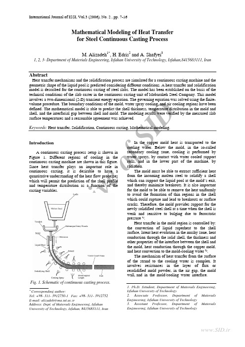
A rc hi v eo fSI DMathematical Modeling of Heat Transfer for Steel Continuous Casting ProcessM. Alizadeh 1*, H. Edris 2 and A. Shafyei 31, 2, 3- Department of Materials Engineering, Isfahan University of Technology, Isfahan,8415683111, IranAbstractHeat transfer mechanisms and the solidification process are simulated for a continuous casting machine and the geometric shape of the liquid pool is predicted considering different conditions. A heat transfer and solidification model is described for the continuous casting of steel slabs. The model has been established on the basis of the technical conditions of the slab caster in the continuous casting unit of Mobarakeh Steel Company. This model involves a two-dimensional (2-D) transient energy equation. The governing equation was solved using the finite-volume procedure. The boundary conditions of the mold, water spray cooling, and air cooling regions have been defined. The mathematical model is able to predict the shell thickness, temperature distribution in the mold and shell, and the interfacial gap between shell and mold. The modeling results were verified by the measured slab surface temperatures and a reasonable agreement was achieved.Keywords: Heat transfer, Solidification, Continuous casting, Mathematical modeling.IntroductionA continuous casting process setup is shown inFigure 1. Different regions of cooling in the continuous casting machine are shown in this figure.Since heat transfer plays an important role incontinuous casting, it is desirable to have aquantitative understanding of the heat flow processeswhich will permit the prediction of the shell profileand temperature distribution as a function of thecasting variables.Fig. 1. Schematic of continuous casting process.∗Corresponding author:Tel: +98- 311- 3912750-1 Fax: +98- 311- 3912752 E-mail: alizadeh@ma.iut.ac.irAddress: Dept. of Materials Engineering, Isfahan University of Technology, Isfahan, 8415683111, IranIn the copper mold heat is transported to the cooling water. Below the mold, in the so-called secondary cooling zone, cooling is performed by water sprays, by contact with water cooled supportrolls, and in the lower part of the machine, by radiation. The mold must be able to extract sufficient heat from the incoming molten steel to solidify a shell which can support the liquid pool at the mold’s exit, and thereby minimize breakouts. It is also important for the mold to be able to remove the heat uniformly to avoid the formation of thin regions in the shell which could rupture and lead to breakouts or surface cracks. Therefore, the mold provides support for the newly solidified steel shell at a time when the shell is weak and sensitive to bulging due to ferrostatic pressure 1).Heat transfer in the mold region is controlled by: the convection of liquid superheat to the shell surface, latent heat evolution in the mushy zone, heat conduction through the solid shell, the thickness and other properties of the interface between the shell and the mold, heat conduction through the copper mold, and heat convection to the mold-cooling water 2).The mechanism of heat transfer from the surface of the strand to the cooling water is complex. It involves resistances in the layer of flux or resolidified mold powder, in the air gap, the mold wall, and in the mold/cooling water interface.1. Ph.D. Sstudent, Department of Materials Engineering, Isfahan University of Technology2. Associate Professor, Department of Materials Engineering, Isfahan University of Technology3. Assistant Professor, Department of Materials Engineering, Isfahan University of TechnologyA rc hi v eo fSI DInternational Journal of ISSI, Vol.3 (2006), No. 2Table 1: Comparison of thermal conductivities of materials present in the continuous casting mold [3].MaterialsTemperature(o C) Thermal conductivity(W m -1 K -1)Steel St 37 1200 29 Copper 30-130 385 Casting flux 1000-1300 0.5 to 1.2 Water 25 0.62Radiation conductivity of gas gap 1000 0.043Fig. 2. Different regions and simulation domain in continuous casting process.The thermal conductivities of different layers are compared in Table 1. As shown in this table, the air gap has the largest resistance to heat flow, while the other parts have a comparatively small resistance. Therefore, the pattern of heat removal in the mold is dependent largely upon the dynamics of gap formation. The air gap or contact resistances can be generated by the shrinkage of the steel shell away from the mold walls, especially after the flux is completely solid and unable to flow into the gaps. More researches were performed to show that the air gap was usually created in the lowest one-third of the mold length 3).In the upper part of the secondary cooling zone, the strand is usually sprayed by water emerging from nozzles arranged in the spaces between the rolls. The rate at which heat is extracted from the strand surface by water sprays has been measured by many researchers. These researchers have shown that under normal continuous casting conditions, in which shell surface temperatures range between 700 and 1200 o C, surface temperature has a little effect on the heat transfer coefficient. All studies agree that, in the stated temperature range, the spray water flux has the most effect on the heat transfer coefficient. Moreover, the temperature of sprayed water does not have a large influence on the heat transfer coefficient 4).In the lower part of the secondary cooling zone, heat transfer is preferred mainly by radiation and by roll contact. Therefore, it should be considered that the oxide scales generated on the surface of the strand could cause a thermal resistance in this zone 5).In this study, the mathematical model has been established on the basis of the technical conditions of the slab caster in the continuous casting unit of Mobarakeh Steel Company. In this model, steel heat capacity and steel thermal conductivity were considered as functions of steel temperature and chemical composition. Considering these functions, the governing equation is a non-linear equation. In this study the equation is solved in non-linear state. This model is also capable of predicting the temperature distribution, including the solidus and liquidus isotherm which defines the solid shell and mushy zone, respectively, as a function of section size, pouring temperature, steel composition, casting speed, mold length and spray conditions.Mathematical modelingFigure 2 shows the different regions of the continuous casting machine and the model considered for physical simulation of the caster. A typical method of modeling the strand thermal condition is shown in this figure. The mathematical model is applied to slices of strand that start at the meniscus and travel through the machine at the casting speed. New slices are generated periodically. A sufficient number of slices exist in each cooling zone to give an accurate representation of the thermal condition in each zone. In this model, only a quarter of the strand is considered due to the symmetry of the heat flow conditions (Figure 3).A rc hi v eo fSI DInternational Journal of ISSI, Vol.3 (2006), No. 2Fig. 3. A symmetric quarter of strand width section with physical coordinate.AssumptionsThe following assumptions are made to simplify the mathematical model 6):-Conduction can take place only in the transverse directions.-Forced convective heat flow in the liquid pool is considered by defining an effective liquid thermal conductivity as:l eff K K ⋅=7(1) -The density of steel is constant, but specific heatcapacity and heat conductivity of steel are functions of temperature and chemical composition and therefore not constant.Model formulationThe energy conservation equation can be written as 7):(2)()()()()⎟⎠⎞⎜⎝⎛∂∂∂∂+⎟⎟⎠⎞⎜⎜⎝⎛∂∂∂∂+⎟⎠⎞⎜⎝⎛∂∂∂∂=∂∂+∂∂+∂∂+∂∂z T k z y T k y x T k x wH vH y uH x H t effeffeffρρρρ To simplify the equation, a transformation as wt z −=ζ is used. Therefore this is: (3)()ls ls s sH H H t y x H H q tHy H y x H x tH +==+∂∂−⎟⎟⎠⎞⎜⎜⎝⎛∂∂∂∂+⎟⎠⎞⎜⎝⎛∂∂∂∂=∂∂;,,,;0ζρααIn order to solve the governing equation, it is necessary to transform the physical domain into a computational domain. In general, this sort of transformation is used, and leads to a uniformly spaced grid in the computational domain but the points in physical domain may be unequally spaced. The original partial differential equation is transformed from physical coordinates (x, y ) to computational coordinates (ξ,η) by applying the chain rule of partial derivatives.;JS H H J H t x y s y x s s +⎟⎟⎠⎞⎜⎜⎝⎛∂∂∂∂+⎟⎟⎠⎞⎜⎜⎝⎛∂∂∂∂=⎟⎠⎞⎜⎝⎛∂∂ξηηαηηξξαξ (4);tH S l ∂∂−= y x J ηξ= In the above equations "S " is a term for heat source due to the metal phase transformation (liquid to solid). In order to establish the region of phase change, the latent heat contribution is specified as a function of temperature i.e. 8):f l l L f H ⋅=(5) Where L f is the latent heat of the phase changeand the liquid fraction (f l ) is computed by:⎪⎪⎭⎪⎪⎬⎫⎪⎪⎩⎪⎪⎨⎧≤≥≥−−≥=.......01sol sol liq sol liq sol liq l T T when T T T when T T T T T T when f (6)A typical 2D cartesian control volume is shownin Figure 4. This C.V contains a central node (P) with four neighborhood points (E, W, N, and S). The integral form of equation (4) is obtained on the control volume by the finite volume method 9,10): a P H sP = a E H sE + a W H sW + a N H sN + a S H sS + b (7) a P = a W + a E + a S + a N + a P oa E =ey x e ⎟⎟⎠⎞⎜⎜⎝⎛ΔΔηξξηα a W =wyx w ⎟⎟⎠⎞⎜⎜⎝⎛ΔΔηξξηα a N =nx y n ⎟⎟⎠⎞⎜⎜⎝⎛ΔΔξηηξα a S =sx ys ⎟⎟⎠⎞⎜⎜⎝⎛ΔΔξηηξαa P o =PJ t ⋅ΔΔ⋅Δηξ b = a P o (H sP o + H lP o - H lP ) + o Pq J ρηξΔ⋅Δ (8)Fig. 4. A typical control volume and the notation used for a Cartesian 2D grid [9].To approximate the variable values on the surface of the control volume, the Quadratic Upwind Interpolation (QUICK) algorithm is used 9). In the QUICK scheme, the variable profile between two points approximated by a parabola instead of aArc hi v eo fSI DInternational Journal of ISSI, Vol.3 (2006), No. 2straight line (Figure 5), on a uniform Cartesian grid leads to 9):W E P e φφφφ818386−+= (9)Fig. 5. Approximation of gradients at cell faces [9].Boundary conditionsTo solve the above equation, the boundary conditions are needed for different regions include the mold, water spray cooling, and air cooling. Figure 6 shows some machine cooling layouts while the technical information belonging to each zone is shown in Table 2. A general form of the boundary condition can be expressed through an equation (10), in which the heat transfer coefficient, h , is estimated for different cooling zones.()water b b T T h n T k −=∂∂−| (10)To determine the temperature of the boundaries, the discretion of the bnT |∂∂ on boundary points isrequired. According to the QUICK scheme b nT |∂∂could be calculated by the following correlation [10]: nT T T nT W P b bΔ+−=∂∂398(11)Therefore, as seen in equation (10), finding the heat transfer coefficient for different regions such as: mold, water spray, and air cooling is necessary.Fig. 6. Secondary cooling of the slab caster.In the mold, several thermal resistance layers exist between the steel shell surface and the recirculation water. All the thermal resistances in the mold are shown in Figure 7. The effective thermal resistance of the water channel is estimated from the water channel heat transfer coefficient, thermal conductivity and the thickness of scale deposits on the surface of the cooling-water channel 11):⎟⎟⎠⎞⎜⎜⎝⎛+=w scale scale water h k d r 1 (12)Fig. 7. Thermal resistances existing between the shell surface and water channel in the mold.Table 2. Secondary cooling zones variables.No. Zone Length zone(m)SegmentNumber of spray nozzles Water flow rate(m 3/sec)Number rollin zoneRoll radius (m)1 0.439 - -2 0.220 - -3 0.303 - 30 0.003975 - -4 0.925 0 38 0.004967 5 0.140 5 1.470 0 38 0.0048426 0.200 6 1.475 1 10 0.004858 5 0.2507 1.725 2 10 0.003975 5 0.3008 1.725 3 10 0.003733 5 0.3009 3.950 4,5 20 0.005667 10 0.350 10 5.200 Roll 37-47 22 0.006483 11 0.380,0.440 11 9.400 Roll 48-63 - Air cooling 16 0.440A rc hi v eo fSI DInternational Journal of ISSI, Vol.3 (2006), No. 2 The heat transfer coefficient between the water and the side walls of the water channel (h w ) is calculated assuming a turbulent flow through an equivalent-diameter pipe (D ) using the empirical correlation of Sleicher and Reusse 11):()21Pr Re 015.05c c water w Dkh += (13)()Pr 6.0215.0333.0;Pr 424.088.0−+=+−=e c cOther thermal resistances shown in Fig 7 can be calculated by the following correlations [11]:;;slag slag slag moldmold mold k d r k dr == ;air air air k d r = (14)Which d slag can be found from the powder consumption per mass of product (M slag (kg/ton)): ()N W N W M d slagsteel slag slag +×××=2ρρ (15) Also, d air includes a gap due to shrinkage of the steel shell, which can be calculated by the thermal linear expansion relation of steel using following correlation for each control volume: T l l Δ⋅⋅=Δλ (16) Where, λ is linear thermal expansion coefficient of steel and l is length of each control volume. Moreover, the heat transfer coefficient due to radiation is calculated by: ()()212221T T T T h rad ++=εσ (17) Heat transfer mechanisms in the spray cooling zones below the mold are defined in Figure 8. The heat extraction due to the water sprays is a function of the water flux. The relationship between the rate of heat extraction by the water sprays and the spray variables has been established in a number ofexperimental studies. One of the most widely usedrelations has been presented by Nozaki's 12): ();0075.013925.055.0water water spray T Q h ×−××= (18)Fig. 8. Heat transfer mechanisms in the secondarycooling zones [12].Due to the high temperature of the strand surfaceand the exposure of water to the surface, an oxidescale is produced on the surface of the strand. Despite the low thickness, the scale can have animportant role in the heat transfer control. Therefore,the effective heat transfer coefficient should be considered as 12):sprayscsceff h k h 11+=δ (19)It has already been mentioned that the cooling ofthe strand in the lower part of the secondary cooling zone is mainly done by radiation 12). Therefore, the equation for the heat transfer coefficient is given as follows:()().2.2am s am s rad T T T T h ++=εσ (20) Besides the radiation, heat transfer is alsoachieved by natural convections, but this part is rather small and can be neglected in comparison to radiation cooling.The symmetrical boundary condition has been considered for midplanes as follows:0.,00.,0=∂∂−==∂∂−=yTk y xTk x (21)Computation and verificationThe algebraic equation of the boundary conditions has been solved with a Tridiagonal Matrix Algorithm (TDMA) solver 13). As seen in equations(7) and (8), to solve the algebraic equation, it is necessary to know the latent enthalpy in a new time step (H l ). To update the amount of the latent enthalpy an iterative solution is used for each time step:11++−+=k sP k sP k lP k lP H H H H (22)As seen in the above equation, by using the sensitive enthalpy that has been obtained by solving the energy equation (H sP k+1), latent enthalpy could be updated in the k+1th inner iteration in each time stepto achieve a certain convergence. The calculation mentioned has been programmed in the FORTRAN language. The mathematic simulation starts by setting the initial steel temperature at the pouring temperature. Input parameters, in Table 3, in the standard cases are verified by the measured temperatures on the shell surface of the strand.Equilibrium lever-rule calculations are performed on a Fe-C phase diagram in order to calculate steel phase fractions. By this means, phase field lines are specified as simple linear functions of carbon equivalent content. The carbon of the steel is applied as the carbon equivalent content that is calculated by the following correlation 14): wt%CE=wt%C+0.04(wt%Mn)-0.14(wt%Si)-0.04(wt%Cr)-0.1(wt%Mo)-0.24(wt%Ti)+0.1(wt%Cu) For a 0.16%C, 1.3%Mn, 0.5%Si, 0.05%Cr, 0.03%Mo and 0.01%Ti plain carbon steel, the carbon equivalent percentage calculated as 0.135 and also the equilibrium phase diagram model calculates T liq.=1528 o C, T sol = 1494 o C. The solid fraction-A rc hi v eo fSI DInternational Journal of ISSI, Vol.3 (2006), No. 2temperature curve in the mushy zone obtained from the model is shown in Figure 9. As seen in this figure the relation between temperature and solid fraction of steel in the mushy zone is non-linear.Solidified shell thickness is one of the most important calculated parameters in the model, and the influence of the grid spacing on this parameter should be considered. The influence of the gridspacing on the solidified shell thickness, in exit point of the mold, is shown in Table 4. The thickness amounts in width and narrow sides are presented in this table. It is clear from Table 4 that when grid spacing is reduced, solidified thicknesses are changed and they are stable in a narrow limit with reduction of grid spacing lower than a certain limit. It can be concluded that the solidified shell thickness is independent of the mesh size with the reduction of grid spacing lower than a certain limit.The mold zone is a complex and important area in continuous casting machine. The solid shell growth in this zone is complicated and the results of this study are compared to those of some other researchers. The comparison between the results of the model in this study and experimentalmeasurement by some other researchers is shown in Figure 10. The figure shows the variation of growth of the solid shell thickness on the ingot for low carbon steel (0.06% C). It is clear that the results from numerical solution in this study have a very good compatibility with those of three 3-D model of Thomas and experimental measurement of Alberny and co-worker.Table 3. Input data for standard conditions.Carbon equivalent content, CE pct 0.132 pctSteel density, ρ7500 kg/m 3 Steel emissivity, ε0.8 Mold copper plates thickness 0.043×0.030 m ×m Total mold length 0.704 m Mold copper plates width 2.220×0.215 m ×m Scale thickness on the surface of mold cold face 0.00001 m Mold conductivity, k mold 315 W/mK Mold powder conductivity, k slag 1.27 W/mK Air conductivity, k air 0.083 W/mKMold powder density, ρslag0.650 kg/m 3 Mold powder consumption rate, M slag 0.8 kg/ton steel Casting speed, V c 0.0167 m/secPour temperature, T in 1546 oCLiquidus temperature, T liq. 1528.6 oCSolidus temperature, T sol. 1494 oC Working mold length 0.659 m Slab geometry, W ×N 1.250×0.203 m ×m Scale conductivity on the surface of slab, k sc 0.5 W/mK Scale conductivity on the surface of mold, k scale 1.0 W/mK Water channel geometry, large & small plates 25×5×29 & 22×5×26mm 3 Average cooling water temperature in the mold 28 oC Water flow rate entering the mold small plate, 0.0061 m 3/sec Water flow rate entering the mold large plate, 0.0553 m 3/sec Latent heat of the steel phase change, L f 272140 J/kgWater conductivity , k water0.615 W/mKSteel specific heat capacity [11], C p ()()()()⎪⎪⎪⎪⎪⎪⎭⎪⎪⎪⎪⎪⎪⎬⎫⎪⎪⎪⎪⎪⎪⎩⎪⎪⎪⎪⎪⎪⎨⎧≥=≤=≤+=≤=−==+=+=liqp liq sol p sol op p o p p op o p T T C T T T C T T C T C T C T C T C T C T C T C T C T C 7877721100*334.02681100850648850750*766.338497507001431700500*836.0268500*376.0456p p p p p p p p p p J/kgK Steel conductivity, k steelf l *k liq +(1-f l )*k sol W/mK Solid steel conductivity, k sol 33.0 W/mK Effective molten steel conductivity, k liq 7*43.0 W/mKScale thickness on the surface of slab , δsc0.001 mA rc hi v eo fSI DInternational Journal of ISSI, Vol.3 (2006), No. 2Table 4. Effect of mesh size on the shell thickness at mold exit.Grid system #nx ×n y Shell thickness at middle of wide face (m)Shell thickness at middle of narrow face (m)25×10 0.0145 0.0111 25×15 0.0135 0.0110 50×15 0.0136 0.0118 50×20 0.0133 0.0119 100×200.0136 0.0117 100×300.0131 0.0117Fig. 9. Phase fraction variation with temperature in mushy zone.Fig. 10. Comparison between model results and other references.Results and discussionThe calculated surface temperatures of a slab, for the Table 3 conditions as a function of the distance below the meniscus, are presented in Figure 11. This figure shows the calculated surface temperatures at the centers of the wide and narrow faces and at the corners of the slab caster. The central areas of the wide faces are cooled one-dimensionally, whereas the slab corners are subject to 2-D cooling. The slab corners can therefore become significantly colder than other parts of the inner wide face. At the beginning of straightening, the slab corner temperature is 230 o C less than the temperature at the center of the wide face. Control of corner cooling is critical for much of continuously cast products. The slab corners tend to have meniscus marks, which act as stress risers. A combination of temperature, stress risers and a low ductility region in the 700-900 o C temperature range during the straightening process often leads to cracks in the corners. One way to increase the corner temperature is to widen the strip of unsprayed strand at the corner. However, as the non-sprayed strip is widened, a hot spot will develop between the colder corner and the sprayed area. Thus, the design must be in a way to ensure that it does not cause other quality problems. Also, as seen in Figure 11, the intensity of heat transfer of mist spray cooling is less than cooling in the lower part of the mold for all of the curves, because of this, the model predicts a 200 o C reheating of the slab surfaceon leaving the mold. A similar situation also exists in water spray cooling and air cooling regions on the surface of the wide face slab.Fig. 11. Predicted surface temperature of strand. Figure 12 shows the solidified shell thickness profiles of both the narrow and wide faces of the slab. This figure shows a sudden change of slope at the beginning of the solidified shell growth curve. It is indicated that the rate of solidified shell growth is clearly high in the mold region. Figure 13 shows a set of data of the local heat flux density along the length of the mold [15]. There is a maximum of heat flux density somewhat below the meniscus. Downward, the heat flux density usually decreases. If the air gapA rc hi v eIDInternational Journal of ISSI, Vol.3 (2006), No. 2between the mold and strand approximately has uniform thickness, or it increases uniformly in the downward direction, the heat flux density along the length of the mold continuously decreases.Fig. 12. Predicted solidified shell thickness.Fig. 13. Heat flux density distribution along the length of the mold.Fig. 14. Effect of casting speed on the pool depth.The casting speed is the most effective parameter in changing the position of the solidified shell thickness profiles. The relation of the "metallurgical length" (maximum length of the liquid pool) with the casting speed is shown in Figure 14. Increase in casting speed decreases the holding time of the slab in the secondary cooling zones and increases the length of the liquid core. Therefore, casting speed is the most important factor in controlling mold heat extraction. The solidified shell thickness as a function of the casting speed of bothwide face and narrow face of the strand are shown in Figure 15. Since, a lower casting speed provides more time for the heat to be extracted from the shell, the shell thickness increases. Moreover, the shell thickness in the initial solidification stage decreases at the high casting speed, as shown in Figure 15, which often easily causes the breakout of strand. Therefore, to prevent this unfavorable defect, the casting speed is limited. It should be mentioned that steel composition and slab width in comparison to casting speed has no significant effect on the shell thickness. As seen in this figure, solidified shell thickness for wide face is higher than it is for narrow face. This is because of the different air gap sizes between mold powder and mold wall in both wide and narrow faces. The air gap size along the length of the mold is predicted by the model for both faces in Figure 16. As seen in this figure, total shrinkage value in narrow face is more than wide face as expected because width size of slab is much larger than thickness size in cross section of strand. Furthermore, this phenomenon could change Fig. 15. Effect of casting speed on shell thickness.Fig. 16. air gap size along the mold.Heat transfer in the mold is governed by these three resistances: the casting-mold interface, the mold wall, and the mold-cooling water interface. Although, thermal resistance due to the air gapA rc hi v e o fSI DInternational Journal of ISSI, Vol.3 (2006), No. 2 should also be considered while the amount of air gap thermal resistance is usually quite large compared to the other resistances especially for the lower portion of the mold. Temperatures of three points: slag layer/mold wall interface (T 1), mold wall (T 2), and water channel wall (T 3) as shown in Figure 7 are predicted by the model. Since, the heat flux for steady state conditions will be constant and independent of distance: (23)mold rad airradair slag s rad airrad air slags slags total water s r rr r r r T T rr r r r T T r T T r T T q +⎟⎟⎠⎞⎜⎜⎝⎛+⋅+−=⎟⎟⎠⎞⎜⎜⎝⎛+⋅+−=−=−=′321The above relation represents three equations for the three unknowns, T 1, T 2, and T 3. The results of the model predictions are shown in Figure 17(a) and Figure 17(b). As seen in these figures, the existence of the air gap between the shell surface and mold wall causes the T 1 to increase both in wide and narrow faces of strand. Since the air gap thickness in the narrow face is larger than the wide face, T 1 in the narrow face is much higher than in the wide face. Therefore, the pattern of heat removal in the mold is dependent largely upon the dynamics of gap formation. It causes temperature difference to exist in solidified shell and has a strong influence on transverse cracks generation in the mold region.Fig. 17. Predicted temperatures for T 1, T 2 and T 3 points in Fig 7 -(a) wide face and (b) narrow face (T 1=slag layer/mold wall interface temperature, T 2=mold wall temperature, and T 3=water channel wall temperature).The effect of the amount of superheat temperature of the molten steel, entering the mold, on the solidified shell thickness is shown in Figure 18. At first, with increasing the superheat temperature, the superheat flux will increase and therefore, the solidification rate decreases. This, in turn, reduces the thickness of the steel shell. On the other hand, by increasing the superheat temperature, the driving force for the heat transfer will increase. Therefore, as seen in Figure 18, the influence of the superheat temperature is insignificant to shell growth, especially in the wide face of the strand. Low superheat, near liquidus temperature, is beneficial to continuous casting. Internal quality is improved as the equated zone is made significantly larger. Therefore, a more desirable structure with greater resistance to halfway cracks is produced. Centerline segregation and porosity are also reduced or eliminated.Fig. 18. Effect of steel superheat temperature on the shell thickness at mold exit.Conclusions1- A finite volume heat transfer and solidification model has been formulated to predict the temperature field and liquid pool position in the continuous casting process under different conditions. This has been verified with the temperature measurement of slab surface.2- Casting speed is the most effective parameter on mold heat removal. Therefore, it is the most important factor in controlling solidified shell thickness and slab temperature.3- Since, the air gap size in narrow face of mold is higher than the wide face, the breakout of strand often occurs in the narrow face.4- Air gap existing in the casting-mold interface causes a large thermal resistance for heat transfer from the solidified shell to the mold. Therefore, it has a strong influence on product quality and casting problems, especially for the narrow face of strand. 5- High superheat temperature may cause breakouts at the mold exit, especially for the narrow face, so it should be exactly kept at a low level.。
多孔纤维织物热湿传递数值模拟的研究进展

多孔纤维织物热湿传递数值模拟的研究进展王红梅;郑振荣;张楠楠;张玉双;赵晓明【摘要】Research of numerical simulation of heat and moisture transfer can provide theoretical foundation for the preparation and heat⁃moisture properties evaluation of porous textiles. Based on the heat and moisture transfer mechanism, new progress of the heat and moisture transfer through fabrics was summarized in terms of heat and moisture transfer models, numerical simulation methods and test methods of fabricheat⁃moisture transport properties, and the problems existing in the numerical simulation of heat and moisture transfer in fabric were analyzed. Taking into consideration interweave structure characteristics of fabric and the physical properties of the yarn was proposed when coupled heat and moisture transfer model established in three⁃dimensionl. In addition, the change of material physical properties depending on practical application conditions was considered in the process of numerical analysis, heat and moisture transfer numerical model of fabric need further optimize and the improvement of the accuracy.%热湿传递数值模拟的研究可为多孔纤维织物的制备和热湿性能评估提供理论基础。
PO6016《湍流两相流动的模化与数值仿真》 课程教学大纲

2、掌握两相流的相似理论及模化方法,具备对两相流工程实际问题进行模 化设计与相似分析的能力。(A5.1、A5.4、B2、B4.1、B4.2)
的应用”和“基于数值仿真的热力新产品开发”,并开展课程陈述与讨论。通过面 向解决实际工程问题的课程实践,能够开拓学生的思路,教会他们运用理论知识 和科学的研究方法解决实际的科学技术问题,进行严格的科研训练和具备良好的 科研素质。
专题讲座 本课程将设置三次专业讲座,并通过工程案例分析具体讲解湍流两相流动的 模化方法和数值仿真技术,包括两相流模化方法、两相流数值仿真技术及其在工 程设计与产品开发中的应用。 四、考核与评估 课程得分比例如下:
1
课堂出席
10%
2
个人作业
15%
3 大作业(专题研究)
60%
4
课程陈述与讨论
15%
课堂出席 学生课堂出席成绩根据学生在课堂上的表现确定,包括出席、讨论、课堂练 习和表现等。评价课堂出席情况的标准包括参加者是否很好地倾听课程、能否积 极地参与课堂讨论、参加者的表达是否简洁和明确、能否有见地的分析案例和提 供清楚的论证。 个人作业 本课程在重点章节布置 4-6 次课后作业,主要是巩固已学基本概念和基本理 论,并运用基本知识解决关键问题,也推荐学生阅读经典的科技文献和综述。根 据作业完成情况和正确性评定成绩。 大作业(专题研究报告) 大作业(专题研究报告)是针对能源动力两相流工程实际问题开展专题研究,
出版商:
科学出版社
出版年:
1994
参考书目: Clement Kleinstreuer. Two-Phase Flow: Theory and Application, Taylor & Francis Group, New York, London, 2003 ISBN: 1-59169-000-5
超临界压力CO_2在垂直管内对流换热数值模拟
第43卷第3期原子能科学技术Vol.43,No.3 2009年3月Atomic Energy Science and TechnologyMar.2009超临界压力CO 2在垂直管内对流换热数值模拟李志辉,姜培学(清华大学热能工程系热科学与动力工程教育部重点实验室,北京 100084)摘要:对于超临界压力CO 2在垂直圆管(d in =2mm )内高进口雷诺数(Re =9000)条件下向上流动时的对流换热进行了数值模拟。
通过与实验数据进行对比来验证湍流模型的可靠性,并研究变物性和浮升力对壁面温度和湍动能的影响。
结果表明:在热流密度较高的情况下,向上流动时出现了局部换热恶化和换热强化现象,这主要归因于浮升力对湍动能分布的影响;采用LB 湍流模型能较好地模拟这种换热现象;在热流密度较低的情况下,未出现上述换热现象。
关键词:超临界压力;浮升力;换热恶化;数值模拟中图分类号:T K124 文献标志码:A 文章编号:100026931(2009)0320247205Numerical Simulation of Convection H eat T ransfer for CO 2at Supercritical Pressure in V ertical Circular TubeL I Zhi 2hui ,J IAN G Pei 2xue(Key L aboratory f or T hermal S cience and Pow er Engineering of M inist ry of Education ,De partment of T hermal Engineering ,Tsinghua Universit y ,B ei j ing 100084,China )Abstract : Convection heat t ransfer of CO 2at supercritical p ressure in a vertical circular t ube (d in =2mm )at high inlet Re (about 9000)was investigated numerically to analyze t he effect s of t he variatio n of t he p hysical p roperties and buoyancy on t he wall tempera 2t ure and t he t urbulent energy.The result s show t hat in t he case of high heat fluxes t he local heat t ransfer deterioration and enhancement during t he upward flow due to t he st rong influence of buoyancy result in change of t he t urbulent energy dist ribution.Simulations using t he LB t urbulence model correspo nd well wit h t he experimental data in upward flow.In t he case of low heat fluxes t he p henomenon of heat transfer deterioratio n or enhancement was not observed.K ey w ords :supercritical pressure ;buoyancy ;deterioration ;numerical simulation收稿日期:2007212201;修回日期:2008203220基金项目:教育部科学技术重大项目资助(306001);国家“863”计划资助项目(2006AA05Z416)作者简介:李志辉(1976—),男,山西晋城人,博士研究生,动力工程及工程热物理专业 从20世纪五、六十年代开始,国内外学者对超临界流体在管道中的对流换热已进行了大量的实验和理论研究[124]。
Mathematical Model for Fluid Flow and Heat Transfer in the Cooling Shaft of

Cpf Cp~ dp dh F ks K g h~f m n nx ny p qw q~ r r R0 RI S t t, ty Tf T~ uf Us ut vf vs v~ V Vf
general transport equation fluid specific heat, (J/(kg K)) solid specific heat, (J/(kg K)) particle diameter, (m) hydraulic diameter of the passage of gas flow, (m) inertial coefficient, dimensionless the coefficient of solid flow potential permeability, (mz) gravitational acceleration, -9.81, (m2/s) fluid-solid heat transfer coefficient, (W/(m 2 K)) mass flux through a control volume face unit outward normal vector the x -direction component of n the y -direction component of n fluid pressure, (Pa) heat flux at the wall, (W/m 2) source term the position vector radial coordinate, (m) the diameter of prechamber, (m) the diameter of the cooling chamber, (m) the surface area of cell face, (m2) unit vector tangential to the boundary. the x -direction component of t the y -direction component of t fluid temperature, (K) solid temperature, (K) Darcy velocity in x direction, (m/s) the coke descending velocity in x direction, (m/s) velocity vector component in t -direction Darcy velocity in r direction, (m/s) the coke descending velocity in r direction, (m/s) velocity vector component in n -direction, (m/s) velocity vector, (m/s) gas velocity vector, (m/s)
cfx计算共轭传热
cfx计算共轭传热英文回答:Conjugate heat transfer refers to the simultaneous transfer of heat between a solid body and a fluid medium. This phenomenon is commonly encountered in various engineering applications, such as cooling systems, heat exchangers, and combustion chambers. The understanding and analysis of conjugate heat transfer are crucial for designing efficient and reliable thermal systems.One approach to calculate conjugate heat transfer is by using the computational fluid dynamics (CFD) method. CFD is a numerical technique that solves the governing equations of fluid flow and heat transfer. In the case of conjugate heat transfer, the equations for fluid flow and heat transfer in the fluid domain and solid domain are coupled together.To perform a CFD simulation of conjugate heat transfer,the first step is to discretize the fluid and solid domains into smaller control volumes or finite elements. The governing equations, such as the Navier-Stokes equationsfor fluid flow and the heat conduction equation for solid, are then numerically solved within each control volume or finite element. The boundary conditions, such as the fluid velocity and temperature at the inlet and outlet, as wellas the solid surface temperature, need to be specified.The solution procedure involves iterating between the fluid and solid domains until convergence is achieved. In each iteration, the fluid properties, such as the density and viscosity, are updated based on the fluid temperature obtained from the previous iteration. The heat transfer between the fluid and solid is accounted for by considering the convective heat transfer coefficient and thetemperature difference between the fluid and solid surfaces.Conjugate heat transfer simulations can providevaluable insights into the heat transfer characteristicsand temperature distribution within a system. For example,in the design of a heat exchanger, the simulation resultscan help optimize the geometry and determine the required fluid flow rate to achieve the desired heat transfer rate. In a combustion chamber, the simulation can predict the temperature distribution on the solid walls and ensure that the materials can withstand the high temperatures.In addition to CFD, another approach to calculate conjugate heat transfer is through the use of analytical methods. Analytical solutions can be derived for simplified geometries and boundary conditions, allowing for a more straightforward and efficient calculation of heat transfer. However, analytical solutions are often limited toidealized scenarios and may not capture the complex flow and temperature patterns seen in real-world applications.In conclusion, conjugate heat transfer is a critical phenomenon in various engineering applications. The calculation of conjugate heat transfer can be performed using computational fluid dynamics or analytical methods. Both approaches have their advantages and limitations, and the choice of method depends on the specific problem and available resources.中文回答:共轭传热是指固体体和流体介质之间同时进行的热量传递。