图像处理_CMU Town06 Motion Image Dataset(CMU 城镇模型俯瞰图像数据集6)
德罗斯特

德罗斯特效应照片制作教程先说一下什么是德罗斯特效应,德罗斯特效应(Droste effect)是递归的一种视觉形式,是指一张图片的某个部分与整张图片相同,如此产生无限循环。
就好像是说,你拿着一面镜子,然后再站在一面镜子前面,让两面镜子相对。
你看到镜子里面的情景,是相同的,无限循环的。
德罗斯特效应是一组非常有意思的照片,非常神奇,有的需要你花时间去辨别,如果你在这些图像上盯着太久,你可能会觉得自己越来越走到框架里面,甚至造成头晕、胸闷、脑子混乱…这种神奇的效果就被称为“德罗斯特效应”。
开始之前我们需要3个软件,分别是photoshop,GIMP(类似于PS),还有一个名为Mathmap 的数学软件,作为插件性质嵌入到GIMP里面,就像PS里面的滤镜一样。
可以自己到网上搜索。
下载好之后就可以进行安装了1 解压2 将 mathmap.exe, libgsl.dll, libgslcblas.dll 复制到 GIMP 插件(plugin)目录,默认是C:\Program Files\GIMP 2\lib\gimp\2.0\plug-ins3 复制 mathmaprc 、new_template.c 到C:\Users\你的用户名\.gimp-2.8\mathmap如果没有mathmap这个文件夹的话请新建一个。
1 你需要一张事先准备好做效果的图片,并在photoshop里面将需要的框架部分抠出来,背景透明,并保存为PSD或PNG文件。
抠图,换背景,加投影,加灯光调色我就不一一介绍了2.把刚才做好的PSD文件拖到GIMP里面,选择菜单的 Filters/Generic/Mathmap/Mathmap 打开Mathmap 插件,如图3.在设置面板里(Settings)去掉自动预览项(Auto Preview)4.进入Expression界面,将原有的默认代码删除,粘贴上我给你们的代码(文章最后会补上),然后就可以点预览(Preview)按钮了5.切换到 User Variables 面板,勾选 Tile Based on Transparency 和 Transparency Points In 项,然后点左边的预览(Preview)按钮感谢代码for Mathmap的原作者Breic 和改进者Pisco Bandito附代码########################################## Droste Effect code for Mathmap #### Original Code by Breic (Ben) #### Adapted by Pisco Bandito (Josh) #### Version 4.0 #### This version for Windows and Linux ###########################################You may need to alter the values of the following 9 variables to suit your image. r1=.4; # r1 is the inner radius. r1 is greater than zero and less than r2r2=1; # r2 is the outer radius. r2 is greater than r1 and less than 1p1=1; # periodicity - the number of times the image will repeat per cyclep2=1; # number of strands - the number of "arms" the spiral will have# procedural scaling and rotationzoom=.1; #Between .1 and 10rotate=-30; #Between -360 and 360# Procedural ShiftingxShift=.2; #Between -1 and 1yShift=0; #Between -1 and 1### To avoid framing problems on the largest annulus when tiling based on transparency, look# outside (levelsToLookOut) levels to see if something farther out should cover up this pixel# Try setting to 0 to see framing errors; 1 should be sufficient unless you have three or more# image layers contributing to some pixel (in which case set it to 2 or more). Larger values# slow the code down, and may lead to floating point errors.##levelsToLookOut=3;########################################################################################################################## You should not have to change anything below this line ##########################################################################################################################imageX=W; # image size, in pixelsimageY=H;minDimension=min(imageX, imageY);## User Variables, set these on the User Settings Tab ##retwist=user_bool("Do Not Retwist (Leave Unchecked for Droste Effect)");retwist=!retwist;### Tiling can be based on transparency (if the input image is a tiff), or simply based on the# radius. Using transparency, there can be protrusions between different annular layers.# Tiling based on transparency, you can decide whether you want to look inward or # outward from a transparent pixel. For example, with a frame you'll want to look inward,# while for a flower you'll want to look outward.##tileBasedOnTransparency=user_bool("Tile Based on Transparency?"); transparentPointsIn=user_bool("Transparency Points In?");# Miscellaneous variablestrue=1;false=0;epsilon=.01;##Correct the Rotation Variablerotate=pi/180*rotate;### Droste-effect code starts here# Set Droste effect parameters##alpha=atan(p2/p1*log(r2/r1)/(2*pi));f=cos(alpha);beta=f*exp(I*alpha);# the angle of rotation between adjacent annular levelsif (p2 > 0)then angle = 2*pi*p1;elseangle =-2*pi*p1;end;### Code to set up the viewport properly##if (retwist) thenxbounds=[-r2,r2];ybounds=[-r2,r2];elseybounds=[0,2.1*pi];xbounds=[-log(r2/r1), log(r2/r1)];end;xymiddle=ri:[0.5*(xbounds[0]+xbounds[1]),0.5*(ybounds[0]+ybounds[1])];xyrange=xy:[xbounds[1]-xbounds[0], ybounds[1]-ybounds[0]];aspectRatio=W/H;xyrange[0]=xyrange[1]*aspectRatio;xbounds=[xymiddle[0]-0.5*xyrange[0],xymiddle[0]+0.5*xyrange[0]];z=ri:[(xbounds[0]+(xbounds[1]-xbounds[0])*(x+W/2)/W)+xShift,(ybounds[0]+(ybound s[1]-ybounds[0])*(y+H/2)/H)+yShift];if (retwist) then # only allow for procedural zooming/scaling in the standard coordinateszinitial=z;z=xymiddle+(z-xymiddle)/zoom*exp(-I*rotate);elsezinitial=r1*exp(z); # save these coordinates for drawing a frame laterzinitial=zinitial*zoom*exp(I*rotate);end;### The Droste effect math all takes place over the next six lines.# All the rest of the code is for niceties.##if (retwist) thenz2=log(z/r1);elsez2 = z;end;logz=z2; # save these coordinates for drawing a grid laterz=p1*z2/beta;rotatedscaledlogz=z; # save these coordinates for drawing a grid laterz=r1*exp(z);## End Droste effect math## Tilingif (tileBasedOnTransparency && levelsToLookOut > 0) thenif ( transparentPointsIn) then ratio=r1/r2*exp(-I*angle); end;if (!transparentPointsIn) then ratio=r2/r1*exp( I*angle); end;z=z*exp(levelsToLookOut*log(ratio));end;### When tiling based on transparency, color is accumulated into the colorSoFar variable,# while alphaRemaining tells how much remains for lower layers to contribute (initially 1,# finally 0).##colorSoFar=rgba:[0,0,0,0];alphaRemaining=1;ix=minDimension/2*z[0];iy=minDimension/2*z[1];color=origValXY(ix,iy);colorSoFar = colorSoFar + (color*(alpha(color)*alphaRemaining)); alphaRemaining=alphaRemaining*(1-alpha(color));# do we need to look inward from the current point, or outward?sign=0;if (tileBasedOnTransparency) thenif ( transparentPointsIn && alphaRemaining > epsilon) then sign=-1; end;if (!transparentPointsIn && alphaRemaining > epsilon) then sign= 1; end;elseradius=sqrt(z[0]*z[0]+z[1]*z[1]);if (radius < r1) then sign=-1; end;if (radius > r2) then sign= 1; end;end;if (sign < 0) then ratio=r2/r1*exp( I*angle); end;if (sign > 0) then ratio=r1/r2*exp(-I*angle); end;### Iteratively move inward or outward, until# the point has radius r in [r1, r2), if tileBasedOnTransparency=false# or until alphaRemaining=0, if tileBasedOnTransparency=true# In the latter case, we accumulate color at each step##iteration=0; maxiteration=10;while (sign != 0 && iteration < maxiteration) doz2=z*ratio;z=z2;rotatedscaledlogz=rotatedscaledlogz+ri:[0,-sign*angle];ix=minDimension/2*(z[0]);iy=minDimension/2*(z[1]);color=origValXY(ix,iy);colorSoFar = colorSoFar + (color*(alpha(color)*alphaRemaining));alphaRemaining=alphaRemaining*(1-alpha(color));radius=sqrt(z[0]*z[0]+z[1]*z[1]);sign=0;if (tileBasedOnTransparency) thenif ( transparentPointsIn && alphaRemaining > epsilon) then sign=-1; end;if (!transparentPointsIn && alphaRemaining > epsilon) then sign= 1; end;elseradius=sqrt(z[0]*z[0]+z[1]*z[1]);if (radius < r1) then sign=-1; end;if (radius > r2) then sign= 1; end;end;iteration=iteration+1;end;color=colorSoFar;color=rgba:[color[0], color[1], color[2], 1]; # set the alpha value to 1 (it could be <1 if the loop terminated at iteration maxiteration)#This last line is important, it returns the pixel value for the current pixel color。
grid_sample 原理
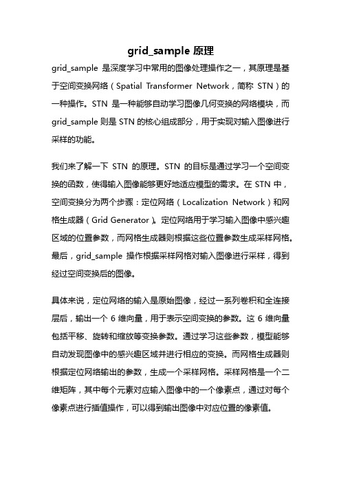
grid_sample 原理grid_sample是深度学习中常用的图像处理操作之一,其原理是基于空间变换网络(Spatial Transformer Network,简称STN)的一种操作。
STN是一种能够自动学习图像几何变换的网络模块,而grid_sample则是STN的核心组成部分,用于实现对输入图像进行采样的功能。
我们来了解一下STN的原理。
STN的目标是通过学习一个空间变换的函数,使得输入图像能够更好地适应模型的需求。
在STN中,空间变换分为两个步骤:定位网络(Localization Network)和网格生成器(Grid Generator)。
定位网络用于学习输入图像中感兴趣区域的位置参数,而网格生成器则根据这些位置参数生成采样网格。
最后,grid_sample操作根据采样网格对输入图像进行采样,得到经过空间变换后的图像。
具体来说,定位网络的输入是原始图像,经过一系列卷积和全连接层后,输出一个6维向量,用于表示空间变换的参数。
这6维向量包括平移、旋转和缩放等变换参数。
通过学习这些参数,模型能够自动发现图像中的感兴趣区域并进行相应的变换。
而网格生成器则根据定位网络输出的参数,生成一个采样网格。
采样网格是一个二维矩阵,其中每个元素对应输入图像中的一个像素点,通过对每个像素点进行插值操作,可以得到输出图像中对应位置的像素值。
接下来,我们详细介绍一下grid_sample操作的原理。
grid_sample操作的输入包括两个部分:输入图像和采样网格。
输入图像是一个四维张量,包括批次数、通道数、高度和宽度四个维度。
而采样网格是一个三维张量,包括批次数、高度和宽度三个维度。
grid_sample操作的输出也是一个四维张量,与输入图像具有相同的形状。
输出的每个像素点的值是通过对输入图像的插值操作得到的。
grid_sample操作的实现过程如下:首先,对于输出图像中的每个像素点,根据其在输出图像中的位置,通过采样网格找到对应的输入图像中的位置。
图像处理_CMU SRI Motion Image Dataset(CMU SRI运动图像数据集)

CMU SRI Motion Image Dataset(CMU SRI运动图像数据集)数据摘要:Taken with the Sony camera (borrowed from Stan Reifel) with the 12.5mm lens and the IR filter from the Fairchild head (which Bill took out for other reasons). The Sony camera has several advantages over the GE and the Fairchild.中文关键词:图像,索尼相机,通用电气,灵敏度,镜头,英文关键词:image,Sony camera,GE,sensitivity,lens,数据格式:IMAGE数据用途:图像处理,摄影技术数据详细介绍:SRI Motion Image DatasetTaken with the Sony camera (borrowed from Stan Reifel) with the 12.5mm lens and the IR filter from the Fairchild head (which Bill took out for other reasons). The Sony camera has several advantages over the GE and the Fairchild. It is inexpensive ($1000.). It appears to have none of the patterning I've seen in both the others (4 row and 4 column-type of "mesh" over the image). It has much better sensitivity than the Fairchild (I could barely see anything with the same lens and filter on the Fairchild.) It appears to have good blooming characteristics. The sunlight and flourescents don't cause it to bloom like the Fairchild.I took CAL0.IMG and CAL20.IMG via USR:[BOLLES]CALCAM.ICP, which takes one picture, moves the table 20" back from the target, and takes the second one.Using the formula of March 28 (page 3) I computed the following pixel sizes:1 horizontal pixel = .001170018"1 vertical pixel = .001089928"which would make the 256x240 (sampled down from 512x480) image plane to be.2995"(h) x .2616"(v). The specs say that the sensitive area on the chipis 8.8mm x 6.6mm or .3477" x .2596". I don't understand the differencein the horizontal sizes.Using this formula the two image plane distances corresponding to 30" onthe target were .1602925" and .1689388", which I believe should be the same, if the optics is symmetric, which it is. I don't know why there issuch a difference. (Maybe poor pointing accuracy of the cursor on the images ... only to the closest pixel.)I then used the 90" tape measured distance from the lens center to thetarget to get another estimate of the image plane distances. For a 30" target, the image plane distance should be 1/3 of F, which is .492126,which is .164042". Since that is a compromise between the two estimates from the first method I decided to use it and recompute the pixel sizes.The new sizes are:1 horizontal pixel = .001197387"1 vertical pixel = .001058336"However, this still does not account for the larger horizontal chip dimension. In pixels, 30" corresponds to 175 horizontal pixels and 201 vertical. If the aspect ratio is 4:3 so that 512 horiz pixels covers4 and 512 vert pixels covers 3, then one would think that the ratiowould be more like 150 H pixels and 200 V pixels for 30".These pixel sizes imply a field of view of 34.6 degrees H by 28.9 degrees V. Notice that the images were actually taken by shifting the table RIGHT.To correct for this their names will be redone sometime so that theyreally go right to left, which will confuse people if the clock canbe read ... It'll go backwards, Oh, well. See the ICP macro file SEQUENCE.ICP which was used to take the sequence ... it contains the cropping and resampling instructions ... basically 512x480 out of 512x512 and then sampled down to 256x240.The camera, instead of being horizontal, was tilted down slightly. We measured the tilt to be 7/32" over 2 & 5/8" which corresponds to an angleof 4.763642 degrees. At .001058336"/pixel this is an image plane distance of .0410105" or 38.75 pixels (out of 240 V pixels). Thus, the focusof expansion for AHTABLE pictures would be at (128,158) (starting with (0,0) vs (1,1)). To check this I took a horizontal picture (HORIZNTL.IMG) and marked the piercing point (256,240) in it and located that pointin AHTAB125.IMG. It was at (128,160), which agrees quite well with the number mentioned above. I then computed the angle that would place the focus of expansion at (128,160), which is 4.916568 degrees. I'll usethat as the pitch angle.Horizontal distances (vs. distances along the axis of the camera, whichis pointing down slightly) to some of the objects in the scene are:21.0 -- closest leg of the ladder21.5 -- the tip of the leaf at the top of the last image27.5 -- closest leaf at the bottom of the last image39.0 -- far leg of the ladder40.5 -- closest (upper left) corner of the shirt64.5 -- post near the middle of the picture68.0 -- lower left corner of the tilted wood backing for a light68.5 -- string holding the lead weight72.5 -- closest corner of the small box on the table72.5 -- label on the motor75.5 -- top right corner of tilted wood backing board79.0 -- closest side of the small conveyorbelt80.0 -- diagonal brace for the post (from top center to the left)91.5 -- top of the small vertical leaf of vertical plant on left95.5 -- pot holding that plant119.5 - the group of wires dropping down to the back of the terminals122.5 - upper right, closest corner of the keyboard100.0 - upper left corner on the back of the terminal148.5 - front of pot at the far end of the terminal table208.0 - front leg of the chair on the left224.5 - the back of the chair on the left277.0 - rightmost left of the cart, in the distance285.5 - leftmost pt on the black shade of the standing photo light295.5 - left visible left of the cart318.5 - left front side of the black cabinet on the right368.5 - far side of the tall cabinets on the left472.5 - front of the shelfs against the back wall491.5 - the clockThese distances were measured with a tape measure ... originally fromthe vise holding the camera and then subtracting 3.5" to the lens center.数据预览:点此下载完整数据集。
Single image motion deblurring using transparency

2. Previous Work
With unknown linear shift-invariant PSF [5], early approaches usually assume a priori knowledge to estimate the blur filter in deblurring the input image. In [2], with the defined parametric model, the values of the unknown parameters are estimated by inspecting the zero patterns in the Fourier transformation. The approaches proposed in [11, 12] model a blurred image as an autoregressive moving average (ARMA) process. The blur filter estimation is transformed to a problem of estimating the parameters of the ARMA process. Many methods solve the image deblurring using generalized cross-validation or maximum likelihood (ML) estimation. Expectation maximization (EM) is commonly adopted to maximize the log-likelihood of the parameter set. Kim et al. [9] restore the out-of-focus blurred image by estimating the filter in a parametric form. In [10, 19], recursive inverse filtering methods (RIF) are proposed to iteratively solve the image restoration problem. Extensive surveys on blind deconvolution can be found in [13, 6]. Recently, Fergus et al. [4] propose a variational Bayesian approach using an assumption on the statistical property of the image gradient distribution to approximate the unblurred image. An ensemble learning algorithm is employed which is originally proposed in [18] to solve the image separation problem. This method is proven effective in deblurring natural images and estimating complex blur filters. Image deblurring systems are also developed using hardware or multiple images to obtain more object structure and motion information in restoring degraded images. In [1], a high-resolution still image camera and a low-resolution video camera are connected where the low-resolution video camera is used to estimate the PSF. In [16], using fast im-
最新毕业设计-移动机器人的视觉的图像处理分析方法研究

毕业设计-移动机器人的视觉的图像处理分析方法研究移动机器人研究中的机器视觉研究正在兴起。
图像处理的丰富内容不仅提出了挑战,也为研究者提供了广阔的研究平台。
本文从移动机器人视觉系统入手,首先介绍了移动机器人视觉系统的概况和技术原理。
然后,依次阐述了移动机器人单目系统、双目系统和全景系统的基本原理,并举例说明了基于这三种视觉系统的图像处理方法。
其中,基于单目视觉的移动机器人SLAM方法结合CCD摄像机和里程计实现SLAM。
为了提高定位精度,避免错误定位的发生,在里程表定位的基础上,对不同视觉图像提取的特征进行匹配,根据极坐标几何计算摄像机的旋转角度,得到摄像机和里程表的角度冗余信息。
采用扩展卡尔曼滤波器(EKF)融合信息,提高了SLAM的鲁棒性。
针对基于双目视觉的移动机器人,针对立体视觉算法复杂度、且计算耗时的问题,提出了一种实时立体视觉系统的嵌入式实现方案,构建了一个以高性能多媒体数字信号处理器芯片TMS320DM642为核心的双通道视频采集系统。
使用高性能的数字信号处理器芯片可以满足实时性的要求,并且摆脱了以前由PC机实现的环境限制,如计算速度慢、功耗大等缺点。
为了解决室外机器人高精度定位问题,可以设计一种基于全景视觉近红外光源照度、全景视觉观测和手动编码路标的室外机器人定位系统。
该系统利用近红外成像减少光照和阴影的影响,利用全景视觉获取大范围的环境信息,依靠图像处理算法识别路标,最后利用三角测量算法完成机器人定位。
移动机器人在机器视觉方面的研究正在兴起,丰富的图像处理内容不仅给研究者带来了挑战,也为他们提供了一个广阔的平台这文本以机器人视觉系统.开始首先,介绍了移动机器人视觉系统的概况和技术原理然后描述了单目移动机器人系统、双目移动机器人系统和三眼移动机器人系统.的基本原理和它基于三个视觉系统.指定这些图像处理方法其中其中,基于单目视觉移动机器人的SLAM方法是CCD摄像机和里程计.的组合到提高定位精度,避免位置误差的发生,在里程表位置.的基础上,根据视觉图像的不同视角匹配各种特征我们可以根据极线几何计算摄像机旋转角度,利用里程计获取摄像机角度的冗余信息,并利用扩展卡尔曼滤波器(EKF).进行信息融合因此,这可以增强SLAM.的鲁棒性为基于双目视觉的移动机器人,立体视觉算法复杂,耗时等.我们可以通过嵌入系统.来呈现实时立体视觉计划它采用高性能多媒体芯片TMS320DM642作为双通道视频采集系统.这高性能DSP芯片.满足实时要求这方法摆脱了以往PC机的环境限制、计算速度慢、功耗大等缺点.为对于高精度室外机器人定位问题的要求,可以设计一个基于近红外光源照明、全景视觉观察和手动编码.的室外机器人定位系统这系统减少了近红外光图像对光线和阴影的影响,通过全景视觉系统获取大范围的环境信息,通过图像处理算法识别路标,并通过三角测量算法完成机器人的最终位置.介绍视觉是人类获取信息的最丰富的手段。
计算机视觉中的背景建模与运动目标检测技术

计算机视觉中的背景建模与运动目标检测技术计算机视觉是人工智能领域的一个重要分支,旨在使计算机具备理解和处理图像的能力。
在计算机视觉中,背景建模和运动目标检测是两个关键问题,它们能够帮助计算机自动识别图像中的目标物体和运动变化。
背景建模是指通过分析图像序列中的像素值,提取出背景信息并建立背景模型,从而实现对背景和前景的区分。
它是许多计算机视觉任务的基础,如运动目标检测、行人跟踪和视频分析等。
背景建模的关键问题是如何在不同光照条件下准确地估计背景模型,以便更好地检测运动目标。
传统的背景建模方法主要基于统计学模型,如高斯混合模型(GMM)和自适应背景平均(ABM)。
高斯混合模型假设每个像素的像素值是由一个或多个高斯分布组合而成,而自适应背景平均方法则通过对每个像素的像素值进行平均来建模。
然而,这些方法对于复杂场景的处理效果有限,比如光照变化、场景动态等。
近年来,随着深度学习的快速发展,基于深度学习的背景建模方法逐渐成为研究的热点。
深度学习模型能够自动提取图像的特征,并具有较强的非线性建模能力,可以更好地适应不同场景的复杂性。
例如,基于卷积神经网络(CNN)的背景建模方法,可以学习到图像的空间、时间和频率等多维特征,从而提高建模的准确性。
运动目标检测是计算机视觉中另一个重要的任务,它旨在自动检测和跟踪图像序列中的运动目标。
运动目标检测可以广泛应用于视频监控、交通流量统计、智能驾驶等领域。
基于背景建模的运动目标检测方法可以分为两类:基于像素的方法和基于区域的方法。
基于像素的方法主要通过将前景和背景进行像素级别的比较来实现目标的检测。
这类方法对光照变化和复杂背景的适应性较强,但对于噪声、遮挡和长时间运动等情况的处理效果较差。
相比之下,基于区域的方法则将图像分割成多个区域,并对每个区域进行运动目标的检测。
这类方法不仅可以提高检测的准确性,还可以减少计算量,但对于背景的变化较敏感。
随着计算机硬件的不断增强和图像处理算法的不断改进,背景建模和运动目标检测技术在实际应用中取得了令人瞩目的成果。
【CN110246094A】一种用于彩色图像超分辨率重建的6维嵌入的去噪自编码先验信息算法【专利】
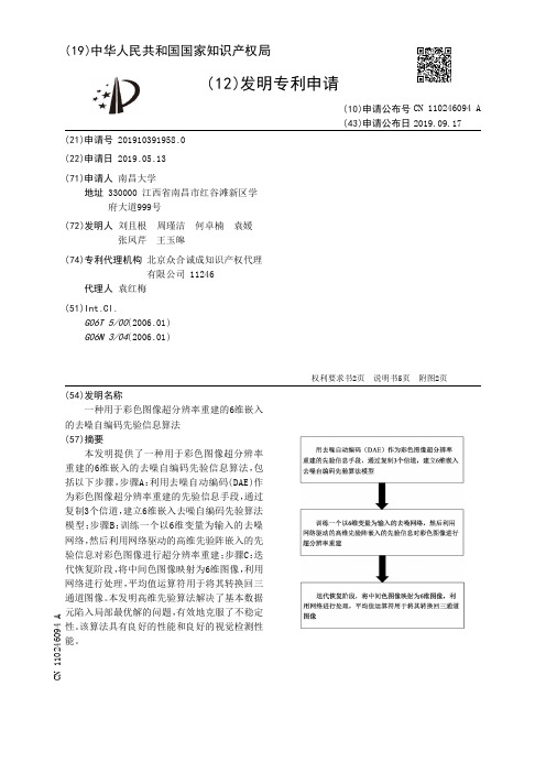
(19)中华人民共和国国家知识产权局(12)发明专利申请(10)申请公布号 (43)申请公布日 (21)申请号 201910391958.0(22)申请日 2019.05.13(71)申请人 南昌大学地址 330000 江西省南昌市红谷滩新区学府大道999号(72)发明人 刘且根 周瑾洁 何卓楠 袁媛 张凤芹 王玉皞 (74)专利代理机构 北京众合诚成知识产权代理有限公司 11246代理人 袁红梅(51)Int.Cl.G06T 5/00(2006.01)G06N 3/04(2006.01)(54)发明名称一种用于彩色图像超分辨率重建的6维嵌入的去噪自编码先验信息算法(57)摘要本发明提供了一种用于彩色图像超分辨率重建的6维嵌入的去噪自编码先验信息算法,包括以下步骤,步骤A:利用去噪自动编码(DAE)作为彩色图像超分辨率重建的先验信息手段,通过复制3个信道,建立6维嵌入去噪自编码先验算法模型;步骤B:训练一个以6维变量为输入的去噪网络,然后利用网络驱动的高维先验阵嵌入的先验信息对彩色图像进行超分辨率重建;步骤C:迭代恢复阶段,将中间色图像映射为6维图像,利用网络进行处理,平均值运算符用于将其转换回三通道图像。
本发明高维先验算法解决了基本数据元陷入局部最优解的问题,有效地克服了不稳定性。
该算法具有良好的性能和良好的视觉检测性能。
权利要求书2页 说明书5页 附图2页CN 110246094 A 2019.09.17C N 110246094A1.一种用于彩色图像超分辨率重建的6维嵌入的去噪自编码先验信息算法,其特征在于:包括以下步骤:步骤A:利用去噪自动编码(DAE)作为彩色图像超分辨率重建的先验信息手段,通过复制3个信道,建立6维嵌入去噪自编码先验算法模型;步骤B:训练一个以6维变量为输入的去噪网络,然后利用网络驱动的高维先验阵嵌入的先验信息对彩色图像进行超分辨率重建;步骤C:迭代恢复阶段,将中间色图像映射为6维图像,利用网络进行处理,平均值运算符用于将其转换回三通道图像。
图像处理_CMU Backyard Motion Image Dataset(CMU 后院场景运动图像数据集)

CMU Backyard Motion Image Dataset(CMU 后院场景运动图像数据集)数据摘要:The images were recorded on a umatic broadcast tape, and correspond to the even frames between time code 3:31:20 and 3:54:14 (about 23 seconds). They were taken with a hand-held Sony camcorder under overcast sky. Transferred to tape with a Sony BVU-920 videocassette player and a VIP matrox digitizer and frame buffer.中文关键词:运动,后院,校正器,移位,数字处理系统,英文关键词:motion,backyard,transfer,Digital Processing Systems,corrector,数据格式:IMAGE数据用途:图像处理,图像运动控制数据详细介绍:Backyard Motion Image DatasetDescriptionThe images were recorded on a umatic broadcast tape, and correspond to the even frames between time code 3:31:20 and 3:54:14 (about 23 seconds). They were taken with a hand-held Sony camcorder under overcast sky. Transferred to tape with a Sony BVU-920 videocassette player and a VIP matrox digitizer and frame buffer. A Digital Processing Systems timebase corrector was used during the transfer. Note that some images are obviously out of sequence, and probably many more.数据预览:点此下载完整数据集。