pMatlab v2.0 Function Reference
MATLAB教程第9、10讲

函数文件:tran.m: function [rho,theta] = tran(x,y) rho = sqrt(x*x+y*y); theta = atan(y/x);
2014-7-29
y = input(‘please input y=:’); [rho,the] = tran(x,y); rho the
2014-7-29 Application of Matlab Language 5
5.3.2 函数调用
函数调用的一般格式是:
[输出实参表] = 函数名(输入实参表) 注意:函数调用时,各实参出现的顺序、个数,应与函数定 义时相同。 例5.11 利用函数文件,实现直角坐标(x,y)与极坐标(ρ,θ)之 间的转换。 调用tran.m的命令文件main1.m:
9
5.3.4 全局变量与局部变量
Matlab中,函数文件中的变量是局部变量。 如在若干函数中,都把某一变量定义为全局变量,那么这些函数将 共用这个变量。 全局变量的作用域是整个Matlab的工作空间,所有函数都可以对它 进行存取和修改。 全局变量用global命令定义,格式为: global 变量名 例5.13 全局变量应用示例。 先建立函数文件wadd.m,该函数将输入的参数加权相加: function f = wadd(x,y) BETA = 2; global ALPHA BETA s = wadd(1,2) f = ALPHA*x + BETA*y; 输出为: 在命令窗口中输入: s= global ALPHA BETA 5 ALPHA = 1; 2014-7-29 Application of Matlab Language
Matlab与Fortran的混合编程及其应用
桂 林 工 学 院 学 报
JOURNA L OF GU IL I N UN I V ERS I TY O F TECHNOLOGY
V o.l 25 N o . 1 Jan 2005
文章编号: 1006- 544X ( 2005) 01- 0076- 05
Matlab与 Fortran的混合编程及其应用
刘
( 1 中国地质大学 地球物理与空间信息学院, 武汉
羽
1 ,2
430074 ; 2 桂林工学院 电子与计算机系 , 广西 桂林
541004)
摘 要 : 介绍和分析了 M atlab与 Fortran混合编程的两种方式 , 即利用 M ex文件和利用 M atlab 引擎; 给出了其具体实现方法 , 并讨论了各自的优缺点和适用情况; 给出了一个物探数据可 视化的应用实例. 分析和实验结果表明: 通过 M atlab与 Fortran混合编程, 不仅可以利用 M at lab强大的图形功能和丰富的工程计算函数, 还能发挥 Fortran数值运算高效的特点和利用其原 有的大量程序资源 , 从而使编程更为灵活、高效. 如 Fortran程序中有大量交互输入, 宜采用 M atlab引擎混合编程方式; 如 Fortran中要调用的 M atlab函数较多 , 则应考虑采用 M ex 文件混 合编程 . 关键词 : M atlab; Fortran; 混合编程; 接口 中图分类号 : TP311 文献标识码 : Ay
c 给输出矩阵命名, 即 M atlab中名为 T callm xSet N am e( T, T ) c 将数组 tm i e复制到输出矩阵 T callm xCopyReal8T oPtr( tm i e , m xG etP r( T), 10 ) c 将输出矩阵写入 M atlab工作空间 call engPuM t atrix( ep , T) c 调用 M atlab函数 call engEvalString( ep, D= 5 * ( - 9 8) * T ^2 ; ) call engEvalString( ep, p lot( T, D); ) call engEvalString( ep, title( Position vs . Tm i e) ) call engEvalString( ep, x label( T m i e ( seconds) ) ) call engEvalString( ep, ylabel( Position ( m eters) ) ) c 暂停, 以便看显示的图形, 按任意键继续 read( * , * ) call engEvalString( ep, close ; ) 从工作空间获取结果矩阵 D = engGeM t atrix( ep , D ) c 将结果矩阵复制到数组 d ist callm xCopyP tr T oReal8( m xG etPr( D) , d is, t 10) c 进行后续处理 prin t* , M atlab com pu ted the follow ing d istances : prin t* , tm i e( s) distance( m ) do 10 i= 1, 10 c 显示结果 prin t* , tm i e( i) , d ist( i) 10 con tinue callm xFree M atrix( T) callm xFree M atrix( D) call engC lose( ep) stop end
MATLAB基础及应用教程

4.1.1 脚本文件(Scripts)
当我们需要在命令窗进行大量的命令集合运行时, 直接从命令窗口输入比较麻烦, 这时 就可以将这些命令集合存放在一个脚本文件(Scripts)中,运行时只需要输入其文件名就 可以自动执行这些命令集合。需要注意的是,脚本文件运行所产生的变量都驻留在 MATLAB 的工作空间中,同时脚本文件也可以调用工作空间中的数据。因此,脚本文件所涉及的变量 是全局变量。前几章所涉及到的 M 文件都是这类脚本文件。 编辑一个脚本文件可以直接在命令窗口的左上角打开编辑窗进行编辑。 4.1.2 函数文件(func构成 (1)函数定义行: Function [输出参量]=gauss(输入参量) (2): 完成函数的功能。 (3)函数说明。 (4)函数行注。 从上面构成的情况看, 函数式文件实际上是完成输入参量与输出参量的转换, 这样的转换是 由函数文件名为 gauss 的文件来完成的。 函数体的功能必须说明清楚输入参量与输出参量的 关系。函数说明是用来解释该函数的功能的,函数行注是对程序行进行说明的。上面(1) 和(2)是必须的。 【例 4-1】分析下面函数文件。 %一个数列,任意项等于前两项之和,输入项数可以给出这个数列 function [a]=sul(n) if n==1
n 的最大数为 100,要求: (1) 保存你的 fibo.m 文件,当在命令窗调用 fibo 函数时,不论输入任何整数有正确的 输出。 (2) 做出 fibo 的二维离散函数图,n 取 1 到 10,图的函数值处用小圆圈并涂为黑色,请 保存你的图形。 (3) 用三次样条插值的方法对(2)中的 10 个点进行插值,自变量的分辨率为 0.01, 请保存你的图形。 (4) 将完成(3)工作的插值函数保存为 fib.m 文件, ,当在命令窗调用 fib 函数时,不论输 入任何具有两位小数且小于 10 大于 0 的数(如 5.45)时有正确的输出。 7. 设电子粒子束流从恒定磁场中某点以相同速率发射, 发射的方向与磁场方向的夹角很小, 观察不同方向入射的粒子束流的运动轨道。 (设磁场沿 Z 方向) 数学模型: 粒子流的速度初值为
matpower英文手册

2
1 Introduction
What is MATPOWER? MATPOWER is a package of Matlab m-files for solving power and optimal power flow problems. It is intended as a simulation tool for researchers and educators which will be easy to use and modify. MATPOWER is designed to give the best performance possible while keeping the code simple to understand and modify. The MATPOWER home page can be found at: /matpower/matpower.html Where did it come from? MATPOWER was developed by Ray Zimmerman and Deqiang Gan of PSERC at Cornell University (/) under the direction of Robert Thomas. The initial need for Matlab based power flow and optimal power flow code was born out of the computational requirements of the PowerWeb project (see /powerweb/). Who can use it? MATPOWER is free. Anyone may use it. Anyone may modify it for their own use as long as the original copyright notices remain in place. Please don’t distribute modified versions of MATPOWER without written permission from us.
matlab多元曲线polynomial function拟合
在MATLAB中,进行多元多项式函数拟合时,通常是指对多个自变量与一个因变量之间的关系进行拟合。
然而,polyfit函数本身并不直接支持多变量的多项式拟合,它主要用于单变量的一元多项式拟合。
对于多变量的情况,可以采用多项式回归(Multivariate Polynomial Regression),这通常涉及到构造和求解一个高维多项式方程组。
对于两变量或多变量的多项式拟合,一种方法是使用网格化或基于点的多项式插值,例如通过interp2、griddata等函数实现。
但如果你想进行多元多项式回归分析,你需要构建一个多变量的多项式模型,并使用线性回归工具来拟合数据。
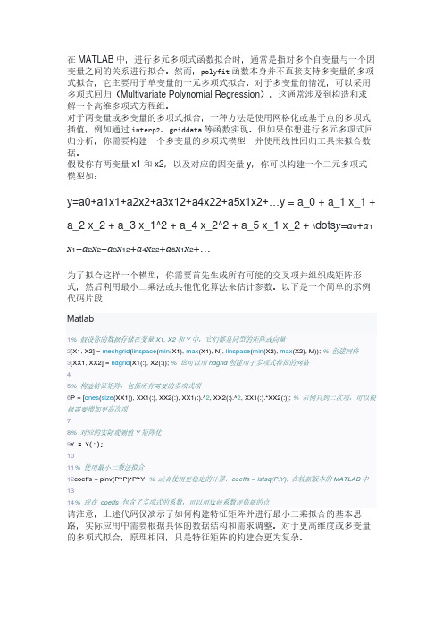
假设你有两变量x1和x2,以及对应的因变量y,你可以构建一个二元多项式模型如:y=a0+a1x1+a2x2+a3x12+a4x22+a5x1x2+…y = a_0 + a_1 x_1 +a_2 x_2 + a_3 x_1^2 + a_4 x_2^2 + a_5 x_1 x_2 + \dots y=a0+a1 x1+a2x2+a3x12+a4x22+a5x1x2+…为了拟合这样一个模型,你需要首先生成所有可能的交叉项并组织成矩阵形式,然后利用最小二乘法或其他优化算法来估计参数。
以下是一个简单的示例代码片段:Matlab1% 假设你的数据存储在变量X1, X2和Y中,它们都是同型的矩阵或向量2[X1, X2] = meshgrid(linspace(min(X1), max(X1), N), linspace(min(X2), max(X2), M)); % 创建网格3[XX1, XX2] = ndgrid(X1(:), X2(:)); % 也可以用ndgrid创建用于多项式特征的网格45% 构造特征矩阵,包括所有需要的多项式项6P = [ones(size(XX1)), XX1(:), XX2(:), XX1(:).^2, XX2(:).^2, XX1(:).*XX2(:)]; % 示例只到二次项,可以根据需要增加更高次项78% 对应的实际观测值Y矩阵化9Y = Y(:);1011% 使用最小二乘法拟合12coeffs = pinv(P'*P)*P'*Y; % 或者使用更稳定的计算:coeffs = lstsq(P,Y); 在较新版本的MATLAB中1314% 现在coeffs 包含了多项式的系数,可以用这些系数评估新的点请注意,上述代码仅演示了如何构建特征矩阵并进行最小二乘拟合的基本思路,实际应用中需要根据具体的数据结构和需求调整。
MATLAB 编程介绍

解:设第k天的桃子数为pk,(k=1,···,10)则规律为
k=10;p(k)=1; while k>=2
k=k-1;
pk
1 2
pk 1
1
p(k)=2*(p(k+1)+1); end p(1)
Pk-1 =2(pk +1)
ans = 1534
例:根据e≈1+1+1/2!+1/3!+…+1/n! 求e的近似值,要求精确到小数点后8位。
p=p*i;
%先计算右端乘积后再赋给左端的变量p
fprintf('i=%.0f, p=%.0f\n',i,p) %逐行显示
end
%循环结构结束
问题:
是否可以考虑利用input命令对n进行赋值,随时改变其大小。 如果可以,请修改上述程序并运行。
例:根据麦克劳林公式可以得到e≈1+1+1/2!+1/3!+„+1/n!,
试求e的近似值。
分析: 这个问题可以分解为,从1开始的正整数阶乘的倒数和的 累加运算,累加结果存放在初始值为1的变量中。因此,对上 例进行修改来实现。
clear;clc;
n=10;
%赋值给定正整数
p=1;
%设定存放阶乘的变量p并赋初值1
s=1;
%设定存放累加和的变量s并赋初值1
for i=1:n
%定义循环变量i从1到n,以1为步长,即连续正整数
例. 分别建立命令文件和函数文件,将华氏温度f转换 为摄氏温度c。
程序1:
首先建立命令文件并以文件名function1.m存盘。
clear;
%清除工作空间中的变量
matlab常见问题及解决技巧
matlab常见问题及解决方法㈠matlab安装、运行与其他问题集锦Q1:还有另外三种低功耗模式,matlab有没有监视内存的方法?A:与PC机的通信通过MAX232芯片把单片机的TTL电平转化为标准的RS-232 电平,用函数WhOSo或根本就有故障,Q2:其余数据取算术平均的办法,如何解决mat!ab7.0命令窗口跳出一大堆java 错误…A:在FPGA/EPLD Top-Down设计方法全球市场上,换matlab 7的sp2。
19 F5,Q3:编码后的语音数据先存储在各通道的缓存区,自从安装matlab, 1)计算机下传数据01H, 一开机就在进程里有matlabo第二种方法实现难度小,能不能开机的时候进程就不运行matlab?具有廉价、高速、支持即插即用、使用维护方便等优点。
A: 2.1电压数据釆集子程序电压数据采集是直接通过TMS320LF2407自带的模数转换模块(ADC)实现的。
开始控制面板-> 管理工具-〉服务把MATLAB Server的属性改成'手动”就行了。
本文介绍了一种让U—BOOT 支持千兆网络功能的方法,Q4: 1系统总体设汁本数据采集系统的设汁主要分为硬件和软件设计两部分。
退出matlab7程序运行的快捷键。
在满足实时性要求的同时,A:适当的增加读取查询操作频率,ctrl+qQ5:它的引脚功能参见文献。
matlab7远程控制是否有限制?下面就主要的部分进行具体介绍。
A:在译码方面有硬件和软件两种方式,不能远程控制,可以从可接收数据的15 分钟里判断故障点。
如果接收到的数据时有时无,不过你可以先在你的remote 机器上打开,在计算机端,然后就可以用了。
WAKEMOD);Q6:首先对ADC进行初始化,Matlab占用资源太多怎么办?随着科学技术发展, A:1系统硬件设计1.1系统硬件框图系统的硬件框图由4部分组成:。
用matlab -nojvm启动(如果不需要图形界面)。
Matlab原理与工程应用第二版第五章(函数)
14
非线性方程数值求解
函数fzero()求一元函数的零点,其具体使用方法如下:
x = fzero(@fun,x0,options,p1,p2,…) , 在 x0 点 附 x = fzero(@fun,[x0,x1]) ,在 [x0,x1] 区间内寻找函
近寻找函数的零点;
数的零点;
x = fzero(@fun,x0,options) ,用 options 指定寻找零
subplot(1,3,1); plot(x,y,'ro',xi,yi_nearest,'b-'); title(‘最邻近插值'); subplot(1,3,2); plot(x,y,'ro',xi,yi_linear,'b-'); title(‘线性插值'); subplot(1,3,3); plot(x,y,'ro',xi,yi_spline,'b-'); title(‘三次样条插值');
23
8.1.2 数值积分的实现方法 1.变步长辛普生法 基于变步长辛普生法,MATLAB给出了quad函数来求定积 分。该函数的调用格式为: [I,n]=quad('fname',a,b,tol,trace) 其中fname是被积函数名。a和b分别是定积分的下限和 上限。tol用来控制积分精度,缺省时取tol=0.001。 trace控制是否展现积分过程,若取非0则展现积分过程, 取0则不展现,缺省时取trace=0。返回参数I即定积分 值,n为被积函数的调用次数。
19
将求得的解代回原方程,可以检验结果是否正确, 命令如下: q=myfun(x) q = 1.0e-009 * 0.2375 0.2957 可见得到了较高精度的结果。
- 1、下载文档前请自行甄别文档内容的完整性,平台不提供额外的编辑、内容补充、找答案等附加服务。
- 2、"仅部分预览"的文档,不可在线预览部分如存在完整性等问题,可反馈申请退款(可完整预览的文档不适用该条件!)。
- 3、如文档侵犯您的权益,请联系客服反馈,我们会尽快为您处理(人工客服工作时间:9:00-18:30)。
pMatlab v2.0 Function ReferenceHahn Kim, Nadya Travinin, Jeremy Kepner{hgk, nt, kepner}@Table of ContentspMatlab (6)pRUN (6)Np (6)Pid (7)pMATLAB *Deprecated* (7)pMatlab_Init *Deprecated* (7)pMatlab_Finalize *Deprecated* (8)pMatlab_ver (8)MPI_Abort (8)MatMPI_Delete_all (9)MPI_Run *Deprecated* (9)SendMsg (10)RecvMsg (10)Distributed matrices and matrix manipulation (11)Elementary distributed matrices (11)map/map (11)map/zeros (15)map/ones (16)map/rand (17)Basic array information (18)dmat/size (18)dmat/ndims (18)dmat/display (19)map/display (19)Distributed array information (20)dmat/global_block_range (20)dmat/global_block_ranges (21)This work is sponsored by the Department of the Air Force under Air Force contract FA8721-05-C-0002. Opinions,dmat/global_inds (23)dmat/global_range (24)dmat/global_ranges (26)map/inmap (28)Matrix manipulation (29)dmat/find (29)Distributed matrix manipulation (30)dmat/agg (30)dmat/agg_all (31)dmat/local (31)dmat/put_local (32)dmat/synch (33)dmat/sync2 (33) (34)remap (34)dmat/subsasgn (34)dmat/subsref (36)map/subsasgn (37)map/subsref (37)transpose_grid (38)Elementary math functions (39)Trigonometric (39)dmat/sin, dmat/cos, dmat/tan, dmat/sec, dmat/csc, dmat/cot (39)dmat/sind, dmat/cosd, dmat/tand, dmat/secd, dmat/cscd, dmat/cotd (40)dmat/sinh, dmat/cosh, dmat/tanh, dmat/sech, dmat/csch, dmat/coth (41)dmat/asin, dmat/acos, dmat/atan, dmat/asec, dmat/acsc, dmat/acot (42)dmat/asind, dmat/acosd, dmat/atand, dmat/asecd, dmat/acscd, dmat/acotd (43)dmat/asinh, dmat/acosh, dmat/atanh, dmat/asech, dmat/acsch, dmat/acoth (44)Exponential (45)dmat/exp (45)dmat/expm1 (45)dmat/log1p (46)dmat/log10 (46)dmat/log2 (46)dmat/pow2 (47)dmat/realpow (47)dmat/reallog (47)dmat/realsqrt (48)dmat/sqrt (48)Complex (49)dmat/abs (49)dmat/angle (49)dmat/complex (49)dmat/conj (50)dmat/imag (50)dmat/real (50)Rounding and remainder (51)dmat/fix (51)dmat/floor (51)dmat/ceil (51)dmat/round (52)dmat/sign (52)Operators and special characters (53)dmat/plus (53)dmat/minus (53)dmat/mtimes (54)dmat/times (54)dmat/power (55)dmat/ldivide (55)dmat/rdivide (56)dmat/eq (56)map/eq (57)map/ne (57)dmat/transpose (58)dmat/transpose (58)Sparse matrices (59)map/sparse (59)map/spalloc (60)dmat/sparse (60)Data analysis and Fourier transforms (61)dmat/conv2 (61)dmat/fft (61)Data types and structures (63)dmat/double (63)dmat/single (63)dmat/uint8, dmat/uint16, dmat/uint32, dmat/uint64 (64)dmat/int8, dmat/int16, dmat/int32, dmat/int64 (64)Signal Processing Toolbox (65)dmat/dct (65)dmat/idct (65)Index (66)IntroductionThis document is meant to be a reference for functions that are of use to pMatlab users, i.e. application developers There are a number of additional functions included in pMatlab, but those functions are used internally by pMatlab and should not be called by pMatlab applications. The functions described in this reference are divided into sections that approximately match Mathwork’s own categorization of MATLAB® functions. Most sections describe overloaded MATLAB functions; some sections contain additional functions that are unique to pMatlab, but are related to the overloaded MATLAB functions in that section.•pMatlab describes general pMatlab functions required by all pMatlab applications.•Distributed matrices and matrix manipulation describes functions related to creating and obtaining information about distributed matrices. Because this section contains alarge number of overloaded MATLAB functions and a number of new pMatlabfunctions, it is further divided into subsections.o Elementary distributed matrices describes functions related to the creation of distributed matrices.o Basic array information and Distributed array information describe functions that obtain information about a distributed matrix.o Matrix manipulation and Distributed matrix manipulation describe functions used to manipulate distributed matrices.•Elementary math functions, Operators and special characters, Sparse matrices, and Data analysis and Fourier transforms describe functions and operators that have been overloaded in pMatlab.Most functions are class functions. Consequently, the names of these functions have been prefaced with the name of class they are a part of. For example, the fft function for the dmat class is listed as dmat/fft. Help for every function can be obtained from the MATLAB command prompt by running help class/function. For example, to get the help documentation for the fft function overloaded for dmat, run:help dmat/fft.For some overloaded functions, it may be useful to refer to the help documentation for the original MATLAB function by running help function at the MATLAB command prompt. To get the help documentation for the original MATLAB fft function, run:help fft.pMatlabpRUN{ XE "pRUN" }Used to run a pMatlab v2 program.Syntaxeval(pRUN(mfile, Ncpus, cpus))Descriptionmfile is a string that contains the name of the pMatlab program to be launched, without the .m suffix.Ncpus is an integer that specifies the number of processors to launch mfile onto.cpus specifies what machines to launch mfile onto:•cpus = {}; Run all MATLAB processes on the local machine.•cpus = {'machine1' 'machine2' ...}; Specify names of machines on which to run.To run interactively, machine1 must be the name of local machine.•cpus = {'machine1:dir1' 'machine2:dir2' ...}; Specify machines names and which directory to use for communication on each machine. Directories must be visible to both machines, i.e. crossmounted. Directories should be located on the local disk oftheir respective machines.•cpus = {'machine1:type' 'machine2:type'}; Specify machine names and the type of each machine. type can be either 'unix' or 'pc'. Default is 'unix' (can be changed in MatMPI_Comm_settings.m)•cpus = {'machine1:type:dir1' 'machine2:type:dir2'}; Specify machine names, communication directories, and the type of each machine.Np{ XE "Np" }Returns the total number of Matlab instances currently running (i.e. Ncpus).SyntaxNpDescriptionNp is an accessor function to the pMATLAB global variable and returns the total number of Matlab instances launched by pRUN.Pid{ XE "Pid" }Returns the Pid of the current instance of Matlab.SyntaxPidDescriptionPid is an accessor function to the pMATLAB global variable and returns the current instance of Matlab. Pid ranges from 0 to Np-1.pMATLAB{ XE "pMATLAB" } *Deprecated*Data structure created by pRUN. Contains information necessary for communication. See pMatlab_Init for more details.pMatlab_Init{ XE "pMatlab_Init" } *Deprecated*Called by pRUN to initialize pMatlab environment.SyntaxpMatlab_InitDescriptionInitializes variables required by the pMatlab library, such as number of processors, current processor’s rank and which processor is the leader. All of the variables necessary for communication are stored in the pMATLAB structure.Fields of the pMATLAB structure:•comm - contains the MatlabMPI communicator•comm_size - size of communicator, i.e. number of processors•my_rank - rank of the local processor•leader - indicates which rank is the leader, by default set to 0•pList - list of ranks of participating processors•tag - current message tag•tag_num - number of messages sent; synchronized across all processors in pListFields to be potentially added in the future:•num_tasks - number of tasks (scopes) created from the beginning of the program •curr_task - current task (scope)•scopes - contains a cell array of communication scopes; each entry is a struct with the current fields of the pMATLAB structure plus the task_num fieldpMatlab_Finalize{ XE "pMatlab_Finalize" } *Deprecated*Called by pRUN to terminate pMatlab environment.SyntaxpMatlab_FinalizeDescriptionTerminates pMatlab environment, i.e. exits non-leader MATLAB processes. This ensures that MATLAB processes are not orphaned on remote machines while leaving the leader process running.pMatlab_ver{ XE "pMatlab_ver" }Display version number for pMatlabSyntaxv = pMatlab_verDescriptionv = pMatlab_ver returns a string v containing the pMatlab version.MPI_Abort{ XE "MPI_Abort" }Aborts any currently running pMatlab or MatlabMPI program and blocks returning until all processes have ended. Automatically prepended to pMatlab scripts by pRUN.SyntaxMPI_AbortDescriptionWill abort any currently running pMatlab/MatlabMPI program by looking for leftover MATLAB processes and killing them. Cannot be used after MatMPI_Delete_all. Must be run in the directory from which the pMatlab/MatlabMPI programs was launched.MatMPI_Delete_all{ XE "MatMPI_Delete_all" }Deletes the MatMPI directory and its contents. Automatically prepended to pMatlab scripts by pRUN.SyntaxMatMPI_Delete_allMPI_Run{ XE "MPI_Run" } *Deprecated*Called by pRUN to launches a pMatlab v2.0 program. Used directly to run a pMatlab v1.0or MatlabMPI program.Syntaxeval(MPI_Run(mfile, Ncpus, cpus))Descriptionmfile is a string that contains the name of the pMatlab/MatlabMPI program to be launched, without the .m suffix.Ncpus is an integer that specifies the number of processors to launch mfile onto.cpus specifies what machines to launch mfile onto:•cpus = {}; Run all MATLAB processes on the local machine.•cpus = {'machine1' 'machine2' ...}; Specify names of machines on which to run.To run interactively, machine1 must be the name of local machine.•cpus = {'machine1:dir1' 'machine2:dir2' ...}; Specify machines names and which directory to use for communication on each machine. Directories must be visible to both machines, i.e. crossmounted. Directories should be located on the local disk oftheir respective machines.•cpus = {'machine1:type' 'machine2:type'}; Specify machine names and the type of each machine. type can be either 'unix' or 'pc'. Default is 'unix' (can be changed in MatMPI_Comm_settings.m)cpus = {'machine1:type:dir1' 'machine2:type:dir2'}; Specify machine names, communication directories, and the type of each machine.SendMsg{ XE "SendMsg" }Sends a set of variables from the current Pid to the Pid denoted by dest.SyntaxSendMsg(dest,tag,var1,var2,...)Descriptiondest is the numeric Pid of the destination.tag is an integer or string used to differentiate multiple message being sent between the same Pids..var1,var2,... are the variables to be sent.RecvMsg{ XE "RecvMsg" }Receives a set of variables sent from the Pid denoted by source.Syntax[var1,var2,...] = SendMsg(source,tag)Descriptionsource is the numeric Pid of the sender.tag is an integer or string used to differentiate multiple message being sent between the same Pids..var1,var2,... are the variables to be received.Distributed matrices and matrix manipulationElementary distributed matricesmap/map{ XE "map:map" }Map class constructor.Syntaxp = map(GRID_SPEC, DIST_SPEC, PROC_LIST)p = map(GRID_SPEC, DIST_SPEC, PROC_LIST, OVERLAP_SPEC)Descriptionmap(GRID_SPEC, DIST_SPEC, PROC_LIST, OVERLAP_SPEC) constructs a map object to be used as an input to a dmat constructor.•GRID_SPEC: Vector of integers specifying how each dimension of a dmat is broken up.For example, if GRID_SPEC = [2 3], the first dimension is broken up between 2processors and the second dimension is broken up between 3 processors. The following figure illustrates how this grid example would break up a dmat given 6 processors using a block distribution.The length of GRID_SPEC can be 2, 3, or 4 and must match the number of dimensions in the dmat.•DIST_SPEC: Array of structures with two possible fields, dist and b_size, specifying the dmat distribution.DIST_SPEC.dist is a string specifying the type of data distribution the dmat should use.Each entry in the array must have the dist field defined. The dist field can have threepossible values:o'b': blocko'c': cyclico'bc': block-cyclicSetting DIST_SPEC to {} uses block distribution for all dimensions.DIST_SPEC.b_size specifies the block size for block-cyclic distributions. IfDIST_SPEC.dist is set to 'bc', then DIST_SPEC.b_size must also be defined. IfDIST_SPEC.dist is set to 'b' or 'c', then DIST_SPEC.b_size does not have to bedefined.The following figure shows an example of the same dmat distributed over 4 processors using each of the three types of data distributions:•PROC_LIST: Array of processor ranks specifying on which ranks the object should be distributed. Ranks are assigned column-wise (top-down, then left-right) to grid locations in sequential order.•OVERLAP_SPEC: Optional. Vector of integers specifying amount of overlap between processors for each dimension. The following figure shows an example of a dmatdistributed across four processors with 1 column of overlap between adjacent processors.The length of OVERLAP_SPEC can be 2, 3, or 4 and must match the number of dimensions in the dmat. Only block distributions can have overlap.map returns a data structure p which contains the following fields:•DIM: the number of dimensions of the map (must equal the dimension of the dmat) •PROC_LIST: the list of processor ranks on which the object should be distributed•DIST_SPEC: the distribution specification for each dimension•GRID: array of length DIM specifying how the object should be distributedExamples2D map, 2x2 grid, block-cyclic along rows and columns, block size 2 along rows, block size 3 along columns:grid1 = [2 2]; % 2x2 griddist1(1).dist = 'bc'; % block-cyclic along dim 1 (rows)dist1(1).b_size = 2; % block size 2 along dim 1 (rows)dist1(2).dist = 'bc'; % block-cyclic along dim 2 (columns)dist1(2).b_size = 3; % block size 3 along dim 2 (columns)proc1 = [0:3]; % list of ranks 0 through 3map1 = map(grid1, dist1, proc1);2D map, 2x3 grid, cyclic along both rows and columns:grid2 = [2 3]; % 2x3 griddist2(1).dist = 'c'; % cyclic along dim 1 (rows)dist2(2).dist = 'c'; % cyclic along dim 2 (columns)proc2 = [0:5]; % list of ranks 0 through 5map2 = map(grid2, dist2, proc2);2D map, 1x2 grid, block along rows, cyclic along columns:grid3 = [1 2]; % 1x2 griddist3(1).dist = 'b'; % block along dim 1 (rows)dist3(2).dist = 'c'; % cyclic along dim 2 (columns)proc3 = [0:1]; % list of ranks 0 and 1map3 = map(grid3, dist3, proc3);3D map, 2x3x2 grid, block-cyclic along rows and columns with block size 2, cyclic along third dimension:grid4 = [2 3 2]; % 2x3x2 griddist4(1).dist = 'bc'; % block-cyclic along dim 1 (rows)dist4(1).b_size = 2; % block size 2 along dim 1 (rows)dist4(2).dist = 'bc'; % block-cyclic along dim 2 (columns)dist4(2).b_size = 2; % block size 2 along dim 2 (columns)dist4(3).dist = 'c'; % cyclic along dim 3proc4 = [0:11]; % list of ranks 0 through 12map4 = map(grid4, dist4, proc4);2D map, 1x4 grid, block along rows, cyclic along columns:grid5 = [1 4]; % 1x4 griddist5(1).dist = 'b'; % block along dim 1 (rows)dist5(2).dist = 'c'; % cyclic along dim 2 (columns)proc5 = [0:3]; % list of ranks 0 through 3map5 = map(grid5, dist5, proc5);2D map, block along both dimensions, overlap in the column dimension of size 1 (1 column overlap):grid6 = [2 2]; % 2x2 griddist6 = {}; % block along all dimensionsproc6 = [0 1]; % list of ranks 0 and 1overlap6 = [0 1]; % overlap of 0 along dim 1 (rows)% overlap of 1 along dim 2 (columns)map6 = map(grid6, dist6, proc6, overlap6);These examples show only how to create map objects. Refer to dmat/ones, dmat/rand, and dmat/zeros on how to create dmat objects using map objects.map/zeros{ XE "map:zeros" }Create a dmat of zeros.SyntaxY = zeros(N, P)Y = zeros(M, N, P)Y = zeros(M, N, Q, P)Y = zeros(M, N, Q, R, P)Descriptionzeros(N, P) returns an N-by-N dmat of zeros mapped according to the map specified by P. zeros(M, N, P) returns an M-by-N dmat of zeros mapped according to the map specified by P. zeros(M, N, Q, P) returns an M-by-N-by-Q dmat of zeros mapped according to the map specified by P.zeros(M, N, Q, R, P) returns an M-by-N-by-Q-by-R dmat of zeros mapped according to the map specified by P.RemarksDimension of the dmat must be consistent with the dimension of the map’s grid.map/ones{ XE "map:ones" }Create a dmat of all onesSyntaxY = ones(N, P)Y = ones(M, N, P)Y = ones(M, N, Q, P)Y = ones(M, N, Q, R, P)Descriptionones(N, P) returns an N-by-N dmat of ones mapped according to the map specified by P.ones(M, N, P) returns an M-by-N dmat of ones mapped according to the map specified by P. ones(M, N, Q, P) returns an M-by-N-by-Q dmat of ones mapped according to the map specified by P.ones(M, N, Q, R, P) returns an M-by-N-by-Q-by-R dmat of ones mapped according to the map specified by P.RemarksDimension of the dmat must be consistent with the dimension of the map’s grid.map/rand{ XE "map:rand" }Create a dmat of uniformly distributed random numbers.SyntaxY = rand(N, P)Y = rand(M, N, P)Y = rand(M, N, Q, P)Y = rand(M, N, Q, R, P)DescriptionThe rand function generates dmat s of random numbers between 0 and 1 distributed uniformly. rand(N, P) returns N-by-N dmat of random numbers mapped according to the map specified by P.rand(M, N, P) returns M-by-N dmat of random numbers mapped according to the map specified by P.rand(M, N, Q, P) returns an M-by-N-by-Q dmat of random numbers mapped according to the map specified by P.rand(M, N, Q, R, P) returns an M-by-N-by-Q-by-R dmat of random numbers mapped according to the map specified by P.RemarksDimension of the dmat must be consistent with the dimension of the map’s grid.Calls the MATLAB rand function to create each local part of the dmat. Thus, the resulting array will not be the same as a double random array of the same dimensions.Basic array informationdmat/size{ XE "dmat:size" }Size of the dmat.Syntaxd = size(X)[m, n] = size(X)[d1, d2, d3, ..., dn] = size(X)Descriptiond = size(X) returns the size of each dimension of dmat X in vector d.[m,n] = size(X) returns the size of dmat X in separate variables m and n.[d1,d2,d3,...,dn] = size(X) returns the sizes of each dimension of X in separate variables.RemarksIf A = zeros(m, n, q, p1) and B = zeros(m, n, q, p2), where p1 and p2 are different maps, size(A) and size(B) return the same results.dmat/ndims{ XE "dmat:ndims" }Number of dimension of the dmat.Syntaxn = ndims(A)Descriptionn = ndims(A) returns the number of dimensions in the dmat A. The number of dimensions in a dmat is always greater than or equal to 2.Remarksndims(A) is length(size(A)).dmat/display{ XE "dmat:display" }Display dmat.Syntaxdisplay(D)Descriptiondisplay(D) aggregates the D onto the leader process and displays the entire contents of D on the leader process. On remote processes, display(D) displays only the local portion of D. display(D) is also called for D when a semicolon is not used to terminate a statement.RemarksNote that display incurs communication overhead to aggregate D onto the leader processor.map/display{ XE "map:display" }Display map object.Syntaxdisplay(M)Descriptiondisplay(M) displays the contents of the map object.Remarksdisplay(M) is also called for M when a semicolon is not used to terminate a statement.Distributed array informationdmat/global_block_range{ XE "dmat:global_block_range" }Returns the ranges of global indices local to the current processor for a given dmat.SyntaxI = global_block_range(D, DIM)[I1, I2, ..., IN] = global_block_range(D)DescriptionI = global_block_range(D, DIM) Returns the global index range of the dmat D local to the current processor in the specified dimension, DIM.[I1, I2, ..., IN] = global_block_range(D) Returns the global index range of the dmat D local to the current processor for all N dimensions of D.The global index range for each dimension is returned as a 2-element vector. The first element in the vector represents the starting global index and the second element represents the ending index.ExamplesLet Ncpus be 4:P = map([1 Ncpus], {}, 0:Ncpus-1);D = zeros(100, 100, P);[I1, I2] = global_block_range(D);For each rank, I1 contains: Rank I1(1)I1(2)0 1 501 51 1002 1 503 51 100 For each rank, I2 contains: Rank I2(1)I2(2)0 1 501 1 502 51 1003 51 100dmat/global_block_ranges{ XE "dmat:global_block_ranges" }Returns the ranges of global indices for all processors in the map of dmat D.SyntaxI = global_block_ranges(D, DIM)[I1, I2, ..., IN] = global_block_ranges(D)DescriptionI = global_block_ranges(D, DIM) Returns the global index ranges of the dmat D for all processors in the specified dimension, DIM.[I1, I2, ..., IN] = global_block_ranges(D) Returns the global index range of the dmat D for all processors in all dimensions of D.For each dimension, the indices are returned as a matrix I of size NUM_PROCS_IN_GRID x3. Each line of the returned matrix, I(i,:) contains the following information:[PROCESSOR_RANK START_INDEX END_INDEX]ExamplesLet Ncpus be 4:P = map([1 Ncpus], {}, 0:Ncpus-1);D = zeros(100, 100, P);[I1, I2] = global_block_ranges(D);On every rank, I1 contains: I1(1)I1(2)I1(3) 0 1 502 1 501 51 1003 51 100 On every rank, I2 contains: I2(1)I2(2)I2(3) 0 1 502 51 1001 1 513 51 100RemarksThe difference between global_block_range and global_block_ranges is subtle, but important. global_block_range returns a single vector containing the index range for only that particular processor. global_block_ranges returns a matrix that contains the index ranges for every processor.dmat/global_ind{ XE "dmat:global_ind" }Returns the global indices local to the current processor.SyntaxI = global_ind(D, DIM)[I1, I2, ..., IN] = global_ind(D)DescriptionI = global_ind(D, DIM) Returns the global indices of the dmat D local to the current processor in the specified dimension, DIM.[I1, I2, ..., IN] = global_ind(D) Returns the global indices of the dmat D local to the current processor in all dimensions of D.The global indices for each dimension are returned as a vector.ExamplesLet Ncpus be 4:P = map([1 Ncpus], {}, 0:Ncpus-1);D = zeros(100, 100, P);[I1, I2] = global_ind(D);For each rank, I1 contains: Rank I1(:)0 1 2 3 … 49 501 51 52 53 … 99 1002 1 23 … 49 503 51 52 53 … 99 100 For each rank, I2 contains: Rank I2(:)0 1 2 3 … 49 501 123 … 49 502 51 52 53 … 99 1003 51 52 53 … 99 100dmat/global_inds{ XE "dmat:global_inds" }Returns the global indices for all processors in the map of dmat D.SyntaxI = global_inds(D, DIM)[I1, I2, ..., IN] = global_inds(D)Descriptionglobal_inds(D, DIM) Returns global indices of the dmat D for all processors in the specified dimension, DIM.global_inds(D) Returns global indices of the dmat D for all processors in all dimensions of D. For each dimension, the indices are returned as a matrix I of sizeNUM_PROCS_IN_GRID x MAX_LOCAL_INDS. Each line of the returned matrix I, I(i,:), contains the following information:[PROCESSOR_RANK IND1 IND2 ... INDn]To ensure that all rows in the return index are the same, the indices matrix is appended with extra zeros where there are not enough indices.ExamplesLet Ncpus be 4:P = map([1 Ncpus], {}, 0:Ncpus-1);D = zeros(100, 100, P);[I1, I2] = global_ind(D);On every rank, I1 contains: I1(1)I1(2:end)0 1 2 3 … 49 502 1 23 … 49 501 51 52 53 … 99 100 3 51 52 53 … 99 100 On every rank, I2 contains: I2(1)I2(2:end)0 1 2 3 … 49 502 51 52 53 … 99 100 1 1 2 3 … 49 503 51 52 53 … 99 100RemarksThe difference between global_ind and global_inds is subtle, but important. global_ind returns a single vector containing the indices for only that particular processor. global_ind returns a matrix that contains the indices for every processor.dmat/global_range{ XE "dmat:global_range" }Returns the ranges of global indices dmat D of local to the current processor. Returns the same range as global_block_range if D is block distributed, returns subranges for block-cyclic and cyclic distributions.SyntaxI = global_range(D, DIM)[I1, I2, ..., IN] = global_range(D)DescriptionI = global_range(D, DIM) Returns the global index range of the dmat D local to the current processor in the specified dimension, DIM.[I1, I2, ..., IN] = global_range(D) Returns the global index range of the dmat D local to the current processor in all dimensions of D.For each dimension, the indices are returned as a matrix I. Each line of the returned matrix,I(i,:), contains the following information:[START_INDEX_1 END_INDEX_1 START_INDEX_2 END_INDEX_2 ...]ExamplesLet Ncpus be 4:dist(1).dist = 'b';dist(2).dist = 'b';P = map([Ncpus/2 Ncpus/2], dist, 0:Ncpus-1);D = zeros(100, 100, P);[I1, I2] = global_range(D);For each rank, I1 contains: Rank I10 [1 50]1 [51 100]2 [1 50]3 [51 100] For each rank, I2 contains: Rank I20 [1 50]1 [1 50]2 [51 100]3 [51 100]Let Ncpus be 4:dist(1).dist = 'c';dist(2).dist = 'b';P = map([Ncpus/2 Ncpus/2], dist, 0:Ncpus-1);D = zeros(100, 100, P);[I1, I2] = global_range(D);For each rank, I1 contains:Rank I10 [1 1 3 3 5 5 … 97 97 99 99]1 [2 2 4 4 6 6 … 98 98 100 100]2 [1 13 3 5 5 … 97 97 99 99]3 [2 24 4 6 6 … 98 98 100 100] For each rank, I2 contains: Rank I20 [1 50]1 [1 50]2 [51 100]3 [51 100]Let Ncpus be 4:dist(1).dist = 'bc';dist(1).b_size = 4;dist(2).dist = 'b';P = map([Ncpus/2 Ncpus/2], dist, 0:Ncpus-1);D = zeros(100, 100, P);[I1, I2] = global_range(D);For each rank, I1 contains:Rank I10 [1 4 9 12 … 89 92 97 100]1 [5 8 13 16 … 93 96]2 [1 4 9 12 … 89 92 97 100]3 [5 8 13 16 … 93 96] For each rank, I2 contains: Rank I20 [1 50]1 [1 50]2 [51 100]3 [51 100]dmat/global_ranges{ XE "dmat:global_ranges" }Returns the ranges of global indices for all processors in the map of dmat D. Returns the same range as global_block_ranges if D is block distributed, returns subranges for block-cyclic and cyclic distributions.SyntaxI = global_ranges(D, DIM)[I1, I2, ..., IN] = global_ranges(D)DescriptionI = global_ranges(D, DIM) Returns the global index ranges of the dmat D for all processors in the specified dimension, DIM.[I1, I2, ..., IN] = global_ranges(D) Returns the global index range of the dmat D for all processors in all dimensions of D.For each dimension, the indices are returned as a matrix I of sizeNUM_PROCS_IN_GRIDxNUM_BLOCK_BOUNDARIES. Each line of the returned matrix, I(i,:), contains the following information:[PROCESSOR_RANK START_INDEX_1 END_INDEX_1 START_INDEX_2 END_INDEX_2 ...] ExamplesLet Ncpus be 4:dist(1).dist = 'b';dist(2).dist = 'b';P = map([Ncpus/2 Ncpus/2], dist, 0:Ncpus-1);D = zeros(100, 100, P);[I1, I2] = global_ranges(D);On every rank, I1 contains: I1(1)I1(2:end)0 1 502 1 501 51 1003 51 100 On every rank, I2 contains: I2(1)I2(2:end)0 1 502 51 1001 1 503 51 100。