2The coordination generalized particle model—An evolutionary approach to multi-sensor fusion

合集下载

一些英文审稿意见的模板

最近在审一篇英文稿，第一次做这个工作，还有点不知如何表达。

幸亏遇上我的处女审稿，我想不会枪毙它的，给他一个major revision后接收吧。

呵呵网上找来一些零碎的资料参考参考。

+++++++++++++++++++++++++++++++1、目标和结果不清晰。

It is noted that your manuscript needs careful editing by someone with expertise in technical English editing paying particular attention to English grammar, spelling, and sentence structure so that the goals and results of the study are clear to the reader.2、未解释研究方法或解释不充分。

In general, there is a lack of explanation of replicates and statistical methods used in the study.Furthermore, an explanation of why the authors did these various experiments should be provided.3、对于研究设计的rationale:Also, there are few explanations of the rationale for the study design.4、夸张地陈述结论/夸大成果/不严谨：The conclusions are overstated. For example, the study did not showif the side effects from initial copper burst can be avoid with the polymer formulation.5、对hypothesis的清晰界定：A hypothesis needs to be presented。

Measurement of the Cross-Section for the Process Gamma-Gamma to Proton-Antiproton at sqrt(s

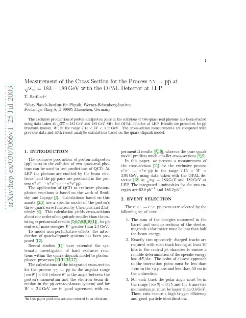
a r X i v :h e p -e x /0307066v 125 J u l 20031Measurement of the Cross-Section for the Process γγ→p¯p at √s ee =183GeV and 189GeV with the OPAL detector at LEP.Results are presented for p¯pinvariant masses,W ,in the range 2.15<W <3.95GeV.The cross-section measurements are compared with previous data and with recent analytic calculations based on the quark-diquark model.1.INTRODUCTIONThe exclusive production of proton-antiproton (p¯p )pairs in the collision of two quasi-real pho-tons can be used to test predictions of QCD.At LEP the photons are emitted by the beam elec-trons 1and the p¯p pairs are produced in the pro-cess e +e −→e +e −γγ→e +e −p¯p .The application of QCD to exclusive photon-photon reactions is based on the work of Brod-sky and Lepage [1].Calculations based on this ansatz [2,3]use a speciﬁc model of the proton’s three-quark wave function by Chernyak and Zhit-nitsky [4].This calculation yields cross-sections about one order of magnitude smaller than the ex-isting experimental results [5,6,7,8,9,10,11],for p¯p centre-of-mass energies W greater than 2.5GeV.To model non-perturbative eﬀects,the intro-duction of quark-diquark systems has been pro-posed [12].Recent studies [13]have extended the sys-tematic investigation of hard exclusive reac-tions within the quark-diquark model to photon-photon processes [14,15,16,17].The calculations of the integrated cross-section for the process γγ→p¯p in the angular range|cos θ∗|<0.6(where θ∗is the angle between the proton’s momentum and the electron beam di-rection in the p¯p centre-of-mass system)and for W >2.5GeV are in good agreement with ex-s ee =183GeV and 189GeV atLEP.The integrated luminosities for the two en-ergies are 62.8pb −1and 186.2pb −1.2.EVENT SELECTIONThe e +e −→e +e −p¯p events are selected by the following set of cuts:1.The sum of the energies measured in the barrel and endcap sections of the electro-magnetic calorimeter must be less than half the beam energy.2.Exactly two oppositely charged tracks are required with each track having at least 20hits in the central jet chamber to ensure a reliable determination of the speciﬁc energy loss d E/d x .The point of closest approach to the interaction point must be less than 1cm in the rφplane and less than 50cm in the z direction.3.For each track the polar angle must be in the range |cos θ|<0.75and the transverse momentum p ⊥must be larger than 0.4GeV.These cuts ensure a high trigger eﬃciency and good particle identiﬁcation.24.The invariant mass W of the p¯p ﬁnal state must be in the range 2.15<W <3.95GeV.The invariant mass is determined from the measured momenta of the two tracks using the proton mass.5.The events are boosted into the rest system of the measured p¯p ﬁnal state.The scatter-ing angle of the tracks in this system has to satisfy |cos θ∗|<0.6.6.All eventsmustfulﬁl the trigger conditions described in [11].7.The large background from other exclusive processes,mainly the production of e +e −,µ+µ−,and π+π−pairs,is reduced by par-ticle identiﬁcation using the speciﬁc energy loss d E/d x in the jet chamber and the energy in the electromagnetic calorimeter.The d E/d x probabilities of the tracks must be consistent with the p ands ee =183GeV and 128events at√d W d |cos θ∗|=N ev (W,|cos θ∗|)s ee is obtained from the diﬀerentialcross-section d σ(e +e −→e +e −p¯p )/d W using the luminosity function d L γγ/d W [20]:σ(γγ→p¯p )=d σ(e +e −→e +e −p¯p )d W.(2)3 The luminosity function d Lγγ/d W is calculatedby the Galuga program[21].The resulting dif-ferential cross-sections for the processγγ→p¯pin bins of W and|cosθ∗|are then summed over|cosθ∗|to obtain the total cross-section as a func-tion of W for|cosθ∗|<0.6.4.RESULT AND DISCUSSIONThe measured cross-sections[11]as a functionof W are showed in Fig.1.The average Win each bin has been determined by applying theprocedure described in[22].The measured cross-sectionsσ(γγ→p¯p)for2.15<W<3.95GeVand for|cosθ∗|<0.6are compared with theresults obtained by ARGUS[8],CLEO[9]andVENUS[10]in Fig.1a and to the results ob-tained by TASSO[5],JADE[6]and TPC/2γ[7]in Fig.1b.The quark-diquark model predic-tions[13]are also shown.Reasonable agree-ment is found between this measurement andthe results obtained by other experiments forW>2.3GeV.At lower W our measurementsagree with the measurements by JADE[6]andARGUS[8],but lie below the results obtainedby CLEO[9],and VENUS[10].The cross-section measurements reported here extend to-wards higher values of W than previous results.Fig.1c shows the measuredγγ→p¯p cross-sectionas a function of W together with some predic-tions based on the quark-diquark model[12,13].There is good agreement between our results andthe older quark-diquark model predictions[12].The most recent calculations[13]lie above thedata,but within the estimated theoretical uncer-tainties the predictions are in agreement with themeasurement.An important consequence of the pure quarkhard scattering picture is the power law which fol-lows from the dimensional counting rules[23,24].The dimensional counting rules state that an ex-clusive cross-section atﬁxed angle has an en-ergy dependence connected with the number ofhadronic constituents participating in the processunder investigation.We expect that for asymp-totically large W andﬁxed|cosθ∗|dσ(γγ→p¯p)4where n =8is the number of elementary ﬁelds and t =−W 2/2(1−|cos θ∗|).The introduction of diquarks modiﬁes the power law by decreasing n to n =6.This power law is compared to the data in Fig.1c with σ(γγ→p¯p )∼W −2(n −3)us-ing three values of the exponent n :ﬁxed values n =8,n =6,and the ﬁtted value n =7.5±0.8obtained by taking into account statistical uncer-tainties only.More data covering a wider range of W would be required to determine the expo-nent n more precisely.The measured diﬀerential cross-sections d σ(γγ→p¯p )/d |cos θ∗|in diﬀerent W ranges and for |cos θ∗|<0.6are showed in Fig.2.The diﬀerential cross-section in the range 2.15<W <2.55GeV lies below the results re-ported by VENUS [10]and CLEO [9](Fig.2a).Since the CLEO measurements are given for the lower W range 2.0<W <2.5GeV,we rescale their results by a factor 0.635which is the ratio of the two CLEO total cross-section measurements integrated over the W ranges 2.0<W <2.5GeV and 2.15<W <2.55GeV.This leads to a better agreement between the two measurements but the OPAL results are still consistently lower.The shapes of the |cos θ∗|dependence of all mea-surements are consistent apart from the highest |cos θ∗|bin,where the OPAL measurement is sig-niﬁcantly lower than the measurements of the other two experiments.In Fig.2b-c the diﬀerential cross-sections d σ(γγ→p¯p )/d |cos θ∗|in the W ranges 2.35<W <2.85GeV and 2.55<W <2.95GeV are compared to the measurements by TASSO,VENUS and CLEO in similar W ranges.The measurements are consistent within the uncer-tainties.The comparison of the diﬀerential cross-section as a function of |cos θ∗|for 2.55<W <2.95GeV with the calculation of [13]at W =2.8GeV for diﬀerent distribution ampli-tudes (DA)is shown in Fig.3a.The shapes of the curves of the pure quark model [2,3]and the quark-diquark model predictions [13]are consis-tent with those of the data.In Fig.3b the diﬀerential cross-section d σ(γγ→p¯p )/d |cos θ∗|is shown versus |cos θ∗|for 2.15<W <2.55GeV.The cross-section de-creases at large |cos θ∗|;the shape of the angular distribution is diﬀerent from that at higher W0246810121416| cos(Θ∗) |d σ(γγ → p p _)/d | c o s (Θ∗) |(n b )00.511.522.533.54|cos(Θ∗)|d σ(γγ → p p _)/d |c o s (Θ∗)|(n b )00.511.522.53|cos(Θ∗) |d σ(γγ →p p _)/d |c o s (Θ∗)|(n b )Figure 2.Diﬀerential cross-sections for γγ→p¯pas a function of |cos θ∗|in diﬀerent ranges of W ;a,c)compared with CLEO [9]and VENUS [10]data with statistical (inner error bars)and sys-tematic errors (outer bars)and b)compared with TASSO [5].The TASSO error bars are statistical only.The data points are slightly displaced for clarity.500.511.522.53| cos(Θ∗) |d σ(γγ → p p _)/d | c o s (Θ∗) |(n b )02468101214| cos(Θ∗) |d σ(γγ → p p _)/d | c o s (Θ∗) |(n b )Figure 3.Measured diﬀerential cross-section,d σ(γγ→p¯p )/d |cos θ∗|,with statistical (inner bars)and total uncertainties (outer bars)for a)2.55<W <2.95GeV and b)2.15<W <2.55GeV.The data are compared with the point-like approximation for the proton (4)scaled to ﬁt the data.The other curves show the pure quark model [2],the diquark model of [12]with the Dziembowski distribution amplitudes (DZ-DA),and the diquark model of [13]using standard and asymptotic distribution amplitudes.values.This indicates that for low W the pertur-bative calculations of [2,3]are not valid.Another important consequence of the hard scattering picture is the hadron helicity conserva-tion rule.For each exclusive reaction like γγ→p¯p the sum of the two initial helicities equals the sum of the two ﬁnal ones [25].According to the simpliﬁcation used in [12],only scalar diquarks are considered,and the (anti)proton carries the helicity of the single (anti)quark.Neglecting quark masses,quark and antiquark and hence proton and antiproton have to be in opposite he-licity states.If the (anti)proton is considered as a point-like particle,simple QED rules deter-mine the angular dependence of the unpolarized γγ→p¯p diﬀerential cross-section [26]:d σ(γγ→p¯p )(1−cos 2θ∗).(4)This expression is compared to the data in two W ranges,2.55<W <2.95GeV (Fig.3a)and 2.15<W <2.55GeV (Fig.3b).The normali-sation in each case is determined by the best ﬁt to the data.In the higher W range,the pre-diction (4)is in agreement with the data within the experimental uncertainties.In the lower W range this simple model does not describe the data.At low W soft processes such as meson exchange are expected to introduce other partial waves,so that the approximations leading to (4)become invalid [27].5.CONCLUSIONSThe cross-section for the process e +e −→e +e −p¯p has been measured in the p¯p centre-of-mass energy range of 2.15<W <3.95GeV using data taken with the OPAL detector at √6measurements lie below the results obtained by CLEO[9],and VENUS[10],but agree with the JADE[6]and ARGUS[8]measurements.The cross-section as a function of W is in agree-ment with the quark-diquark model predictions of[12,13].The power lawﬁt yields an exponent n= 7.5±0.8where the uncertainty is statistical only. Within this uncertainty,the measurement is not able to distinguish between predictions for the proton to interact as a state of three quasi-free quarks or as a quark-diquark system.These predictions are based on dimensional counting rules[23,24].The shape of the diﬀerential cross-section dσ(γγ→p¯p)/d|cosθ∗|agrees with the results of previous experiments in comparable W ranges, apart from the highest|cosθ∗|bin measured in the range2.15<W<2.55GeV.In this low W region contributions from soft processes such as meson exchange are expected to complicate the picture by introducing extra partial waves, and the shape of the measured diﬀerential cross-section dσ(γγ→p¯p)/d|cosθ∗|does not agree with the simple model that leads to the helicity conservation rule.In the high W region,2.55< W<2.95GeV,the experimental and theoretical diﬀerential cross-sections dσ(γγ→p¯p)/d|cosθ∗| agree,indicating that the data are consistent with the helicity conservation rule.REFERENCES1.G.P.Lepage and S.J.Brodsky,Phys.Rev.D22(1980)2157.2.G.R.Farrar, E.Maina and F.Neri,Nucl.Phys.B259(1985)702.3. lers and J.F.Gunion,Phys.Rev.D34(1986)2657.4.V.L.Chernyak and I.R.Zhitnitsky,Nucl.Phys.B246(1984)52.5.TASSO Collaboration,M.Althoﬀet al.,Phys.Lett.B130(1983)449.6.JADE Collaboration,W.Bartel et al.,Phys.Lett.B174(1986)350.7.TPC/Two Gamma Collaboration,H.Aiharaet al.,Phys.Rev.D36(1987)3506.8.ARGUS Collaboration,H.Albrecht et al.,Z.Phys.C42(1989)543.9.CLEO Collaboration,M.Artuso et al.,Phys.Rev.D50(1994)5484.10.VENUS Collaboration,H.Hamasaki et al.,Phys.Lett.B407(1997)185.11.OPAL Collaboration,G.Abbiendi et al.,Eur.Phys.J.C28(2003)45.12.M.Anselmino,P.Kroll and B.Pire,Z.Phys.C36(1987)89.13.C.F.Berger,B.Lechner and W.Schweiger,Fizika B8(1999)371.14.M.Anselmino, F.Caruso,P.Kroll andW.Schweiger,Int.J.Mod.Phys.A4(1989) 5213.15.P.Kroll,M.Sch¨u rmann and W.Schweiger,Int.J.Mod.Phys.A6(1991)4107.16.P.Kroll,Th.Pilsner,M.Sch¨u rmann andW.Schweiger,Phys.Lett.B316(1993)546.17.P.Kroll,M.Sch¨u rmann and P.A.M.Guichon,Nucl.Phys.A598(1996)435.18.OPAL Collaboration,K.Ahmet et al.,Nucl.Instr.Meth.A305(1991)275;19.R.Akers et al.,Z.Phys.C65(1995)47.20.F.E.Low,Phys.Rev.120(1960)582.21.G.A.Schuler,m.108(1998)279.ﬀerty,T.R.Wyatt,Nucl.Instr.Meth.A355(1995)541.23.S.J.Brodsky and G.R.Farrar,Phys.Rev.Lett.31(1973)1153.24.V.A.Matveev,R.M.Muradian and A.N.Tavkhelidze,Nuovo Cim.Lett.7(1973)719.25.S.J.Brodsky and G.P.Lepage,Phys.Rev.D24(1981)2848.26.V.M.Budnev,I.F.Ginzburg,G.V.Meledinand V.G.Serbo,Phys.Rep.15(1974)181.27.S.J.Brodsky,F.C.Ern´e,P.H.Damgaard andP.M.Zerwas,Contribution to ECFA Work-shop LEP200,Aachen,Germany,Sep29-Oct 1,1986.。

小学上册第12次英语全练全测(含答案)

小学上册英语全练全测(含答案)英语试题一、综合题(本题有50小题，每小题1分，共100分.每小题不选、错误，均不给分)1 I want to ___ a new game. (try)2 古代的________ (societies) 通过贸易与战争相互联系。

3 A windmill converts wind energy into ______.4 The first computer was created in the _______ century. (20)5 What is the name of the holiday celebrated on December 25th?A. ThanksgivingB. EasterC. ChristmasD. Halloween答案:C6 A ____ is a clever creature that can solve puzzles.7 A _______ is a type of chemical bond formed by sharing electrons.8 The __________ (航线) connects different countries.9 I have a _____ collection of stamps. (large)10 A non-polar solvent is used to dissolve ______ substances.11 The Sun's energy drives the Earth's ______.12 A mixture that contains particles that can be seen is called a _______ mixture.13 The turtle swims slowly in the _________. (水)14 I love making ______ (手工艺品) during art class. It’s fun to create something unique with my own hands.15 The dolphin is a very ______ (聪明的) animal.16 What do we call the middle of the day?A. MorningB. NoonC. EveningD. Night17 What is the primary color of a tiger's fur?A. BlackB. WhiteC. OrangeD. Brown18 I think it’s fun to go ________ (参加聚会).19 The cat is ______ on the couch. (sleeping)20 Bees help plants by ______ (授粉) their flowers.21 The __________ is shining brightly.22 In chemistry, a _______ is a shorthand way to represent a chemical substance. (化学符号)23 What is the capital of Suriname?A. ParamariboB. AlbinaC. Nieuw NickerieD. Moengo答案: A24 What do we call a group of wolves?A. PackB. FlockC. HerdD. Swarm答案:A25 I can ______ (count) to fifty.26 I like to spend time in the ______ (图书馆) because it’s quiet and filled with amazing books.27 Fossil fuels are a major source of ________ energy.28 My sister is my best _______ who loves to share secrets.29 A rabbit's diet consists mainly of ______ (胡萝卜).30 A _______ (骆驼) can go without water for days.31 The sun rises in the ________.32 My cousin has a __________ dog. (可爱的)33 What is the name of the first man on the moon?A. Neil ArmstrongB. Buzz AldrinC. Yuri GagarinD. John Glenn34 The ______ is known for her amazing voice.35 What is the term for the area of space where tiny particles collide and create cosmic rays?A. Cosmic Ray ZoneB. Particle AcceleratorC. High-Energy ZoneD. Collision Zone36 What do you call the layer of the Earth where we live?A. CrustB. MantleC. CoreD. Atmosphere答案: A37 My favorite animal is a ________ that can fly.38 Which of these is a cold season?A. WinterB. SummerC. SpringD. Fall39 What is the capital city of the Maldives?A. MaléB. Addu CityC. FuvahmulahD. Kulhudhuffushi40 Planting trees helps combat _____ (气候变化).41 Understanding ______ (植物生态) can help address climate issues.42 Which tool do we use to measure length?A. ScaleB. RulerC. ThermometerD. Clock答案:B43 The _____ (city/country) is big.44 A chemical change results in the formation of ______ substances.45 What is the name of the famous toy in "Toy Story"?A. Buzz LightyearB. WoodyC. RexD. Jessie答案:B46 The sun is ___ in the east. (rising)47 A _____ (植物艺术) can inspire creativity and beauty.48 The _____ (松树) stays green all year round. It is a symbol of strength. 松树四季常绿，是力量的象征。

Binder cumulants of an urn model and Ising model above critical dimension

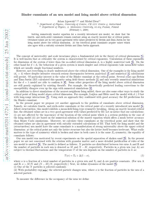
a r X i v :c o n d -m a t /0201472v 1 [c o n d -m a t .s t a t -m e c h ] 25 J a n 2002Binder cumulants of an urn model and Ising model above critical dimensionAdam Lipowski 1),2)and Michel Droz 1)1)Department of Physics,University of Gen`e ve,CH 1211Gen`e ve 4,Switzerland 2)Department of Physics,A.Mickiewicz University,61-614Poznan,Poland(February 1,2008)Solving numerically master equation for a recently introduced urn model,we show that the fourth-and sixth-order cumulants remain constant along an exactly located line of critical points.Obtained values are in very good agreement with values predicted by Br´e zin and Zinn-Justin for the Ising model above the critical dimension.At the tricritical point cumulants acquire values which also agree with a suitably extended Br´e zin and Zinn-Justin approach.The concept of universality and scale invariance plays a fundamental role in the theory of critical phenomena [1].It is well known that at criticality the system is characterized by critical exponents.Calculation of these exponents for dimension of the system d lower than the so-called critical dimension d c is a highly nontrivial task [2].On the other hand for d >d c the behaviour of a given system is much simpler and critical exponents take mean-ﬁeld values which are usually simple fractional numbers.However,not everything is clearly understood above the critical dimension.One of the examples is the Ising model (d c =4)where despite intensive research serious discrepancies between analytical [3]and numerical [4]calculations still persist.Of particular interest is the value of the Binder cumulant at the critical point.Several years ago Br´e zin and Zinn-Justin (BJ)calculated this quantity using ﬁeld theory methods [5]and only recently numerical simulations for the d =5model are able to conﬁrm it [6].Some other properties of the Ising model above critical dimension are still poorly explained by existing theories.For example,the theoretically predicted leading corrections to the susceptibility disagree even up the sign with numerical simulations [4].In addition to direct simulations of the nearest-neighbour Ising model,there are also some other ways to study the critical point of Ising model above critical dimension.For example,Luijten and Bl¨o te used the model with d ≤3but with long-range interactions [7].Using such an approach they conﬁrmed with good accuracy the BJ predictions for the Binder cumulant.In the present paper we propose yet another approach to the problem of cumulants above critical ly,we calculate fourth-and sixth-order cumulants at the critical point of a recently introduced urn model [8].Albeit structureless,this model exhibits a mean-ﬁeld Ising-type symmetry breaking.Along an exactly located critical line,the obtained values are in a very good agreement with values predicted by BJ.Let us notice that our calculations:(i)are not aﬀected by the inaccuracy of the location of the critical point which is a serious problem in the case of the Ising model (ii)are based on the numerical solution of the master equation which oﬀers a much better accuracy than Monte Carlo simulations.Moreover,we calculate these cumulants at the tricritical point and show that the obtained values are also in agreement with suitably extended calculations of BJ.That both the Ising model and the (structureless)urn model have the same cumulants is a manifestation of strong universality above the upper critical dimension:at the critical point not only the lattice structure but also the lattice itself becomes irrelevant.What really matters is the type of symmetry which is broken and since in both cases it is the same Z 2symmetry,the equality of cumulants follows.Our urn model was motivated by recent experiments on the spatial separation of shaken sand [9].In the present paper we are not concerned with the relation with granular matter and a more detailed justiﬁcation of rules of the urn model is omitted [8].The model is deﬁned as follows:N particles are distributed between two urns A and B and the number of particles in each urn is denoted as M and N −M ,respectively.Particles in a given urn (say A)are subject to thermal ﬂuctuations and the temperature T of the urn depends on the number of particles in it as:T (x )=T 0+∆(1−x ),(1)where x is a fraction of a total number of particles in a given urn and T 0and ∆are positive constants.(For urn A and B,x =M/N and (N −M )/N ,respectively.)Next,we deﬁne dynamics of the model [8]:(i)One of the N particles is selected randomly.(ii)With probability exp[−1ǫ=2M−NN−1T(<M/N>)]=<N−M>exp[−12+<ǫ>)exp[−12+<ǫ>)]=(1T(1∆/2−∆/2,0<∆<23,T0=√3.Let us notice that a random selection ofparticles implies basically the mean-ﬁeld nature of this model.Consequently,at the critical pointβ=1/2andγ≈1 (measured from the divergence of the variance of the order parameter),which are ordinary mean-ﬁeld exponents. However,the calculation of the dynamical exponent z gives z=0.50(1)[8]while the mean-ﬁeld value is2.We do not have convincing arguments which would explain such a small value of z.Presumably,this fact might be related with a structureless nature of our model.Deﬁning p(M,t)as the probability that in a given urn(say A)at the time t there are M particles,the evolution of the model is described by the following master equationp(M,t+1)=N−M+1Np(M+1,t)ω(M+1)+ p(M,t){MN[1−ω(N−M)]}for M=1,2...N−1p(0,t+1)=1Np(N−1,t)ω(1)+p(N,t)[1−ω(N)],(6) whereω(M)=exp[−1<ǫ2>2,x6=<ǫ6> N−18,12and2x 4=14)]4≈2.188440...,x 6=34)]4≈6.565319....(9)The fact that one can restrict the expansion of the free energy to the lowest order term is by no means obvious [3].Such a restriction leads to the correct results but only above critical dimension where the model behaves according to the mean-ﬁeld scenario with ﬂuctuations playing negligible role.For d <d c additional terms in the expansion are also important and cumulants take diﬀerent value.Numerical conﬁrmation of the above results requires extensive Monte Carlo simulations,and a satisfactory conﬁrmation was obtained only for x 4[6,10].Omitting detailed ﬁeld theory analysis,we can extend the BJ approach to the tricritical point.At such a point also the quartic term vanishes which makes the sixth-order term the leading one and the probability distribution gets theform p (x )∼e −x 6.Simple calculations for such a distribution yieldx 4=Γ(56)2)2=2,x 6=Γ(16Γ(13(tricritical point).Arrows indicate the BJ results for the critical and the tricritical point.3456700.0020.0040.0060.0080.01x 6(N )1/NFIG.2.The same as in Fig.1but for the sixth-order cumulant x 6(N ).The BJ results (9)-(10)are indicated by small arrows in Figs.1-2.Even without any extrapolation one can see,especially for critical points,a good agreement with our results.Data in Figs.1-2shows strong ﬁnite-size corrections.To have a better estimations of asymptotic values in the limit N →∞we assume ﬁnite size corrections of the formx 4,6(N )=x 4,6(∞)+AN −ω.(11)The least-square ﬁtting of our ﬁnite-N data to eq.(11)gives x 4,6(∞)which agree with BJ values (9)-(10)within the accuracy better than 0.1%.A better estimation of the correction exponent ωis obtained assuming that x 4,6(∞)are given by the BJ values.The exponent ωequals then the slope of the date in the logarithmic scale as presented in Figs.3-4.Our data shows that for the critical(tricritical)point ω=13).Let us notice that leading ﬁnite-size corrections to the Binder cumulant in the d =5Ising model at the critical point are also of the form N −0.5(with N being the linear system size)[7].Moreover,for the tricritical point but d <d c the probability distribution is known to exhibit a three-peak structure [11],which is diﬀerent than the single-peak formp (x )∼e −x 6.-2-1.5-1-0.500.512 2.533.544.55l o g 10[x 4,6(B J )-x 4,6(N )]log 10(N)FIG.3.Logarithmic plot of x 4(BJ )−x 4(N )(+)and x 6(BJ )−x 6(N )(×)as a function for N for ∆=0.5.Dotted straight lines have slope 0.5.-1.4-1.2-1-0.8-0.6-0.4-0.200.20.422.533.544.55l o g 10[x 4,6(B J )-x 4,6(N )]log 10(N)FIG.4.Logarithmic plot of x 4(BJ )−x 4(N )(+)and x 6(BJ )−x 6(N )(×)as a function fo N for ∆=23.In summary,we calculated fourth-and sixth-order cumulants at the critical and tricritical points in an urn modelwhich undergoes a symmetry breaking transition.Our results conﬁrm that,as predicted by Br´e zin and Zinn-Justin,the critical probability distributions of the rescaled order parameter has the form p (x )∼e −x 4.Similarly,for thetricritical point our results suggest that p (x )∼e −x 6.Although in our opinion convincing,the results are obtained using numerical methods.It would be desirable to have analytical arguments for the generation of such probability distributions.It seems that for the presented urn model this might be easier than for the Ising-type models.Let us notice that for the simplest urn model,which was introduced by Ehrenfest [12],the steady-state probability distribution can be calculated exactly in the continuumlimit of the master equation and the result has the form p (x )∼e −x 2,where x is now proportional to the diﬀerenceof occupancy ǫ.In the Ehrenfest model there is no critical point and we expect that a distribution of the type e −x2might characterize our model but oﬀthe critical line(in the symmetric phase).We hope that when suitably extended, an analytic approach to our model might extract critical and tricritical distributions as well.Such an approach is left as a future problem.ACKNOWLEDGMENTSThis work was partially supported by the Swiss National Science Foundation and the project OFES00-0578”COSYC OF SENS”.。

材料导论中英文讲稿 (58)

Module 7-video 12What are particle-reinforced composites？什么是颗粒增强复合材料？Hello！Welcome to Introduction to Materials. Today, we are going to talk about particle-reinforced composites, also called particle or particulate composites.译文：大家好！欢迎走进《材料导论》课堂。

今天，我们来一起学习颗粒增强复合材料。

Particle composites containing reinforcing particles of one or more materials suspended in a matrix of a different materials. As with nearly all materials, structure determines properties, and so it is with particle composites.This Figure illustrates the geometrical and spatial characteristics of particles, such as the concentration, size, shape，distribution and orientation. They all contribute to the properties of these materials. 颗粒增强复合材料由基体和分散相构成，分散相粒子的几何和空间特性，如含量、大小、形状、分布、取向等结构因素都会影响颗粒复合材料的性能。

译文：颗粒增强复合材料是由一种或多种增强颗粒分散于另一种基体材料中构成的复合材料。

颗粒增强复合材料与其它几乎所有材料一样，其结构决定着性能。

From Little Bangs to the Big Bang

a r X i v :a s t r o -p h /0504501v 1 22 A p r 2005From Little Bangs to the Big BangJohn EllisTheory Division,Physics Department,CERN,CH-1211Geneva 23,Switzerland E-mail:john.ellis@cern.ch CERN-PH-TH/2005-070astro-ph/0504501Abstract.The ‘Little Bangs’made in particle collider experiments reproduce the conditions in the Big Bang when the age of the Universe was a fraction of a second.It is thought that matter was generated,the structures in the Universe were formed and cold dark matter froze out during this very early epoch when the equation of state of the Universe was dominated by the quark-gluon plasma (QGP).Future Little Bangs may reveal the mechanism of matter generation and the nature of cold dark matter.Knowledge of the QGP will be an essential ingredient in quantitative understanding of the very early Universe..1.The Universe is Expanding The expansion of the Universe was ﬁrst established by Hubble’s discovery that distant galaxies are receding from us,with redshifts proportional to their relative distances from us.Extrapolating the present expansion backwards,there is good evidence that the Universe was once 3000times smaller and hotter than today,provided by the cosmic microwave background (CMB)radiation.This has a thermal distribution and is very isotropic,and is thought to have been released when electrons combined with ions from the primordial electromagnetic plasma to form atoms.The observed small dipole anisotropy is due to the Earth’s motion relative to this cosmic microwave background,and the very small anisotropies found by the COBE satellite are thought to have led to the formation of structures in the Universe,as discussed later [1].Extrapolating further back in time,there is good evidence that the Universe was once a billion times smaller and hotter than today,provided by the abundances of light elements cooked in the Big Bang [2].The Universe contains about 24%by mass of 4He,and somewhat less Deuterium,3He and 7Li.These could only have been cooked by nuclear reactions in the very early Universe,when it was a billion times smaller and hotter than today.The detailed light-element abundances depend on the amount of matter in the Universe,and comparison between observations and calculations suggests that there is not enough matter to stop the present expansion,or even to explain the amount of matter in the galaxies and their clusters.The calculations of the light-element abundances also depend on the number of particle types,and in particular on the number of diﬀerent neutrino types.This is now known from particle collider experiments to be three [3],with a corresponding number of charged leptons and quark pairs.2.The Very Early Universe and the Quark-Gluon PlasmaWhen the Universe was very young:t →0,also the scale factor a characterizing its size would have been very small:a →0,and the temperature T would have been very large,withcharacteristic relativistic particle energies E ∼T .In normal adiabatic expansion,T ∼1/a ,and,while the energy density of the Universe was dominated by relativistic matter,t ∼1/T 2.The following are some rough orders of magnitude:when the Universe had an age t ∼1second,the temperature was T ∼10,000,000,000degrees,and characteristic thermal energies were E ∼1MeV,comparable with the mass of theelectron.It is clear that one needs particle physics to describe the earlier history of the Universe [1].The very early Universe was presumably ﬁlled with primordial quark-gluon plasma (QGP).When the Universe was a few microseconds old,it is thought to have exited from this QGP phase,with the available quarks and gluons combining to make mesons and baryons.The primordial QGP would have had a very low baryon chemical potential µ.Experiments with RHIC reproduce cosmological conditions more closely than did previous SPS experiments,as seen in Fig.1,and the LHC will provide [4]an even closer approximation to the primordial QGP.I shall not discuss here the prospects for discovering quark matter inside dense astrophysical objects such as neutron stars,which would have a much larger baryon chemical potential.TµTc ~ 170 MeV µ ∼ o 922 MeV Figure 1.The phase diagram of hot and dense QCD for diﬀerent values of the baryon chemical potential µand temperature T [5],illustrating the physics reaches of SPS,RHIC and the ALICE experiment at the LHC [4].To what extent can information about the early Universe cast light on the quark-hadron phase transition?The latest lattice simulations of QCD with two light ﬂavours u,d and one moderately heavy ﬂavour s suggest that there was no strong ﬁrst-order transition.Instead,there was probably a cross-over between the quark and hadron phases,see,for example,Fig.2[5],during which the smooth expansion of the Universe is unlikely to have been modiﬁed substantially.Speciﬁcally,it is not thought that this transition would have induced inhomogeneities large enough to have detectable consequences today.3.Open Cosmological QuestionsThe Standard Model of cosmology leaves many important questions unanswered.Why is the Universe so big and old?Measurements by the WMAP satellite,in particular,indicate that its age is about 14,000,000,000years [6].Why is its geometry nearly Euclidean?Recent data indicate that it is almost ﬂat,close to the borderline for eternal expansion.Where did the matter come from?The cosmological nucleosynthesis scenario indicates that there is approximately one proton in the Universe today for every 1,000,000,000photons,and no detectable amount0.81 1.2 1.4 1.6 1.82T/T 000.20.40.60.8µq /T =0.8µq /T =1.0µq /T =0.6µq /T =0.4µq /T =0.2∆(p/T 4)Figure 2.The growth of the QCD pressure with temperature,for diﬀerent values of the baryon chemical potential µ[5].The rise is quite smooth,indication that there is not a strong ﬁrst-order phase transition,and probably no dramatic consequences in the early Universe.of antimatter.How did cosmological structures form?If they did indeed form from the ripples observed in the CMB,how did these originate?What is the nature of the invisible dark matter thought to ﬁll the Universe?Its presence is thought to have been essential for the ampliﬁcation of the primordial perturbations in the CMB.It is clear that one needs particle physics to answer these questions,and that their solutions would have operated in a Universe ﬁlled with QGP.4.A Strange Recipe for a UniverseAccording to the ‘Concordance Model’suggested by a multitude of astrophysical and cosmological observations,the total density of the Universe is very close to the critical value:ΩT ot =1.02±0.02,as illustrated in Fig.3[6].The theory of cosmological inﬂation suggests that the density should be indistinguishable from the critical value,and this is supported by measurements of the CMB.On the other hand,the baryon density is small,as inferred not only from Big-Bang nucleosynthesis but also and independently from the CMB:ΩBaryons ∼few%.The CMB information on these two quantities comes from observations of peaks in the ﬂuctuation spectrum in speciﬁc partial waves corresponding to certain angular scales:the position of the ﬁrst peak is sensitive to ΩT ot ,and the relative heights of subsequent peaks are sensitive to ΩBaryons .The fraction Ωm of the critical density provided by all forms of matter is not very well constrained by the CMB data alone,but is quite tightly constrained by combining them with observations of high-redshift supernovae [7]and/or large-scale structures [8],each of which favours ΩMatter ∼0.3,as also seen in Fig.3.As seen in Fig.4,there is good agreement between BBN calculations and astrophysical observations for the Deuterium and 4He abundances [2].The agreement for 7Li is less striking,though not disastrously bad 1.The good agreement between the corresponding 1It seems unlikely that the low abundance of 7Li observed could have been modiﬁed signiﬁcantly by the decaysFigure3.The density of matterΩm and dark energyΩΛinferred from WMAP and other CMB data(WMAPext),and from combining them with supernova and Hubble Space Telescope data[6].determinations ofΩBaryons obtained from CMB and Big-Bang nucleosynthesis calculations in conventional homogeneous cosmology imposes important constraints on inhomogeneous models of nucleosynthesis.In particular,they exclude the possibility thatΩBaryons might constitute a large fraction ofΩT ot.Signiﬁcant inhomogeneities might have been generated at the quark-hadron phase transition,if it was stronglyﬁrst-order[10].Although,as already discussed,lattice calculations suggest that this is rather unlikely,heavy-ion collision experiments must be theﬁnal arbiter on the nature of the quark-hadron phase transition.5.Generating the Matter in the UniverseAs was pointed out by Sakharov[11],there are three essential requirements for generating the matter in the Universe via microphysics.First,one needs a diﬀerence between matter and antimatter interactions,as has been observed in the laboratory in the forms of violations of C and CP in the weak interactions.Secondly,one needs interactions that violate the baryon and lepton numbers,which are present as non-perturbative electroweak interactions and in grand uniﬁed theories,but have not yet been seen.Finally,one needs a breakdown of thermal equilibrium, which is possible during a cosmological phase transition,for example at the GUT or electroweak scale,or in the decays of heavy particles,such as a heavy singlet neutrinoνR[12].The issueof heavy particles[9]:it would be valuable to reﬁne the astrophysical determinations.Figure4.Primordial light element abundances as predicted by BBN(light)and WMAP(dark shaded regions)[2],for(a)D/H,(b)the4He abundance Y p and(c)7Li/H[2].then is whether we will be able to calculate the resulting matter density in terms of laboratory measurements.Unfortunately,the Standard Model C and CP violation measured in the quark sector seem unsuitable for baryogenesis,and the electroweak phase transition in the Standard Model would have been second order.However,additional CP violation and aﬁrst-order phase transition in an extended electroweak Higgs sector might have been able to generate the matter density[13],and could be testable at the LHC and/or ILC.An alternative is CP violation in the lepton sector,which could be probed in neutrino oscillation experiments,albeit indirectly, or possibly in the charged-lepton sector,which might be related more directly to the matter density[14].In any case,detailed knowledge of the QGP equation of state would be necessary if one were ever to hope to be able to calculate the baryon-to-entropy ratio with an accuracy of a few percent.6.The Formation of Structures in the UniverseThe structures seen in the Universe-clusters,galaxies,stars and eventually ourselves-are all thought to have developed from primordialﬂuctuations in the CMB.This idea is supported visually by observations of galaxies,which look smooth at the largest scales at high redshifts, but cluster at smaller scales at low redshifts[15].This scenario requires ampliﬁcation of the smallﬂuctuations observed in the CMB,which is possible with massive non-relativistic weakly-interacting particles.On the other hand,relativistic light neutrinos would have escaped from smaller structures,and so are disfavoured as ampliﬁers.Non-relativistic‘cold dark matter’is preferred,as seen in a comparison of the available data on structures in the Universe with the cosmological Concordance Model[8].The hot news in the observational tests of this scenario has been the recent detection of baryonic ripples from the Big Bang[16],as seen in Fig.5.These are caused by sound waves spreading out from irregularities in the CMB,which show up in the correlation function between structures in the(near-)contemporary Universe as features with a characteristic size.In addition to supporting the scenario of structure formation by ampliﬁcation of CMBﬂuctuations, these observations provide measurements of the expansion history and equation of state of the Universe.Figure5.The baryonic‘ripple’in the large-scale correlation function of luminous red galaxies observed in the Sloan Digital Sky Survey of galactic redshifts[16].7.Do Neutrinos Matter?Oscillation experiments tell us that neutrinos have very small but non-zero masses[17,18], and so must make up at least some of the dark matter.As already mentioned,since such light neutrinos move relativistically during the epoch of structure formation,they would have escaped from galaxies and not contributed to their formation,whereas they could have contributed to the formation of clusters.Conversely,the success of the cosmological Concordance Model enables one to set a cosmological upper limit on the sum of light neutrino masses,as seen in Fig.6:Σνmν<0.7eV[6],which is considerably more sensitive than direct laboratory searches.In the future,this cosmological sensitivity might attain the range indicated by atmospheric neutrino data[17].However,even if no dark matter eﬀect of non-zero light neutrino masses is observed,this does not mean that neutrinos have no cosmological role,since unstable heavier neutrinos might have generated matter via the Sakharov mechanism[11].8.Particle Dark Matter CandidatesCandidates for the non-relativistic cold dark matter required to amplify CMBﬂuctuations include the axion[19],TeV-scale weakly-interacting massive particles(WIMPs)produced thermally in the early Universe,such as the lightest supersymmetric partner of a Standard Model particle(probably the lightest neutralinoχ),the gravitino(which is likely mainly to have been produced in the very early Universe,possibly thermally),and superheavy relic particles that might have been produced non-thermally in the very early Universe[20](such as the‘cryptons’predicted in some string models[21]).9.Supersymmetric Dark MatterSupersymmetry is a very powerful symmetry relating fermionic‘matter’particles to bosonic ‘force’particles[22].Historically,the original motivations for supersymmetry were purely theoretical:its intrinsic beauty,its ability to tame inﬁnities in perturbation theory,etc.The ﬁrst phenomenological motivation for supersymmetry at some accessible energy was that itFigure6.The likelihood function for the total neutrino densityΩνh2derived by WMAP[6]. The upper limit mν<0.23eV applies if there are three degenerate neutrinos.might also help explain the electroweak mass scale,by stabilizing the hierarchy of mass scales in physics[23].It was later realized also that the lightest supersymmetric particle(LSP)would be stable in many models[24].Moreover,it should weigh below about1000GeV,in order to stabilize the mass hierarchy,in which case its relic density would be similar to that required for cold dark matter[25].As described below,considerable eﬀort is now put into direct laboratory searches for supersymmetry,as well as both direct and indirect astrophysical searches.Here I concentrate on the minimal supersymmetric extension of the Standard Model(MSSM), in which the Standard Model particles acquire superpartners and there are two doublets of Higgs ﬁelds.The interactions in the MSSM are completely determined by supersymmetry,but one must postulate a number of soft supersymmetry-breaking parameters,in order to accommodate the mass diﬀerences between conventional particles and their superpartners.These parameters include scalar masses m0,gaugino masses m1/2,and trilinear soft couplings A0.It is often assumed that these parameters are universal,so that there is a single m0,a single m1/2,and a single A0parameter at the input GUT scale,a scenario called the constrained MSSM(CMSSM). However,there is no deep theoretical justiﬁcation for this universality assumption,except in minimal supergravity models.These models also make a prediction for the gravitino mass: m3/2=m0,which is not necessarily the case in the general CMSSM.As already mentioned,the lightest supersymmetric particle is stable in many models,this because of the multiplicative conservation of R parity,which is a combination of spin S,lepton number L and baryon number B:R=(−1)2S−L+3B.It is easy to check that conventional particles have R=+1and sparticles have R=−1.As a result,sparticles are always produced in pairs,heavier sparticles decay into lighter ones,and the lightest supersymmetric particle (LSP)is stable.The LSP cannot have strong or electromagnetic interactions,because these would bind it toconventional matter,creating bound states that would be detectable as anomalous heavy nuclei.Among the possible weakly-interacting scandidates for the LSP,one ﬁnds the sneutrino ,which has been excluded by a combination of LEP and direct searches for astrophysical dark matter,the lightest neutralino χ,and the gravitino .There are good prospects for detecting the neutralino or gravitino in collider experiments,and neutralino dark matter may also be detectable either directly or indirectly,but gravitino dark matter would be a nightmare for detection.10.Constraints on SupersymmetryImportant constraints on supersymmetry are imposed by the absences of sparticles at LEP and the Tevatron collider,implying that sleptons and charginos should weigh >100GeV [26],and that squarks and gluinos should weigh >250GeV,respectively.Important indirect constraints are imposed by the LEP lower limit on the mass of the lightest Higgs boson,114GeV [27],and the experimental measurement of b →sγdecay [28],which agrees with the Standard Model.The measurement of the anomalous magnetic moment of the muon,g µ−2,also has the potential to constrain supersymmetry,but the signiﬁcance of this constraint is uncertain,in the absence of agreement between the e +e −annihilation and τdecay data used to estimate the Standard Model contribution to g µ−2[29].Finally,one of the strongest constraints on the supersymmetric parameter space is that imposed by the density of dark matter inferred from astrophysical and cosmological observations.If this is composed of the lightest neutralino χ,one has 0.094<Ωχh 2<0.129[6],and it cannot in any case be higher than this.For generic domains of the supersymmetric parameter space,this range constrains m 0with an accuracy of a few per cent as a function of m 1/2,as seen in Fig.7[30].m 0 (G e V )m 1/2 (GeV)m 0 (G e V )m 1/2 (GeV)Figure 7.The (m 1/2,m 0)planes for (a)tan β=10and tan β=50with µ>0and A 0=0,assumingm t =175GeV and m b (m b )Figure8.The factor h eﬀ(T)calculated using diﬀerent equations of state[31].11.The Relic Density and the Quark-Gluon PlasmaThe accurate calculation of the relic density depends not only on the supersymmetric model parameters,but also on the eﬀective Hubble expansion rate as the relic particles annihilate and freeze out of thermal equilibrium[25]:˙n+3Hn=−<σann v>(n2−n2eq).This is,in turn,sensitive to the eﬀective number of particle species:Y0≃ 4521g eff 13d ln h effm N L V S P (G e V )m LVSP (GeV)Figure 9.Scatter plot of the masses of the lightest visible supersymmetric particle (LVSP)and the next-to-lightest visible supersymmetric particle (NLVSP)in the CMSSM.The darker (blue)triangles satisfy all the laboratory,astrophysical and cosmological constraints.For comparison,the dark (red)squares and medium-shaded (green)crosses respect the laboratory constraints,but not those imposed by astrophysics and cosmology.In addition,the (green)crosses represent models which are expected to be visible at the LHC.The very light (yellow)points are those for which direct detection of supersymmetric dark matter might be possible [33].13.Strategies for Detecting Supersymmetric Dark MatterThese include searches for the annihilations of relic particles in the galactic halo:χχ→antiprotons or positrons,annihilations in the galactic centre:χχ→γ+...,annihilations in the core of the Sun or the Earth:χχ→ν+···→µ+···,and scattering on nuclei in the laboratory:χA →chiA .After some initial excitement,recent observations of cosmic-ray antiprotons are consistent with production by primary matter cosmic rays.Moreover,the spectra of annihilation positrons calculated in a number of CMSSM benchmark models [32]seem to fall considerably below the cosmic-ray background [37].Some of the spectra of photons from annihilations in Galactic Centre,as calculated in the same set of CMSSM benchmark scenarios,may rise above the expected cosmic-ray background,albeit with considerable uncertainties due to the unknown enhancement of the cold dark matter density.In particular,the GLAST experiment may have the best chance of detecting energetic annihilation photons [37],as seen in the left panel of Fig.10.Annihilations in the Solar System also oﬀer detection prospects in some of the benchmark scenarios,particularly annihilations inside the Sun,which might be detectable in experiments such as AMANDA,NESTOR,ANTARES and particularly IceCUBE,as seen in the right panel of Fig.10[37].The rates for elastic dark matter scattering cross sections calculated in the CMSSM are typically considerably below the present upper limit imposed by the CDMS II experiment,in both the benchmark scenarios and the global ﬁt to CMSSM parameters based on present data [38].However,if the next generation of direct searches for elastic scattering can reach a sensitivity of 10−10pb,they should be able to detect supersymmetric dark matter in many supersymmetric scenarios.Fig.11compares the cross sections calculated under a relatively optimistic assumption for the relevant hadronic matrix element σπN =64MeV,for choices of CMSSM parameters favoured at the 68%(90%)conﬁdence level in a recent analysis using theFigure 10.Left panel:Spectra of photons from the annihilations of dark matter particles in the core of our galaxy,in diﬀerent benchmark supersymmetric models [37].Right panel:Signals for muons produced by energetic neutrinos originating from annihilations of dark matter particles in the core of the Sun,in the same benchmark supersymmetric models [37].10-1210-1110-1010-910-810-710-610-50 200 400 600800 1000σ (p b )m χ (GeV)CMSSM, tan β=10, µ>0Σ=64 MeV CDMS II CL=90%CL=68%10-1210-1110-1010-910-810-710-610-5 0 200 400 600 800 1000σ (p b )m χ (GeV)CMSSM, tan β=50, µ>0Σ=64 MeV CDMS II CL=90%CL=68%Figure 11.Scatter plots of the spin-independent elastic-scattering cross section predicted in the CMSSM for (a)tan β=10,µ>0and (b)tan β=50,µ>0,each with σπN =64MeV [38].The predictions for models allowed at the 68%(90%)conﬁdence levels [39]are shown by blue ×signs (green +signs).observables m W ,sin 2θW ,b →sγand g µ−2[39].14.Connections between the Big Bang and Little BangsAstrophysical and cosmological observations during the past few years have established a Concordance Model of cosmology,whose matter content is quite accurately determined.Most of the present energy density of the Universe is in the form of dark vacuum energy,with about 25%in the form of dark matter,and only a few %in the form of conventional baryonic matter.Two of the most basic questions raised by this Concordance Model are the nature of the dark matter and the origin of matter.Only experiments at particle colliders are likely to be able to answer these and other fundamental questions about the early Universe.In particular,experiments at the LHC will recreate quark-gluon plasma conditions similar to those when the Universe was less than a microsecond old[4],and will oﬀer the best prospects for discovering whether the dark matter is composed of supersymmetric particles[40,41].LHC experiments will also cast new light on the cosmological matter-antimattter asymmetry[42].Moreover,discovery of the Higgs boson will take us closer to the possibilities for inﬂation and dark energy.There are many connections between the Big Bang and the little bangs we create with particle colliders.These connections enable us both to learn particle physics from the Universe,and to use particle physics to understand the Universe.References[1]J.R.Ellis,Lectures given at16th Canberra International Physics Summer School on The New Cosmology,Canberra,Australia,3-14Feb2003,arXiv:astro-ph/0305038;K.A.Olive,TASI lectures on Astroparticle Physics,arXiv:astro-ph/0503065.[2]R.H.Cyburt, B. D.Fields,K. A.Olive and E.Skillman,Astropart.Phys.23(2005)313[arXiv:astro-ph/0408033].[3]LEP Electroweak Working Group,http://lepewwg.web.cern.ch/LEPEWWG/Welcome.html.[4]ALICE Collaboration,http://pcaliweb02.cern.ch/NewAlicePortal/en/Collaboration/index.html.[5] C.R.Allton,S.Ejiri,S.J.Hands,O.Kaczmarek,F.Karsch,ermann and C.Schmidt,Nucl.Phys.Proc.Suppl.141(2005)186[arXiv:hep-lat/0504011].[6] D.N.Spergel et al.[WMAP Collaboration],Astrophys.J.Suppl.148(2003)175[arXiv:astro-ph/0302209].[7] A.G.Riess et al.[Supernova Search Team Collaboration],Astron.J.116(1998)1009[arXiv:astro-ph/9805201];S.Perlmutter et al.[Supernova Cosmology Project Collaboration],Astrophys.J.517(1999)565[arXiv:astro-ph/9812133].[8]N. A.Bahcall,J.P.Ostriker,S.Perlmutter and P.J.Steinhardt,Science284(1999)1481[arXiv:astro-ph/9906463].[9]J.R.Ellis,K.A.Olive and E.Vangioni,arXiv:astro-ph/0503023.[10]K.Jedamzik and J.B.Rehm,Phys.Rev.D64(2001)023510[arXiv:astro-ph/0101292].[11] A.D.Sakharov,Pisma Zh.Eksp.Teor.Fiz.5(1967)32[JETP Lett.5(1967SOPUA,34,392-393.1991UFNAA,161,61-64.1991)24].[12]M.Fukugita and T.Yanagida,Phys.Lett.B174(1986)45.[13]See,for example:M.Carena,M.Quiros,M.Seco and C.E.M.Wagner,Nucl.Phys.B650(2003)24[arXiv:hep-ph/0208043].[14]See,for example:J.R.Ellis and M.Raidal,Nucl.Phys.B643(2002)229[arXiv:hep-ph/0206174].[15]The2dF Galaxy Redshift Survey,.au/2dFGRS/.[16] D.J.Eisenstein et al.,arXiv:astro-ph/0501171;S.Cole et al.[The2dFGRS Collaboration],arXiv:astro-ph/0501174.[17]Y.Fukuda et al.[Super-Kamiokande Collaboration],Phys.Rev.Lett.81(1998)1562[arXiv:hep-ex/9807003].[18]See,for example:Q.R.Ahmad et al.[SNO Collaboration],Phys.Rev.Lett.87(2001)071301[arXiv:nucl-ex/0106015].[19]See,for example:S.Andriamonje et al.[CAST Collaboration],Phys.Rev.Lett.94(2005)121301[arXiv:hep-ex/0411033].[20] D.J.H.Chung,E.W.Kolb and A.Riotto,Phys.Rev.D59(1999)023501[arXiv:hep-ph/9802238].[21]K.Benakli,J.R.Ellis and D.V.Nanopoulos,Phys.Rev.D59(1999)047301[arXiv:hep-ph/9803333].[22]J.Wess and B.Zumino,Nucl.Phys.B70(1974)39.[23]L.Maiani,Proceedings of the1979Gif-sur-Yvette Summer School On Particle Physics,1;G.’t Hooft,inRecent Developments in Gauge Theories,Proceedings of the Nato Advanced Study Institute,Cargese,1979, eds.G.’t Hooft et al.,(Plenum Press,NY,1980);E.Witten,Phys.Lett.B105(1981)267.[24]P.Fayet,Uniﬁcation of the Fundamental Particle Interactions,eds.S.Ferrara,J.Ellis andP.van Nieuwenhuizen(Plenum,New York,1980),p.587.[25]J.Ellis,J.S.Hagelin,D.V.Nanopoulos,K.A.Olive and M.Srednicki,Nucl.Phys.B238(1984)453;see alsoH.Goldberg,Phys.Rev.Lett.50(1983)1419.[26]The Joint LEP2Supersymmetry Working Group,http://lepsusy.web.cern.ch/lepsusy/.[27]LEP Higgs Working Group for Higgs boson searches,OPAL Collaboration,ALEPH Collaboration,DELPHICollaboration and L3Collaboration,Phys.Lett.B565(2003)61[arXiv:hep-ex/0306033].Search for neutral Higgs bosons at LEP,paper submitted to ICHEP04,Beijing,LHWG-NOTE-2004-01,ALEPH-2004-008,DELPHI-2004-042,L3-NOTE-2820,OPAL-TN-744,http://lephiggs.web.cern.ch/LEPHIGGS/papers/August2004。

材料科学与工程专业英语Unit2ClassificationofMaterials译文

Unit 2 Classification of MaterialsSolid materials have been conveniently grouped into three basic classifications: metals, ceramics, and polymers. This scheme is based primarily on chemical makeup and atomic structure, and most materials fall into one distinct grouping or another, although there are some intermediates. In addition, there are three other groups of important engineering materials —composites, semiconductors, and biomaterials.译文：译文：固体材料被便利的分为三个基本的类型：金属，陶瓷和聚合物。

固体材料被便利的分为三个基本的类型：金属，陶瓷和聚合物。

这个分类是首先基于这个分类是首先基于化学组成和原子结构来分的，化学组成和原子结构来分的，大多数材料落在明显的一个类别里面，大多数材料落在明显的一个类别里面，大多数材料落在明显的一个类别里面，尽管有许多中间品。

尽管有许多中间品。

除此之外，此之外，有三类其他重要的工程材料－复合材料，半导体材料和生物材料。

有三类其他重要的工程材料－复合材料，半导体材料和生物材料。

Composites consist of combinations of two or more different materials, whereas semiconductors are utilized because of their unusual electrical characteristics; biomaterials are implanted into the human body. A brief explanation of the material types and representative characteristics is offered next.译文：复合材料由两种或者两种以上不同的材料组成，然而半导体由于它们非同寻常的电学性质而得到使用；生物材料被移植进入人类的身体中。

Signature of a Pairing Transition in the Heat Capacity of Finite Nuclei

a rXiv:n ucl-t h /96v15Sep2Signature of a Pairing Transition in the Heat Capacity of Finite Nuclei S.Liu and Y.Alhassid Center for Theoretical Physics,Sloane Physics Laboratory,Yale University,New Haven,Connecticut 06520,U.S.A.(February 8,2008)Abstract The heat capacity of iron isotopes is calculated within the interacting shell model using the complete (pf +0g 9/2)-shell.We identify a signature of the pairing transition in the heat capacity that is correlated with the suppression of the number of spin-zero neutron pairs as the temperature increases.Our results are obtained by a novel method that signiﬁcantly reduces the statis-tical errors in the heat capacity calculated by the shell model Monte Carlo approach.The Monte Carlo results are compared with ﬁnite-temperature Fermi gas and BCS calculations.Typeset using REVT E XPairing eﬀects inﬁnite nuclei are well known;examples include the energy gap in the spectra of even-even nuclei and an odd-even eﬀect observed in nuclear masses.However,less is known about the thermal signatures of the pairing interaction in nuclei.In a macroscopic conductor,pairing leads to a phase transition from a normal metal to a superconductor below a certain critical temperature,and in the BCS theory[1]the heat capacity is characterized by aﬁnite discontinuity at the transition temperature.As the linear dimension of the system decreases below the pair coherence length,ﬂuctuations in the order parameter become important and lead to a smooth transition.The eﬀects of both staticﬂuctuations[2,3] and small quantalﬂuctuations[4]have been explored in studies of small metallic grains.A pronounced peak in the heat capacity is observed for a large number of electrons,but for less than∼100electrons the peak in the heat capacity all but disappears.In the nucleus,the pair coherence length is always much larger than the nuclear radius,and large ﬂuctuations are expected to suppress any singularity in the heat capacity.An interesting question is whether any signature of the pairing transition still exists in the heat capacity of the nucleus despite the largeﬂuctuations.When only static and small-amplitude quantal ﬂuctuations are taken into account,a shallow‘kink’could still be seen in the heat capacity of an even-even nucleus[5].This calculation,however,was limited to a schematic pairing model.Canonical heat capacities were recently extracted from level density measurements in rare-earth nuclei[6]and were found to have an S-shape that is interpreted to represent the suppression of pairing correlations with increasing temperature.The calculation of the heat capacity of theﬁnite interacting nuclear system beyond the mean-ﬁeld and static-path approximations is a diﬃcult problem.Correlation eﬀects due to residual interactions can be accounted for in the framework of the interacting nuclear shell model.However,atﬁnite temperature a large number of excited states contribute to the heat capacity and very large model spaces are necessary to obtain reliable results.The shell model Monte Carlo(SMMC)method[7,8]enables zero-andﬁnite-temperature calculations in large spaces.In particular,the thermal energy E(T)can be computed versus temperature T and the heat capacity can be obtained by taking a numerical derivative C=dE/dT.However,theﬁnite statistical errors in E(T)lead to large statistical errors in the heat capacity at low temperatures(even for good-sign interactions).Such large errors occur already around the pairing transition temperature and thus no deﬁnite signatures of the pairing transition could be identiﬁed.Furthermore,the large errors often lead to spurious structure in the calculated heat capacity.Presumably,a more accurate heat capacity can be obtained by a direct calculation of the variance of the Hamiltonian,but in SMMC such a calculation is impractical since it involves a four-body operator.The variance of the Hamiltonian has been calculated using a diﬀerent Monte Carlo algorithm[9],but that method is presently limited to a schematic pairing interaction.Here we report a novel method for calculating the heat capacity within SMMC that takes into account correlated errors and leads to much smaller statistical ing this method we are able to identify a signature of the pairing transition in realistic calculations of the heat capacity ofﬁnite nuclei.The signature is well correlated with the suppression in the number of spin-zero pairs across the transition temperature.The Monte Carlo approach is based on the Hubbard-Stratonovich(HS)representation of the many-body imaginary-time propagator,e−βH= D[σ]GσUσ,whereβis the in-verse temperature,Gσis a Gaussian weight and Uσis a one-body propagator that de-scribes non-interacting nucleons moving inﬂuctuating time-dependent auxiliaryﬁeldsσ. The canonical thermal expectation value of an observable O can be written as O = D[σ]GσTr(OUσ)/ D[σ]GσTr Uσ,where Tr denotes a canonical trace for N neutrons and Z protons.We can rewriteO = [Tr(OUσ)/Tr Uσ]ΦσWsamples.In particular the thermal energy can be calculated as a thermal average of the Hamilto-nian H .The heat capacity C =−β2∂E/∂βis then calculated by estimating the derivative as a ﬁnite diﬀerenceC =−β2E (β+δβ)−E (β−δβ)D [σ±]G σ±(β±δβ)Tr U σ±(β±δβ),(3)where the corresponding σﬁelds are denoted by σ±.To have the same number of time slices N t in the discretized version of (3)as in the original HS representation of E (β),we deﬁne modiﬁed time slices ∆β±by N t ∆β±=β±δβ.We next change integration variables in (3)from σ±to σaccording to σ±=(∆β/∆β±)1/2σ,so that the Gaussian weight is left unchanged G σ±(β±δβ)≡exp −αn12|v α|(σα(τn ))2∆β =G σ(β)(v αare the interaction ‘eigenvalues’,obtained by writing the interaction in a quadratic form αv αˆρ2α/2,where ˆραare one-body densities).Rewriting (3)using the measure D [σ](the Jacobian resulting from the change in integration variables is constant and canceled between the numerator and denominator),we ﬁndE (β±δβ)= Tr HU σ±(β±δβ)Tr U σ(β)Φσ W Tr U σ(β)Φσ W ≡H ±among the quantities H±and Z±,which would lead to a smaller error for C.The covariances among H±and Z±as well as their variances can be calculated in the Monte Carlo and used to estimate the correlated error of the heat capacity.We have calculated the heat capacity for the iron isotopes52−62Fe using the complete (pf+0g9/2)-shell and the good-sign interaction of Ref.[10].Fig.1demonstrates the sig-niﬁcant improvement in the statistical Monte Carlo errors.On the left panel of thisﬁgure we show the heat capacity of54Fe calculated in the conventional method,while the right panel shows the results from the new method.The statistical errors for T∼0.5−1MeV are reduced by almost an order of magnitude.The results obtained in the conventional calculation seem to indicate a shallow peak in the heat capacity around T∼1.25MeV,but the calculation using the improved method shows no such structure.The heat capacities of four iron isotopes55−58Fe,calculated with the new method,are shown in the top panel of Fig. 2.The heat capacities of the two even-mass iron isotopes (56Fe and58Fe)show a diﬀerent behavior around T∼0.7−0.8MeV as compared with the two odd-mass isotopes(55Fe and57Fe).While the heat capacity of the odd-mass isotopes increases smoothly as a function of temperature,the heat capacity of the even-mass isotopes is enhanced for T∼0.6−1MeV,increasing sharply and then leveling oﬀ,displaying a ‘shoulder.’This‘shoulder’is more pronounced for the isotope with more neutrons(58Fe). To correlate this behavior of the heat capacity with a pairing transition,we calculated the number of J=0nucleon pairs in these nuclei.A J=0pair operator is deﬁned as usual by∆†= a,m a>0(−1)j a−m aj a+1/2a†ja m aa†ja−m a,(5)where j a is the spin and m a is the spin projection of a single-particle orbit a.Pair-creation operators of the form(5)can be deﬁned for protons(∆†pp),neutrons(∆†nn),and proton-neutrons(∆†pn).The average number ∆†∆ of J=0pairs(of each type)can be calculated exactly in SMMC as a function of temperature.The bottom panel of Fig.2shows the number of neutron pairs ∆†nn∆nn for55−58Fe.At low temperature the number of neutron pairs for isotopes with an even number of neutrons is signiﬁcantly larger than that forisotopes with an odd number of neutrons.Furthermore,for the even-mass isotopes we observe a rapid suppression of the number of neutron pairs that correlates with the‘shoulder’observed in the heat capacity.The diﬀerent qualitative behavior in the number of neutron pairs versus temperature between odd-and even-mass iron isotopes provides a clue to the diﬀerence in their heat capacities.A transition from a pair-correlated ground state to a normal state at higher temperatures requires additional energy for breaking of neutron pairs, hence the steeper increase observed in the heat capacity of the even-mass iron isotopes. Once the pairs are broken,less energy is required to increase the temperature,and the heat capacity shows only a moderate increase.It is instructive to compare the SMMC heat capacity with a Fermi gas and BCS calcula-tions.The heat capacity can be calculated from the entropy using the relation C=T∂S/∂T. The entropy S of uncorrelated fermions is given byS(T)=− a[f a ln f a+(1−f a)ln(1−f a)],(6) with f a being theﬁnite-temperature occupation numbers of the single-particle orbits a.Above the pairing transition-temperature T c,f a are just the Fermi-Dirac occupancies f a= [1+eβ(ǫa−µ)]−1,whereµis the chemical potential determined from the total number of particles andǫa are the single-particle energies.Below T c,it is necessary to take into account the BCS solution which has lower free energy.Since condensed pairs do not contribute to the entropy,the latter is still given by(6)but f a are now the quasi-particle occupancies[1],1f a=(ǫa−µ)2+∆2are the quasi-particle energies,where the gap∆(T)and the chemical potentialµ(T)are determined from theﬁnite-temperature BCS equations.In practice,we treat protons and neutrons separately.We applied the Fermi gas and BCS approximations to estimate the heat capacities of the iron isotopes.To take into account eﬀects of a quadrupole-quadrupole interaction,we used an axially deformed Woods-Saxon potential to extract the single-particle spectrumǫa[11].A deformation parameterδfor the even iron isotopes can be extracted from experimental B(E2)values.However,since B(E2)values are not available for all of these isotopes,we used an alternate procedure.The excitation energy E x(2+1)of theﬁrst excited2+state in even-even nuclei can be extracted in SMMC by calculating J2 βat low temperatures and using a two-state model(the0+ground state and theﬁrst excited2+state)where J2 β≈6/(1+eβE x(2+1)/5)[12].The excitation energy of the2+1state is then used in the empirical formula of Bohr and Mottelson[13]τγ=(5.94±2.43)×1014E−4x(2+1)Z−2A1/3to estimate the meanγ-ray lifetimeτγand the corresponding B(E2).The deformation pa-rameterδis then estimated from B(E2)=[(3/4π)Zer20A2/3δ]2/5.Weﬁnd(using r0=1.27 fm)δ=0.225,0.215,0.244,0.222,0.230,and0.220for the even iron isotopes52Fe–62Fe, respectively.For the odd-mass iron isotopes we adapt the deformations in Ref.[14].The zero-temperature pairing gap∆is extracted from experimental odd-even mass diﬀerences and used to determine the pairing strength G(needed for theﬁnite temperature BCS solu-tion).The top panels of Fig.3show the Fermi-gas heat capacity(dotted-dashed lines)for 59Fe(right)and60Fe(left)in comparison with the SMMC results(symbols).The SMMC heat capacity in the even-mass60Fe is below the Fermi-gas estimate for T<∼0.5MeV, but is enhanced above the Fermi gas heat capacity in the region0.5<∼T<∼0.9MeV. The line shape of the heat capacity is similar to the S-shape found experimentally in the heat capacity of rare-earth nuclei[6].We remark that the saturation of the SMMC heat capacity above∼1.5MeV(and eventually its decrease with T)is an artifact of theﬁnite model space.The solid line shown for60Fe is the result of the BCS calculation.There are two‘peaks’in the heat capacity corresponding to separate pairing transitions for neutrons (T n c≈0.9MeV)and protons(T p c≈1.2MeV).Theﬁnite discontinuities in the BCS heat capacity are shown by the dotted lines.The pairing solution describes well the SMMC results for T<∼0.6MeV.However,the BCS peak in the heat capacity is strongly suppressed around the transition temperature.This is expected in theﬁnite nuclear system because of the strongﬂuctuations in the vicinity of the pairing transition(not accounted for in themean-ﬁeld approach).Despite the largeﬂuctuations,a‘shoulder’still remains around the neutron-pairing transition temperature.The bottom panels of Fig.3show the number of spin-zero pairs versus temperature in SMMC.The number of p-p and n-p pairs are similar in the even and odd-mass iron isotopes. However,the number of n-n pairs at low T diﬀers signiﬁcantly between the two isotopes. The n-n pair number of60Fe decreases rapidly as a function of T,while that of59Fe decreases slowly.The S-shape or shoulder seen in the SMMC heat capacity of60Fe correlates well with the suppression of neutron pairs.Fig.4shows the complete systematics of the heat capacity for the iron isotopes in the mass range A=52−62for both even-mass(left panel)and odd-mass(right panel). At low temperatures the heat capacity approaches zero,as expected.When T is high,the heat capacity for all isotopes converges to approximately the same value.In the intermediate temperature region(T∼0.7MeV),the heat capacity increases with mass due to the increase of the density of states with mass.Pairing leads to an odd-even staggering eﬀect in the mass dependence(see also in Fig.2)where the heat capacity of an odd-mass nucleus is signiﬁcantly lower than that of the adjacent even-mass nuclei.For example,the heat capacity of57Fe is below that of both56Fe and58Fe.The heat capacities of the even-mass58Fe,60Fe,and62Fe all display a peak around T∼0.7MeV,which becomes more pronounced with an increasing number of neutrons.In conclusion,we have introduced a new method for calculating the heat capacity in which the statistical errors are strongly reduced.A systematic study in several iron isotopes reveals signatures of the pairing transition in the heat capacity ofﬁnite nuclei despite the largeﬂuctuations.This work was supported in part by the Department of Energy grants putational cycles were provided by the San Diego Supercomputer Center (using NPACI resources),and by the NERSC high performance computing facility at LBL.REFERENCES[1]J.Bardeen,L.N.Cooper and J.R.Schrieﬀer,Phys.Rev.108,1175(1957).[2]B.Muhlschlegel,D.J.Scalapino and R.Denton,Phys.Rev.B6,1767(1972).[3]uritzen,P.Arve and G.F.Bertsch,Phys.Rev.Lett.61,2835(1988).[4]uritzen,A.Anselmino,P.F.Bortignon and R.A.Broglia,Ann.Phys.(N.Y.)223,216(1993).[5]R.Rossignoli,N.Canosa and P.Ring,Phys.Rev.Lett.80,1853(1998).[6]A.Schiller,A.Bjerve,M.Guttormsen,M.Hjorth-Jensen,F.Ingebretsen,E.Melby,S.Messelt,J.Rekstad,S.Siem,S.W.Odegard,arXive:nucl-ex/9909011.[7]ng,C.W.Johnson,S.E.Koonin and W.E.Ormand,Phys.Rev.C48,1518(1993).[8]Y.Alhassid,D.J.Dean,S.E.Koonin,ng,and W.E.Ormand,Phys.Rev.Lett.72,613(1994).[9]S.Rombouts S,K.Heyde and N.Jachowicz,Phys.Rev.C58,3295(1998).[10]H.Nakada,Y.Alhassid,Phys.Rev.Lett.79,2939(1997).[11]Y.Alhassid,G.F.Bertsch,S.Liu and H.Nakada,Phys.Rev.Lett.84,4313(2000).[12]H.Nakada,Y.Alhassid,Phys.Lett.B436,231(1998).[13]S.Raman et al.,Atomic Data and Nuclear Data Tables42,1(1989).[14]P.M¨o ller et al,Atomic Data Nucl.Data Tables59,185(1995),P.M¨o ller,J.R.Nix,and K.-L.Kratz,Atomic Data Nucl.Data Tables66,131(1997);G.Audi et al,Nucl.Phys.A624,1(1997).FIGURES00.51 1.52T (MeV)051015C 00.51 1.52T (MeV)FIG.1.The SMMC heat capacity of 54Fe.The left panel is the result of conventional SMMCcalculations.The right panel is calculated using the improved method (based on the representation (4)where a correlated error can be accounted for).0.40.81.21.6T (MeV)357911<∆+n n∆n n >051015CFIG.2.Top panel:the SMMC heat capacity vs.temperature T for55Fe(open circles),56Fe(solid diamonds),57Fe(open squares),and58Fe(solid triangles).Bottom panel:the number ofJ =0neutron pairs versus temperature for the same nuclei.0.511.5T (MeV)0246810<∆+∆>05101520C60Fe0.51 1.52T (MeV)59FeFIG.3.Top:Heat capacity versus T for 60Fe(left)and59Fe(right).The Monte Carlo resultsare shown by symbols.The dotted-dashed lines are the Fermi gas calculations,and the solid line (left panel only)is the BCS result.The discontinuities (dashed lines)correspond to a neutron (T c ∼0.9MeV)and proton (T c ∼1.2MeV)pairing transition.Above the pairing-transition temperature,the BCS results coincide with the Fermi gas results.Bottom panels:The number of J =0n -n (circles),p -p (squares),and n -p (diamonds)pairs vs.T for60Fe(left)and59Fe(right).0.40.8 1.2 1.6T (MeV)051015C00.40.8 1.2 1.6T (MeV)53Fe 55Fe 57Fe 59Fe 61FeFIG.4.The heat capacity of even-even (left panel)and odd-even (right panel)iron isotopes.。

Fermi liquids and non--Fermi liquids

3 Transport properties and the metal–insulator transition . . . . . . . . 4 Spin–charge separation . . . . . . . . . . . . . . . . . . . . . . . . . . VII Conclusion and outlook
I. INTRODUCTION
51 53 54
Much of the current understanding of solid state physics is based on a picture of non– interacting electrons. This is clearly true at the elementary level, but in fact extends to many areas of current research, examples being the physics of disordered systems or mesoscopic physics. The most outstanding examples where the non–interacting electron picture fails are provided by electronic phase transitions like superconductivity or magnetism. However, more generally one clearly has to understand why the non–interacting approximation is successful, for example in understanding the physics of metals where one has a rather dense gas (or liquid) of electrons which certainly interact via their mutual Coulomb repulsion. A ﬁrst answer is provided by Landau’s theory of Fermi liquids [1–3] which, starting from the (reasonable but theoretically unproven) hypothesis of the existence of quasiparticles shows that the properties of an interacting system of fermions are qualitatively similar to that of a non–interacting system. A brief outline of Landau’s theory in its most elementary aspects will be given in the following section, and a re–interpretation as a ﬁxed point of a renormalization group will be discussed in sec.III. A natural question to ask is whether Fermi liquid like behavior is universal in many– electron systems. The by far best studied example showing that this is not the case is the one–dimensional interacting electron gas. Starting with the early work of Mattis and Lieb [4], of Bychkov et al. [5] and of others is has become quite that in one dimension Landau type quasiparticles do not exist. The unusual one–dimensional behavior has now received the name “Luttinger liquid”. This is still a very active area of research, and the rest of these notes is devoted to the discussion of various aspects of the physics of one–dimensional interacting fermions. The initial plan for these lectures was considerably wider in scope. It was in particular considered to include a discussion of the Kondo eﬀect and its non–Fermi–liquid derivatives, as well as possibly current theories of strongly correlated fermions in dimension larger than one. This plan however turned out to be overly ambitious and it was decided to limit the scope to the current subjects, allowing for suﬃciently detailed lectures. Beyond this limitation on the scope of the lectures, length restrictions on the lecture notes imposed further cuts. In view of the fact that there is a considerable and easily accessible literature on Fermi liquid theory, it seemed best to remain at a rather elementary level at this point and to retain suﬃcient space for the discussion of the more unusual one–dimensional case. It is hoped that the references, especially in the next and the last section will allow the interested reader to ﬁnd sources for further study.

The role of nuclear form factors in Dark Matter calculations

a rXiv:n ucl-t h /95926v115Sep1995IOA.314/95The role of nuclear form factors in Dark Matter calculations T.S.Kosmas and J.D.Vergados Theoretical Physics Section,University of Ioannina,GR 45110,Ioannina,Greece Abstract The momentum transfer dependence of the total cross section for elastic scattering of cold dark matter candidates,i.e.lightest su-permymmetric particle (LSP),with nuclei is examined.We ﬁnd that even though the energy transfer is small (≤100KeV )the momentum transfer can be quite big for large mass of the LSP and heavy nuclei.The total cross section can in such instances be reduced by a factorof about ﬁve.There is ample evidence that about90%of the matter in the universe is non-luminous and non-baryonic of unknown nature[1-3].Furthermore,in order to accommodate large scale structure of the universe one is forced to assume the existence of two kinds of dark matter[3].One kind is composed of particles which were relativistic at the time of the structure formation. This is called Hot Dark Matter(HDM).The other kind is composed of par-ticles which were non-relativistic at the time of stucture formation.These constitute the Cold Dark Matter(CDM)component of the universe.The COBE data[4]by examining the inisotropy on background radiation suggest that the ratio of CDM to HDM is2:1.Since about10%of the matter of the universe is known to be baryonic,we know that we have60%CDM,30% HDM and10%baryonic matter.The most natural candidates for HDM are the neutrinos provided that they have a mass greater than1eV/c2.The situation is less clear in the case of CDM.The most appealing possibility,linked closely with Supersymmetry (SUSY),is the LSP i.e.the Lightest Supersymmetric Particle.In recent years the phenomenological implications of Supersymmetry are being taken very seriously[5-7].Pretty accurate predictions at low energies are now feasible in terms of few input parameters in the context of SUSY models without any commitment to speciﬁc gauge groups.More or less such predictions do not appear to depend on arbitrary choices of the relevant parameters or untested assumptions.In such theories derived from Supergravity the LSP is expected to be a neutral fermion with mass in the10−100GeV/c2region travelling with non-relativistic velocities(β≃10−3)i.e.with energies in the KeV region.In the absence of R-parity violation this particle is absolutely stable.But,even in the presence of R-parity violation,it may live long enough to be a CDM candidate.The detection of the LSP,which is going to be denoted byχ1,is extremely diﬃcult,since this particle interacts with matter extremely weakly.One possibility is the detection of high energy neutrinos which are produced by pair annihilation in the sun where this particle is trapped i.e.via the reactionχ1+χ1→ν+¯ν(1)1The above reaction is possible since the LSP is a majorana particle,i.e.its own antiparticle(`a laπ0).Such high energy neutrinos can be detected via neutrino telescopes.The other possibility,to be examined in the present work,is the detection of the energy of the recoiling nucleus in the reactionχ1+(A,Z)→χ1+(A,Z)(2) This energy can be converted into phonon energy and detected by a tem-perature rise in cryostatic detector with suﬃciently high Debye temperature [3,8,9].The detector should be large enough to allow a suﬃcient number of counts but not too large to permit anticoincidence shielding to reduce back-ground.A compromise of about1Kg is achieved.Another possibility is the use of superconducting granules suspended in a magneticﬁeld.The heat produced will destroy the superconductor and one can detect the resulting magnetixﬂux.Again a target of about1Kg is favored.There are many targets which can be employed.The most popular ones contain the nuclei32He,199F,2311Na,4020Ca,72,7632Ge,7533As,12753I,13454Xe,and 20782P b.It has recently been shown that process(2)can be described by a four fermion interaction[10-16]of the type[17]L eff=−G F2[Jλ¯χ1γλγ5χ1+J¯χ1χ1](3)whereJλ=¯Nγλ[f0V+f1Vτ3+(f0A+f1Aτ3)γ5]N(4) andJ=¯N(f0S+f1Sτ3)N(5)2where we have neglected the uninteresting pseudoscalar and tensor currents. Note that,due to the majorana nature of the LSP,¯χ1γλχ1=0(identically). The vector and axial vector form factors can arise out of Z-exchange and s-quark exchange[10-15](s-quarks are the SUSY partners of quarks with spin zero).They have uncertainties in them(see ref.[15]for three choices in the allowed parameter space of ref.[5]).The transition from the quark to the nucleon level is pretty straightforward in this case.We will see later that,due to the majorana nature of the LSP,the contribution of the vector current,which can lead to a coherent eﬀect of all nucleons,is suppressed[10-15].Thus,the axial current,especially in the case of light and intermediate mass nuclei,cannot be ignored.The scalar form factors arise out of the Higgs exchange or via S-quark exchange when there is mixing between s-quarks˜q L and˜q R[10-12](the partners of the left-handed and right-handed quarks).They have two types of uncertainties in them[18].One,which is the most important,at the quark level due to the uncertainties in the Higgs sector.The other in going from the quark to the nucleon level[16-17].Such couplings are proportional to the quark masses and hence sensitive to the small admixtures of q¯q(q other than u and d)present in the nucleon.Again values of f0S and f1S in the allowed SUSY parameter space can be found in ref.[15].The invariant amplitude in the case of non relativistic LSP takes the form [15]|m|2=E f E i−m21+p i·p f2(7)A3J2=A2|F(q2)|2f0S−f1S N−Z2J i+1|<J i||[f0AΩ0(q)+f1AΩ1(q)]||J i>|2(9) withΩ0(q)=Aj=1σ(j)e−i q·x j,Ω1(q)=Aj=1σ(j)τ3(j)e−i q·x j(10)whereσ(j),τ3(j),x j are the spin,third component of isospin(τ3|p>=|p>) and cordinate of the j-th nucleon and q is the momentum transferred to the nucleus.The diﬀerential cross section in the laboratory frame takes the form[15]dσπ(m1(1+η)2ξ{β2|J0|2[1−2η+12π(G F m p)2≃0.77×10−38cm2(12)|J0|2,|J|2and|J|2are given by eqs.(7)-(9).The momentum transfer q is given by|q|=q0ξ,q0=β2m1cheavy)are given in table1.It is clear that the momentum transfer can be stable for large m1and heavy nuclei.The total cross section can be cast in the formσ=σ0(m1(1+η)2{A2[β2(f0V−f1AN−ZA)2I0(q20)−β2(1+η)2(f0V−f1V N−Z2<J i||Ωρ(q)||J i>,ρ=0,1(16)(see eq.(10)for the deﬁnition ofΩρ)andIρρ′(q20)=2 10ξΩρ(q20ξ2)Ωρ′(0)dξ,ρ,ρ′=0,1(17) In a previous paper[16]we have shown that the nuclear form factor can be adequately described within the harmonic oscillator model as followsF(q2)=[ZAΦ(qb,N)]e−q2b2/4(18)whereΦis a polynomial of the form[18]Φ(qb,α)=N max(α)λ=0θ(α)λ(qb)2λ,α=Z,N(19)5N max(Z)and N max(N)depend on the major harmonic oscillator shell occu-pied by protons and neutrons[16],respectively.The integral Iρ(q20)can be written asIρ(q20)→Iρ(u)= u0x1+ρ|F(2x/b2)|2dx,(20) whereu=q20b2/2,b=1.0A1/3fm(21) With the use of eqs.(18),(19)we obtainIρ(u)=1αθ(β)νu1+ρ 1−e−uλ+ν+ρκ=0uκthe q2dependence of the spin matrix element in the cases of20782P b and199F whose structure is believed to be simple.To a good approximation[15,17]the ground state of the20782P b nucleus can be described as a2s1/2neutron hole in the20882P b closed shell.One then ﬁndsΩ0(q)=(1/√3)F2s(q2)(24)andI00=I01=I11=2 10ξ[F2s(q2)]2dξ(25) Even though the probability ofﬁnding a pure2s1/2neutron hole in the13−8[(7/13)1/2C1F0i(q2)+(5/11)1/2C2F0h(q2)]}(27)Ω1(q)=C20{F2s(q2)/√The coeﬃcientsγ(nl)λare given in table3.The coeﬃcients C0,C1and C2were obtained by diagonalizing the Kuo-Brown G-matrix[18,19]in a model space of2h-1p conﬁgurations.Thus we ﬁndC0=0.973350,C1=0.005295,C2=−0.006984We alsoﬁndΩ0(0)=−(1/√3)(0.83296),(sizable retardation)(31)The amount of retardation of the total matrix element depends on the values of f0A and ing eqs.(25)and(26)we can evaluate the integrals I00,I01and I00.The results are presented inﬁg.2.We see that for a heavy nucleus and high LSP mass the momentum transfer dependence of the spin matrix elements cannot be ignored.In the second example we examine the spin matrix elements of the light nucleus199F.Assuming that the ground state wave function is a pure SU(3) state with the largest symmetry i.e f=[3],(λµ)=(60),we obtain[20,21] the expressionΩ1(q)9F2s(q2)+5dark matter candidates(LSP)with nuclei.We have found that such a mo-mentum transfer dependence is very pronounced for heavy nuclear targets and mass of the LSP in the100GeV region.9References[1]P.F.Smith and J.D.Lewin,Phys.Rep.187(1990)203.[2]M.Roman-Robinson,Evidence for Dark Matter,Proc.Int.School onCosmological Dark Matter,Valencia,Spain,1993p.7.(ed.J.W.F.Valle and A.Perez)[3]C.S.Frenk,The large Scale Structure of the Universe,in ref.[2]p.65;J.R.Primack,Structure Formation in CDM and HDM Cosmologies,ibid p.81;J.R.Primack,D.Seckel and B.Sadoulet,Ann.Rev.Nucl.Part.Sci.38 (1988)751.[4]COBE data,G.F.Smoot et al.,Astrophys.J.396(1992)L1.[5]G.L.Kane,C.Kolda,L.Roszkowski and J.D.Wells,Phys.Rev.D49(1994)6173.[6]V.Barger,M.S.Berger and P.Ohmann,Phys.Rev.49(1994)4908.[7]D.J.Castano,E.J.Piard and P.Ramond,Phys.Rev.D49(1994)4882.[8]D.B.Cline,Present and Future Underground Experiments,in ref.[18]p.[9]F.von Feilitzch,Detectors for Dark Matter Interactions Operated atLow Temperatures,Int.Workshop on Neutrino Telescopes,Vanezia Feb.13-15,1990(la Baldo Ceolin)p.257.[10]W.Goodman and E.Witten,Phys.Rev.D31(1985)3059.[11]K.Griest,Phys.Rev.Lett.62(1988)666Phys.Rev.D38(1988)2357;D39(1989)3802.[12]J.Ellis,and R.A.Flores,Phys.Lett.B263(1991)259;Phys.Lett B300(1993)175;Nucl.Phys.B400(1993)25;J.Ellis and L.Roszkowski,Phys.Lett.B283(1992)252.10[13]V.A.Bednyakov,H.V.Klapdor-Kleingrothaus and S.G.Kovalenko,Phys.Lett.B329(1994)5.[14]M Drees and M.M.Nojiri,Phys.Rev.D48(1993)3483;Phys.Rev.D47(1993)4226.[15]J.D.Vergados,Searching for cold dark matter,preprint IOA312/95,Univ.of Ioannina.[16]T.S.Kosmas and J.D.Vergados,Nucl.Phys.A536(1992)72.[17]J.D.Vergados,Phys.Lett.B36(1971)12;34B(1971)121.[18]T.T.S.Kuo and G.E.Brown,Nucl.Phys.85(1966)40.[19]G.H.Herling and T.T.S.Kuo,Nucl.Phys.A181(1972)181.[20]Morton Hamermesh,Group Theory,Addison Wesley,Reading,Mass(1964)[21]J.P.Elliott,Prog.Roy.Soc.A245(1958)128,562.K.T.Hecht,Nucl.Phys.62(1965)1.11Figure CaptionsFig.1.The integral I0(u),which describes the main coherent contribution to the total cross section as a function of the LSP mass(m1),for three typical nuclei:4020Ca,7232Ge and20882P b.Fig. 2.The integral I1(u),entering the total coherent cross section as a function of the LSP mass(m1),for three typical nuclei:4020Ca,7232Ge and 208P b.For its deﬁnition see eqs(11)and(15)of the text.82Fig. 3.The integral I11,associated with the spin isovector-isovector matrix elements for20782P b and199F as a function of the LSP mass(m1).The other two intergals I00and I01are almost identical and are not shown.12Table1:The quantity q0(forward momentum transfer)in units of fm−1 for three values of m1and three typical nuclei.Nucleus40 20Ca.215.425.49420882P bλ=0λ=1λ=2λ=3λ=4λ=5λ=6 20p3/28-10d5/216-11/311/600d3/228-913/20-1/1051p3/238-1479/60-1/301p1/250-65/35/2-5/561/15120g7/264-3117/4-173/8401/3361d3/270-3521/4-7/241/1920h11/292-160/3107/12-31/56151/12096-1/151201f7/2106-65123/10-397/420199/6720-1/33602p3/2112-7014-7/61/24-1/19200i13/2Table3.The coeﬃcientsγ(nl)λ,entering the polynomial describing the formfactor(see eq.(29))of a single particle harmonic oscillator wave function upto6¯hω,i.e.throughout the periodic table.n l001-1/6101-1/31/60111-1/21/20-1/840201-2/319/120-11/8401/3360041-5/617/60-31/8409/4480-1/26880131-5/61/6-1/841/3024-1/332640301-12/5-1/1541/8064-1/57601/483840 141-11/4-1/421/1008-1/554401/864864014This figure "fig1-1.png" is available in "png" format from: /ps/nucl-th/9509026v1This figure "fig1-2.png" is available in "png" format from: /ps/nucl-th/9509026v1This figure "fig1-3.png" is available in "png" format from: /ps/nucl-th/9509026v1。

On common solutions of Mathisson equations under different conditions

On common solutions of Mathisson equations under diﬀerent conditions
3
solutions of equations (1), (2) under conditions (3) and (4) which describe the motions of the proper center of mass. If the gravitational ﬁeld is present and is considered in the post-Newtonian approximation, the solutions of equations (1), (2) at (3) and (4) are close with high accuracy [14]. More generally, the similar situation takes place if the eﬀect of the particle’s spin can be described by the power in spin corrections to the corresponding expressions for the geodesic motions [15].
describe the straight worldlines and the solutions describing the oscillatory (helical)
worldlines [11, 12]. Whereas equations (1), (2), (4) do not admit the oscillatory solutions.
(The interpretation of these unusual solutions was propo

Global Fluctuation Spectra in Big CrunchBig Bang String Vacua

2
Department of Physics, University of Pennsylvania, Philadelphia, PA 19104–6396
ABSTRACT We study Big Crunch/Big Bang cosmologies that correspond to exact worldsheet superconformal ﬁeld theories of type II strings. The string theory spacetime contains a Big Crunch and a Big Bang cosmology, as well as additional “whisker” asymptotic and intermediate regions. Within the context of free string theory, we compute, unambiguously, the scalar ﬂuctuation spectrum in all regions of spacetime. Generically, the Big Crunch ﬂuctuation spectrum is altered while passing through the bounce singularity. The change in the spectrum is characterized by a function ∆, which is momentum and timedependent. We compute ∆ explicitly and demonstrate that it arises from the whisker regions. The whiskers are also shown to lead to “entanglement” entropy in the Big Bang region. Finally, in the Milne orbifold limit of our superconformal vacua, we show that ∆ → 1 and, hence, the ﬂuctuation spectrum is unaltered by the Big Crunch/Big Bang singularity. We comment on, but do not attempt to resolve, subtleties related to gravitational backreaction and light winding modes when interactions are taken into account.

New nonlinear dielectric materials Linear electrorheological fluids under the influence of

where α represents the polarizability of the particle. Therefore, an inhomogeneous ﬁeld acting on an ER ﬂuid causes a particle concentration gradient with high concentrations at high ﬁeld strengths. Next, if the ER ﬂuid is situated partially in a strong external electric ﬁeld at constant pressure, the density of the ER ﬂuid in the ﬁeld will increase accordingly due to the interaction between the induced dipole moment inside the particles and the electric ﬁeld, which in turn yields an increase in the eﬀective dielectric constant. This eﬀect is called electrostriction. In fact, the phenomenon of electrostriction has been extensively studied, e.g. for dipolar ﬂuids [8], near-critical sulfur hexaﬂuoride in miscrogravity [9], ferroelectric liquidcrystalline elastomers [10], an all-organic composite consisting of polyvinylidene ﬂuoride triﬂuoroethylene copolymer matrix and copper-phthalocyanine particles [11]. Regarding the ER system, one [12] studied the electrostriction of solid ER composites in an attempt to apply them in sensing shear stresses and strains in active damping of vibrations due to the high sensitivity of ER composites to shear electrostriction. To the best of our knowledge, there is neither theoretical nor experimental research which treats the electrostriction eﬀect of ER ﬂuids. In this paper, based on thermodynamics we shall present a ﬁrst-principles approach to derive the electrostriction-induced eﬀective nonlinear third-order susceptibility χ of the linear ER ﬂuids. For investigating the electrostriction eﬀect, take the experimental situation as follows: There is a capacitor with volume Vc , in which the electric ﬁeld and the dielectric displacement are denoted by Ec and Dc , respectively. Both of them should satisfy the usual electrostatic equations, namely ∇ · Dc = 0, ∇ × E c = 0. (2) (3)

学术英语(理工)详解答案_Unit 2

highlighted texts such as words in bold or italic text;
graphs, tables or diagrams.
Unit 2 Searching for Information
2 Scanning and skimming
1 What does “A.I.” in the title stand for? Artificial intelligence. 2 What is the main idea of the article you may predict from the title? The article may argue for/again the idea that Artificial intelligence will replace human jobs in the future. 3 What does the story in the first paragraph imply? The story tells that computerization threatens to replace
To evaluate source materials
Is the material a primary or a secondary source? Is the source the latest one? Is the author a reliable scholar or an expert in the field? Does the author have biases or prejudices? Has the author been cited frequently in the field? Are the author’s arguments supported by evidence such as statistics, experiment, recent scientific findings? Are different opinions considered and weighed or simply ignored ? Are the author’s arguments and conclusions convincing?

Antimatter Regions in the Early Universe and Big Bang Nucleosynthesis

a r X i v :a s t r o -p h /0006448v 2 20 S e p 2000Antimatter Regions in the Early Universe and Big Bang NucleosynthesisHannu Kurki-Suonio †Helsinki Institute of Physics,P.O.Box 9,FIN-00014University of Helsinki,FinlandElina Sihvola ∗Department of Physics,University of Helsinki,P.O.Box 9,FIN-00014University of Helsinki,Finland(September 20,2000)We have studied big bang nucleosynthesis in the presence of regions of antimatter.Depending on the distance scale of the antimatter region,and thus the epoch of their annihilation,the amount of antimatter in the early universe is constrained by the observed abundances.Small regions,which annihilate after weak freezeout but before nucleosynthesis,lead to a reduction in the 4He yield,because of neutron rge regions,which annihilate after nucleosynthesis,lead to an increased 3He yield.Deuterium production is also aﬀected but not as much.The three most impor-tant production mechanisms of 3He are (1)photodisintegration of 4He by the annihilation radiation,(2)¯p 4He annihilation,and (3)¯n 4He annihilation by “secondary”antineutrons produced in 4n γ≡n B[6]to be placed on the International Space Station will look for antinuclei in cosmic rays,and if none are found, will place a tight upper limit on the antimatter fraction of cosmic ray sources.The AMS precursorﬂight on the Space Shuttle observed2.86×106helium nuclei but no antihelium[7],giving an upper limitsmall.These included(1)antinucleosynthesis in the an-timatter region,(2)photodisintegration of other isotopes than4He,and(3)the dependence of the electromagnetic cascade spectrum on the initial photon spectrum from annihilation.We have now made the following changes to our computer code to take these eﬀects into account.(1)We have added all antinuclei up to¯A=4and their antinucleosynthesis.Annihilation of these antinuclei pro-duce energetic antimatter fragments which may pene-trate deep into the matter region and annihilate there. Thus annihilation reactions occur also far away from the matter-antimatter boundary.(2)We have added photodisintegration of the lighter nuclei,D,3H,and3He.(3)We treat photodisintegration in more detail,espe-cially at lower temperatures,where use of the standard cascade spectrum is no longer appropriate.Below,all distance scales given in meters will refer to comoving distance at T=1keV.One meter at T= 1keV corresponds to4.24×106m or1.37×10−10pc today.Rehm and Jedamzik[23]give their distance scales at T=100GeV.Our distances are thus larger by a factor 3.0×108.We use¯h=c=k B=1units.The physics of the annihilation of antimatter regions in the early universe is discussed in Sec.II.We describe our numerical implementation in Sec.III and give the results in Sec.IV.We summarize our conclusions in Sec.V.II.ANNIHILATION OF ANTIMATTERDOMAINSA.Mixing of matter and antimatter Consider the evolution of an antimatter region,with radius r A,surrounded by a larger region of matter.We are interested in the period in the early universe when the temperature was between1MeV and1eV(age of the universe between1s and30000years).The uni-verse is radiation dominated during this period.Atﬁrst matter and antimatter are in the form of nucleons and antinucleons,after nucleosynthesis in the form of ions and anti-ions.Matter and antimatter are mixed by dif-fusion at the boundary and annihilated.Thus there will be a narrow annihilation zone separating the matter and antimatter regions.Before nucleosynthesis the mixing of matter and anti-matter occurs mainly through neutron/antineutron dif-fusion,since neutrons diﬀuse much faster than protons. If the radius of the antimatter region is less than r≈107 m,all antimatter annihilates before nucleosynthesis.In nucleosynthesis the remaining free neutrons go into4He nuclei.The mixing of matter and antimatter practically stops until the density has decreased enough for ion dif-fusion to become eﬀective at T≈3keV.Thus there are two stages of annihilation,theﬁrst one before nucleosynthesis,at T>∼70keV,the second well after nucleosynthesis,at T<∼3keV.The physics during the two regimes is quite diﬀerent.Theﬁrst regime was discussed in[23].We concentrate on the second regime in the following discussion.Hydrodynamic expansion becomes important at T≈30keV.At that time the annihilation of thermal electron-positron pairs becomes practically complete and the pho-ton mean free path increases rapidly.When the mean free path becomes larger than the distance scale of the baryon inhomogeneity,the baryons stop feeling the pressure of the photons,which had balanced the pressure of baryons and electrons.The pressure gradient then drives theﬂuid into motion towards the annihilation zone[25,26].This ﬂow is resisted by Thomson drag.Theﬂuid reaches a terminal velocity[26]v=3dr.(2)Hereεγis the energy density of photons,σT=0.665×10−28m2is the Thomson cross section,P is the pressure of baryons and electrons,and n∗e=n e−−n e+is the net electron density.With P≈(n B+n e)T and|n∗e|≈n B, we get a diﬀusive equation∂n B2σTεγ∇n B(3)for the baryon density,with an eﬀective baryon diﬀusion constant due to hydrodynamic expansionD hyd=3TMoreprecisely,thetheoretical¯nA crosssection is [27,28]σ≈4πIm(−as)1−exp(−2πη)1|1+iqw (η)a sc |2≈C (v )4π|1+i 2πa sc /B |2,(6)where η=−1/qB is the dimensionless Coulomb param-eter,B =1/Zµαis the Bohr radius of the antiparticle-particle system,a sc is the Coulomb-corrected scattering length andC (v )≡2πZα/vdr=4πn (Zzα)2Λ 1+mm 1mEMT−1mEdr≈−2πn (Zzα)2Λ 1+mm 1dr≈−8√3n (Zzα)2Λ 1+m TMT.(10)The energy loss in a plasma consisting of electrons and nuclei is thusdEm e1m e EMT−1m e E2i1+A iA iΛi m pn idr=−4M 2Z 4σT εγv.(12)The eﬀect of this is negligible compared to Coulomb scat-in matter with constant baryon density,η=6×10−10.The distance d is given in comoving units at T =1keV.The solid line is for a case where all baryons are in form of protons,and the dashed line for a 4He mass fraction of 0.25.The dot-dashed line shows the eﬀect of ignoring scattering on nu-clei.The penetration distance for an ion with charge Z and mass number A is obtained approximately by scaling the 3H curve by a factor A/(3Z 2)vertically and by A/3horizontally.For scattering on electrons (dot-dashed line)this scaling rule is exact.Neutrons lose energy through scattering on ions and electrons.Scattering on electrons is not important for T <30keV.The neutron loses a substantial part of its energy in each collision with an ion.The penetration distance is of order of the mean free path λ=1/(σn ).Assuming η=6×10−10,we ﬁnd for neutron-proton scat-tering λ≈4.7×109m (T/keV)−2for a neutron with a typical 70MeV energy.At T <0.36keV the mean free time of a 70MeV neutron becomes larger than its life-time.The neutron is then likely to decay into a proton before thermalizing.D.PhotodisintegrationThe high-energy photons andelectronsfrom pion de-cay initiate electromagnetic cascades [42–48].The dom-inant thermalization mechanisms for energetic photons and electrons are photon-photon pair production and in-verse Compton scatteringγ+γbb →e ++e −,e +γbb →e ′+γ′,(13)with the background photons γbb .The cascade proceeds rapidly until the photon energies E γare below the thresh-old for pair production,E γǫγ=m 2e ,(14)ǫγis the energy of the background photon.of the large number of background photons,a number of them have energies ≫T ,and the pair production is the dominant energy mechanism for cascade photons down to [45]E max =m 2e80T.(16)this energy the dominating energy loss processes photons are pair production on nuclei and Compton on electrons.Inverse Compton scattering is the dominant energy loss mechanism for electrons.energy is released in the form of photons and with energies well above E max ,the energy is rapidly converted into a cascade photon spectrum,which depends only on the total energy E 0injected,and is well approximated by [45,47]dn γ7−(E c /E max )3.(18)Photon-photon pair production and scattering,and in-verse Compton scattering,are very rapid processes com-pared to interactions on matter,due to the large num-ber of photons.When the photon energies fall below E cthe mean interaction time rises drastically.The thermal-ization continues through Compton scattering and pair production in theﬁeld of a nucleus,in a time scale long compared with that of the cascade.The pair production cross section is[49]σpair=3α9ln2E27)(19)and the Compton cross section is(E≫m e)σC=3E(1m e).(20)Photons with E>19.9MeV disintegrate4He,pro-ducing3He,and also D for E>26.2MeV.Above theenergy E max the cascade proceeds so rapidly that photo-disintegration of nuclei is rare and can be ignored.Thephotodisintegration of4He begins at T=0.6keV,when E max becomes larger than the binding energy of4He.For T=0.45–0.60keV4He photodisintegration produces 3He(or3H)only,below T=0.45keV also D is produced, although with a smaller cross section.The photodisinte-gration of D begins earlier,at T=5.3keV,because of the smaller deuteron binding energy.The3He photodis-integration begins at T=2.2keV,3H at T=1.9keV, and7Li at T=4.7keV.During the second stage of annihilation,the mean free path of a photon at a given temperature is always larger than the distance scale of antimatter regions which an-nihilate at that temperature.We can therefore assume that the photons are uniformly distributed over space.E.Spectrum of annihilation photons and electronsAs the temperature falls the cascade spectrum moves to higher energies and,for T<∼100eV,it begins to over-lap the initial photon spectrum from annihilation.Then the lower part of this initial spectrum is no more con-verted to a cascade spectrum before photodisintegration, and the shape of the initial photon spectrum becomes important.In the pion’s rest frame its direct decay products,pho-tons,muons,and muon neutrinos,have a single-valued energy,determined by conservation of energy and mo-mentum.The muon decays viaµ−→e−+νµ+¯νe.The spectrum of the electron in the muon’s rest frame is[50] dn em3µ 3−4E2mµ(c.m.)(21) in the approximation m e/mµ≈0.For the decay products of a moving pion,integration over directions yields an energy spectrum.The decay (π±→µ±+νµ)of a charged pion with velocity vπand total energy Eπproduces a muon with a uniform spec-trum in the range1mπ 2±vπ (1− mµ2Eπ(1±vπ).For a muon moving with velocity v and energy Eµ,the electron spectrum becomesdn evEµ 5m4µ(1−v)2+32m6µ(1−v)3for12Eµ(1+v),anddn eEµ 3E2E2µ3E3E3µ2Eµ(1−v).The electrons transfer their energy to background pho-tons through inverse Compton scattering.We calculate the scattering rate R for an electron with energy E e pass-ing through a thermal photon background,in the approx-imation E e≫m e≫T.Let Eγbe the energy transferred from the electron to a photon in one ing the Klein-Nishina cross section we get for a monochromatic photon backgrounddRE eσT4 1w)+(25)ǫw−(ǫw θ(0<ǫdEγ∝ǫ24(1t+1 dt, whereα≡E e TIn Fig.2we plot the spectra of electrons and photons from pion decay,for an exponential pion spectrum.We also show photon spectra resulting from inverse Compton decay,for an exponential pion spectrum with the mean energy 329MeV.The dot-dashed line shows the photon spectrum from the decay of a neutral pion.The dashed line shows the electron spectrum from the decay of a charged pion.The electrons transfer their energy to background photons through inverse Compton scattering.The resulting photon spectra at temperatures 1keV,100eV and 10eV are shown by solid lines .F.Spallation of 4He by energetic neutronsThe average energy of a nucleon produced in ¯p 4He an-nihilation is ≈70MeV.This is suﬃcient to disintegratea 4He nucleus.Protons and ions slow down rapidly com-pared to the interaction time of nuclear reactions.Neu-trons thermalize much more slowly and may cause sig-niﬁcant spallation of 4He.Destruction of even a small fraction of 4He may pro-duce 3He or D in amounts comparable to the total abun-dance of these elements,but destruction of other ele-ments is signiﬁcant only if a large fraction of the nuclei is destroyed.Thus only n 4He spallation is important.For T <100eV the neutron mean time before spalla-tion becomes larger than the neutron lifetime and spal-lation gradually ceases.G.LithiumWe do not expect any drastic eﬀects on the 7Li yield from antimatter regions.For small scales and large anti-matter fractions the reduction in the 4He and 3He yields cause an even steeper reduction in the 7Li yield,but the 4He yield is a more sensitive constraint.For large scales,annihilation and photodisintegration of 7Li is a small eﬀect,just as for D and 3He,compared to the large 3He production from 4He annihilation and Since the standard BBN (SBBN)6Li yield is much the 7Li yield,6Li production from 7Li annihilation,and photodisintegration could cause a large increase in the 6Li yield.The 3H and 3He from photodisintegration and annihi-have large energies.They may react with 4He to 6Li and 7Li before thermalizing.This nonther-nucleosynthesis may proceed via 3H(3He)+4He →which has a threshold of 4.80MeV (4.03MeV)is therefore not available for thermal nucleosynthe-and it may result in a 6Li yield much larger than in [51].III.NUMERICAL IMPLEMENTATIONA.GeneralWe use a spherically symmetric geometry where a spherical antimatter region is surrounded by a thick shell of matter.We assume equal initial densities n b =n ¯b in both regions,such that the average net baryon density n B corresponds to η =6×10−10.We give our results as a function of two parameters,the radius of the antimatter region r A ,and the antimatter-matter ratio R .These parameters together with the net baryon density determine the initial local baryon density n b and the volume fraction f V covered by antimatter.The volume fraction depends only on the antimatter-matter ratioR =f V n ¯b1−f V.(28)The initial baryon density n b is linked to the volume frac-tion throughn B =(1−f V )n b −f V n b .(29)The radius of our grid is L =r A /f 1/3V .We assume reﬂec-tive boundary conditions at the outer boundary of the matter shell.This models the situation where antimat-ter regions of radius r A are separated from each other by the distance 2L between their centers.For R ≪1,also f V ≪1and r A ≪L ,so that we have a relatively small antimatter region surrounded by a much larger volume of matter.The annihilation creates a narrow depletion zone around the boundary between the matter and antimat-ter regions.An accurate treatment requires a dense grid spacing in this region.The position of the boundary moves with time.Therefore a ﬁxed non-uniform grid is not adequate.We use a steeply non-uniform grid,which is updated at every time step.The number of grid cellsper unit distance is proportional to the gradient in baryon density.The total number of cells is kept constant.We include nucleosynthesis both in matter and anti-matter.In matter we follow the reactions up to A=7, in antimatter up to¯A=4.Our code includes15iso-topes:n,p,D,3H,3He,4He,6Li,7Li,7Be,¯n,¯p,H, 3He.Heavier matter isotopes are included assinks.B.Annihilation and diﬀusionBecause of the large uncertainty or lack of data for most of the relevant annihilation reactions we simply useσv =σ0(30) for the¯n n,¯n p,n¯p,and all¯n A,n¯A annihilation cross sections andσv =C(v)σ0(31) for¯p p and all¯p A,p¯A,and¯AA annihilations.HereC(v)=2π|Z1Z2|α/v3T/µ,whereµis the reduced mass of the annihilating pair.We also studied the eﬀect of including an A2/3dependence inσ0.We assume that¯n A and¯p A have the same nuclear yields,and that n¯A and p¯A have the corresponding an-tiyields.The most important¯p A reaction is¯p4He.For its yield we use¯p+4He→0.490n+0.309p+0.130D+0.4373H+0.2103He,(33) where we have taken the D,3H,3He yields from[35],σ(¯p n)/σ(¯p p)=0.42from[38],and we assumed charge exchange has no net eﬀect,to get the n and p yields. The¯n A,¯p A,n¯A,and p¯A yields for other nuclei than A= 4He are not important.We estimated yields for them by assuming that¯p(¯n)annihilation is twice as likely with p than with n in the nucleus[39,38],using the experimental p,D,and3H yields for¯p6Li and¯p7Li[37],and otherwise trying to mimic the¯p4He data.There is no data on annihilation of an antinucleus on a nucleus.For simplicity we assume that the lighter nu-cleus is annihilated completely,and the remnants of the heavier nucleus go into4He nuclei and nucleons,with equal number of protons and neutrons.Especially,anni-hilation of a nucleus on an antinucleus with equal mass number leads to total annihilation.Annihilation,nuclear reactions,and diﬀusion are solved together for better accuracy.Hydrodynamic ex-pansion,spreading of the annihilation yields,and photo-disintegration are treated as separate steps.We include diﬀusion of all ions and neutrons.Annihilation reactions are represented by the diﬀeren-tial equationdY kConsider the spreading of nuclei produced during one time step,along a linear path.The spherical symmetry allows us to identify paths with same tangential distance r 0from the symmetry center.Let F (E,s,r 0)dr 0denote the cumulative spectrum of nuclei at distance s from the tangent point.The energy spectrum obeys the diﬀeren-tial equationF (E,s,r 0)dr 0=F (E −dE4π.Here g (r )is the number of particles created per unit vol-ume at distance r from the center,F 0(E )is their initial spectrum,and solid angle Ω(r 0)=2πn+p total[53,54]n+¯p total [55]n+4He total[56]n+4He →3H +D [57](from inverse reaction),[58]n+4He →3H +p +n [58]n+4He →D +p +2n [58]n+4He →2D +n [58]n+4He →3He +2n [58]n →p τ=886.7sTABLE I.Neutron reactions and references to their cross section data.D.Nonthermal nuclear reactionsWe ignore spallation of nuclei by energetic nucleons for other nuclei than 4He.Our results show that even 4He spallation is a relatively small eﬀect,which conﬁrms that spallation of other nuclei can be safely ignored.We ignore in this work also the production of 6Li by non-thermal 3He(3H)+4He reactions [51],but we are incorporating it for future work [59].E.CMB distortionWe calculate the ratio of injected energy to the CMB energy asW =2keV1dTdT (38)and require W <6×10−5to satisfy the CMB constraint.Here ρCMB is the energy density of the background radi-ation and ¯ρann is the energy density released in annihila-tion reactions in form of photons and electrons,averaged over space.Eﬀectively,we are assuming complete ther-malization above T =2keV (redshift z ≈8.5×106)and no thermalization below it.We count into ¯ρann half of the total annihilation energy.The other half disappears as neutrinos,and has no eﬀect on nucleosynthesis or CMB.F.PhotodisintegrationWe compute the initial spectra of electrons and pho-tons from pion decay following Sec.IIE.We assume an exponential kinetic energy distribution for the pions,with mean total energy equal to 2m p /5.7=329MeV.The electrons transfer their energy to background photons through inverse Compton scattering.We compute the spectrum of the upscattered photons using the Klein-Nishina cross section,assuming a thermal background spectrum and E e ≫m e .We then redistribute the energy of the initial photons (upscattered and from π0decay),whose energies are above E c into the standard cascade spectrum [Eq.(17)].The photons in this resulting spectrum have then an opportunity to photodisintegrate.These photons may pair produce on a nucleus,Compton scatter,or photo-disintegrate nuclei.We allow an unlimited number of Compton scatterings for a single photon,but we remove the photon after the production of an e ±pair or a pho-todisintegration reaction.The created e ±pairs,as well as the background electrons which gain energy in Comp-ton scattering,will produce a second generation of non-thermal photons by inverse Compton scattering.These secondary photons are,however,much less energetic than the primary ones,and we ignore them.The photodisintegration reactions included in our code are listed in Table II.In [24]we used the results of Protheroe,Stanev and Berezinsky (PSB)[46]for photodisintegration.PSB cal-culated the amount of 3He and D produced per 1GeV of energy released in the form of photons and electrons,as a function of redshift.However,their result does not apply for annihilation at low temperatures,when a signiﬁcant part of the initial photon spectrum from annihilation is below the threshold for photon-photon pair production.In Fig.3we compare the PSB yields with the more de-tailed treatment described above which we are now using.yields(solid lines)with Protheroe et al.[46](dashed lines). We get less3He(D)than the PSB yield for T<100eV (50eV).There are two reasons for this diﬀerence. Reaction Ref.3He/H=1.06×10−5.Larger antimatter regions,r A>∼4×107m,have also antineutrons left by the time of nucleosynthesis,and thus antinucleosynthesis,producing mainly4He annihilation will later produce high-energy antinucleons,which penetrate deep into the matter re-gion before annihilating.Thus not all of the annihilation occurs in the annihilation zone(“primary”annihilation), but there is also a signiﬁcant amount of“secondary”an-nihilation occurring in a large volume surrounding the annihilation zone.The main annihilation reaction during the second stage is¯p4He.It produces3He and a smaller amount of D. Because of their high energy,these annihilation products penetrate some distance away from the annihilation zone. Less than half of them end up in the antimatter region and are annihilated immediately.The rest end up in the matter region,but partly so close to the antimatter region that they are sucked into the annihilation zone and annihilated later(except for the largest scales studied). For r A>∼5×107m,part of the annihilation occurs be-low T=0.6keV where4He photodisintegration produces 3He and D.Thus there are two main contributions to3He and D production:annihilation and photodisintegration.We show these contributions separately in Figs.7and8. Figure7a shows the net production of3He(including 3H)from all annihilation reactions.The most important 3He producing reaction is¯p4He.Another is¯n4He,where the antineutrons come from p4the contribution is negative,since3He photodisintegrationdominates over photoproduction.In Fig.7a,the feature at R>0.1,r A=109–1010m is due to annihilation of the photoproduced3He.For D(see Fig.8)we observe the same eﬀects,with some diﬀerences.Annihilation produces about5times more3He than D,but D penetrates farther from the an-nihilation zone and thus survives better.Therefore the D yield from annihilation is less dependent on r A,as most of the D survives already for smaller scales.The ratio of the net annihilation production of3He and D is there-fore less than5,and approaches this number only for the largest scales,whereﬁnally most of the3He also survives. Photodisintegration of D begins already at T= 5.3keV,so it occurs always when the second annihila-tion stage is reached.Photoproduction of D from4He can only begin at T=0.45keV.Also the D yield from 4He photodisintegration is less than a tenth of the3He yield.Therefore D photoproduction overcomes photodis-integration only for scales r A>∼3×108m.The third signiﬁcant mechanism for D and3He pro-duction caused by annihilation is spallation of4He by the high-energy neutrons from¯p4He annihilation.Forthe scales r A=107–108m its D and3He yields are about 10%of that by annihilation reactions.For larger scalesits relative importance falls oﬀ,as neutrons decay into protons,which are then thermalized,before encounter-ing a4He nucleus.Because of the large uncertainty about the annihilationcross sections in reactions involving other nuclei than just nucleons,we studied the eﬀect of including an A2/3de-pendence in the cross section.This did not have a signiﬁ-cant eﬀect on the primary annihilation in the annihilationzone,but increasing the¯n4He cross section increased the probability of secondary antineutrons annihilating4Heinstead of protons.Thus we got an increased3He yield for distance scales r A∼108–5×109m.Reducing the ¯n4He cross section would have an opposite eﬀect.Comparing our calculated yields to the observed abun-dances and the primordial abundances derived from them[66,67],we obtain upper limits to the amount of antimat-ter in the early universe.We plot the limits fromand CMB on the antimatter-matter ratio R as aof the radius of the antimatter region in Fig.9.For small antimatter regions the limit comes fromderproduction ing Y p=0.22as our limit to the primordial4He mass fraction,we obtainupper limit R<∼0.02–0.04for r A=0.6–20×106 Because this result is obtained from a calculationthe net baryon density η =6×10−10,to the SBBN yield Y p=0.248,a better way toour4He constraint is that we allow a maximum tion of∆Y p=0.028from the SBBN result. assumptions onηand observed Y p could give a acceptable∆Y p and thus a tighter limit on R.But does not work in the other direction,since the4He falls very rapidly with increasing R.Thus the limit R can hardly be relaxed from our stated value bydiﬀerent observational constraints.At larger scales,r A>2×107m,the limit is setoverproduction of3He.There has been much uncertaintyin the estimated primordial3He abundance,because of a large scatter in its observed abundances and uncertaintiesabout its chemical evolution[66,68].Current knowledge suggests a probable primordial abundance of3He/H∼10−5,with three times this value a reasonable upper limit [68].Thus we have used the constraint3He/H<10−4.5.The upper limit to R from3He falls rapidly as the distance scale is increased from2×107m to109m,wherethe limit becomes R<∼2×10−4.For even larger scales the limit is slightly relaxed but stays below3×10−4.Fig.9can be compared to Fig.2of Rehm and Jedamzik [23]or to Fig.2of[24].Our4He yield is slightly largerand the corresponding limit to R weaker than in[23], because our net baryon density, η =6×10−10,is larger than the one used in[23], η =3.43×10−10.Near r A∼108m we now get a tighter limit on R due to a higher3He yield than we gave in[24].This is due to 3He production by secondary annihilation in the matter region,which was ignored in[24].These limits are stronger than those from the CMBspectrum distortion for scales r A≤1011m.We did not calculate the yields for larger scales,but the3He and D yields should become roughly independent of r A,since for these larger scales the primary annihilation products penetrate far enough from the annihilation region to sur-vive,and the spectrum responsible for photodisintegra-tion is the initial annihilation spectrum,so the depen-dence on the annihilation temperature disappears.The CMB limit should then become stronger than the3He constraint near the scale r A∼1012m.V.CONCLUSIONSWe have studied the eﬀect of antimatter regions of a comoving size r A∼10−5–10pc on big bang nucleosyn-thesis.Smaller antimatter regions annihilate before weak ter-matter ratio R as a function of the radius r A of the an-timatter regions.The area above the solid lines is excluded by4He underproduction(Y p<0.22)or3He overproduction (3He/H>10−4.5).The dashed line gives an alternative limit from using3He/D>1as the criterion for3He overproduction. The dot-dashed line is the limit from CMB distortion. freeze-out and are not likely to lead to observable rger regions annihilate close to,or after recombination,and the amount of antimatter in such re-gions is tightly constrained by the CMB and CDG spec-tra.Regions smaller than r A∼2×10−3pc annihilate be-fore nucleosynthesis.The annihilation occurs due to neu-tron and antineutron diﬀusion and leads to a reduction in the n/p ratio and thus to a reduction in Y p.Requiring Y p≥0.22,we obtain an upper limit R<∼few%for the primordial antimatter-matter ratio for antimatter regions in the size range r A∼(0.1–2)×10−3pc.If the annihilation is not complete by nucleosynthesis, at T∼80keV,it is signiﬁcantly delayed,since all neu-trons and antineutrons are incorporated into4He and 4。

particle size analysis课文翻译the

particle size analysis课文翻译the particle在前缀的后面，表示“使”的意思。

它的例句：1.我们都很喜欢那个人，他现在很幸福，并且很幸福。

2.他们很爱自己，他们会尽全力保护自己的安全。

3.因为有了他，我们在很多方面都更幸福。

4.他也非常爱我们。

5.我们对他来说很重要。

一、他们喜欢上了他，并且不愿意放手。

2.他们非常喜欢他，他们是好朋友。

3.他们不喜欢他人伤害自己。

7.他不是一个自私的人。

8.即使在困难的时候，他们也都愿意帮助他人。

”（完)10.是不是觉得你是一个好朋友？12.你是好朋友吗？”你也喜欢他吗？”（完)13.你会喜欢别人爱你吗？”是不是很好呀？”（完)14.喜欢别人？”是不是更喜欢和朋友在一起呢？”（完)15.爱她，她也爱你们？”是不是更甜蜜?"(完)16.你很爱她吗?"是不是更爱呢?"(完)17.那么最后如果你觉得我们能够让她开心起来呢?"是不是更好呢?"(完)18.那为什么他会不想放手？”我们在看其他课文的时候都会出现同样的问题。

二、他们喜欢上了他，并且不惜全力保护自己。

3.她给了他他的名字，还给他画了画像。

这个动作在中文中表示“做某件事”或“使某件事”。

它的意思是“使做某事”。

在英语中也表示“使”的意思，主要用于名词所用，一般用介词 international to来表示形容词后缀。

例句：你看啊！他的衣服都湿透了。

（你看看~)你在跟一个人约会吧！（你瞧他多么在乎）他还没回来呢！”“就是这么好的人啊！”等等都可以说“here go couple (使一个人非常关心）”。

”其实这就是“保护自己”的意思了??三、因为有了他，他们在很多方面都更幸福。

例句：1.当一个人受伤时，你会帮助他，并且为他祈祷，然后你会得到你想要的东西，因为有了他，我认为我们的生活将变得更美好。

2.当一个人受到伤害时，我会非常心疼他。

因为我们不能给予自己更多或忽视它。

胶体粒子的自组装及应用

C.Anisotropic particles with complex morphology
ice cream cone-like or popcorn-like particles
The swelling and phase separation technique can be used for superparamagnetic coreshell particles with anisotropic shapes
Cateห้องสมุดไป่ตู้orized by the type of colloid:
1.Shape-anisotropic particles 2.Chemically patterned particles 3.Internally structured particles
Fig. 1 Schematic diagram of shape-anisotropic, chemically patterned, and internally structured colloidal particles.
Hollow spheres with movable gold cores
Gold
Si
Polymer shell
Hollow microspheres
microcapsules
microballoons
TEM images of nanostructured microspheres for three different ratios of particle size to feature spacing of (a)2.5,(b)3.3,(c)7.0 prepared by microphase separation of a block copolymer-homopolymer blend in an emulsion droplet.

量词的分类

QUANTIFIERS Stanley Peters Dag Westerst˚ahlDRAFTJune10,20022Chapter1 Phenomena34CHAPTER1.PHENOMENAChapter2The Concept of a (Generalized)QuantiﬁerIn this chapter we present our principal semantic tool,the concept of a(gener-alized)quantiﬁer introduced by logicians in the mid-20th century.1But rather than writing down the formal deﬁnitions directly,we introduce the concept gradually,following the historical development right from its Aristotelian be-ginnings.This procedure has not only pedagogical merits,we believe.The evolution of notions of quantiﬁcation is actually quite interesting,both from a historical and a systematic perspective.We hope this will transpire in what follows,even though our perspective in the text is mainly systematic.Indeed, we shall use these glimpses from the history of ideas not merely as a soft way to approach a technical concept,but also as occasions to introduce a number of semantic and methodological issues that will be recurring themes of this book.2.1Early History of Quantiﬁers2.1.1Aristotelian BeginningsWhen Aristotle invented the very idea of logic some two thousand four hundred years ago,he focused precisely on the analysis of quantiﬁcation.Operators like and and or were added later(by Stoic philosophers).Aristotle’s syllogisms can be seen as a formal rendering of some important inferential properties,hence of important aspects of the meaning,of the expressions all,some,no,not6CHAPTER2.THE CONCEPT OF A(GENERALIZED)QUANTIFIER all.These provide four prime examples of the kind of quantiﬁers that this book is about.A syllogism has the form:2Q1ABQ2BC2This is the so-calledﬁrstﬁgure—three moreﬁgures are obtained by permuting AB or BC in the premisses.We are simplifying Aristotle’s mode of presenting the syllogisms,but not distorting it.Observe in particular that Aristotle was theﬁrst to use variables in logic, and thus to introduce the idea of an inference scheme.3Aristotle pointed out the various kinds of‘opposition’holding between these four quan-tiﬁers(cf.below),but it appears to have been Apuleios of Madaura(2nd century A.D.)who ﬁrst presented them in the form of a square.The two top quantiﬁers—or rather the corre-sponding propositions—are called‘universal’and the two bottom ones‘particular’.In the classical square the two bottom quantiﬁers are actually reversed compared to theﬁgure here. Then,the leftmost quantiﬁers(all,some)are‘aﬃrmative’,and the rightmost ones(no,not all)‘negative’.2.1.EARLY HISTORY OF QUANTIFIERS7Here are two typical examples of syllogistic inference schemes:(2.1)all ABno BCsome ACThis too has the stipulated syllogistic form,but it is invalid:one may easily choose A,B,C so as to make the premisses true but the conclusion false.A syllogism is a particular instantiation of a syllogistic scheme:All Greeks are sailorsNo sailors are scaredSome whales haveﬁnsis an invalid one instantiating(2.2).It was perfectly clear to Aristotle(though regrettably not always to his fol-lowers)that the actual truth or falsity of its premisses or conclusion is irrelevant to the(in)validity of a syllogism—except that no valid inference can have true premisses and a false conclusion.In particular,a valid syllogism can have false premisses.For example,in theﬁrst(valid)syllogism above all three statements involved are false,whereas in the second(invalid)one they are all true.There are256syllogistic schemes.Aristotle characterized which ones of these are valid,not by enumeration but by an axiomatic method where all valid ones were deducible from(the valid ones in)theﬁrstﬁgure(in fact from just two syllogisms from thatﬁgure).Apart from being theﬁrst example of a deductive system,it was an impressive contribution to the logico-semantic analysis of quantiﬁcation.However,it must be noted that this analysis does not exhaust the meaning of these quantiﬁers,4since there are many valid inference schemes involving these words which do not have the form of syllogisms,for example,8CHAPTER2.THE CONCEPT OF A(GENERALIZED)QUANTIFIERJohn knows every professorMary is a professorSome professor is not an assistantThese inferences go beyond syllogistic form in at least the following ways: (i)names of individuals play an essential role;(ii)there are not only names of properties(such as adjectives,nouns,intransitive verbs)as in the syllogisms, but also names of binary relations(such as transitive verbs);(iii)quantiﬁcation can be iterated(occur in both the sybject and the object of a transitive verb, for example).While none of these features may seem,at least in hindsight,like a formidable challenge,it is certainly much harder than in the syllogistic case to describe the logical structures needed to account for the validity of inferences of these kinds.At the same time,it is rather clear that a logic which cannot handle such inferences will not be able to account for,say,the structure of proofs in elementary geometry(like Euclid’s),or,for that matter,much of everyday reasoning.The failure to realize the limitations of the syllogistic form is part of the explanation why logic led a rather stagnant and unproductive existence after Aristotle,all the way up to the late19th century.Only when the syllogistics is extended to modern predicate logic do we in fact get a full set of inference schemes which,in a particular but precise sense,capture all valid inferences pertaining to the four quantiﬁers Aristotle studied.Proof-theoretic vs.Model-theoretic Semantics for Quantiﬁers Approaching meaning via inference patterns is characteristic of a proof-theoretic perspective on semantics.In the case of our four quantiﬁers,however,it seems that whenever a certain system of such schemes is proposed—such as the syllogisms—we can always ask if these schemes are correct,and if they are exhaustive or complete.Since we understand these questions,and likewise what reasonable answers would be,one may wonder if there isn’t some other more primary sense in which we know the meaning of these expressions.But,however this(thorny)issue in the philosophy of language is resolved,it is clear that in the case of Aristotelian quantiﬁers there is indeed a diﬀerent and more direct way in which their meaning can be given.Interestingly,that way is also clearly present,at least in retrospect,in the syllogistics.For,on reﬂection,it is clear that each of these four quantiﬁer expressions stands for a particular binary relation between properties,or,looking at the matter more extensionally,a binary relation between sets.When A,B,C are2.1.EARLY HISTORY OF QUANTIFIERS9 arbitrary sets,5these relations can be given in standard set theoretic notation as follows:all(A,B)⇐⇒A⊆Bsome(A,B)⇐⇒A∩B=∅no(A,B)⇐⇒A∩B=∅not-all(A,B)⇐⇒A−B=∅.So,for example,(2.3)All Greeks are sailorssimply means that the set of Greeks stands in the inclusion relation to the set of sailors.This observationﬁts with a model-theoretic perspective on meaning,rather than a proof-theoretic one.In a way it lays the foundation for the whole theory of(generalized)quantiﬁers that this book is built on,so the model-theoretic approach will be dominant here.Quantiﬁer Expressions and their DenotationsIn this connection,let us note something that has been implicit in the above. Quantiﬁer expressions are syntactic objects,diﬀerent in diﬀerent languages.On the present account,some such expressions‘stand for’,or‘denote’,or have as their‘extensions’,particular relations between sets.So,for example,the English no and the Swedish ingen both denote the relation that holds between two sets if and only if they are disjoint.There is nothing language-dependent about these relations.But,of course,to talk about them we need to use language:a meta-language containing some set-theoretic terminology and,in the present book, English.In this meta-language,we sometimes use the handy convention that an English quantiﬁer expression,in italics,names the corresponding relation between sets.Thus,no as deﬁned above is the disjointness relation,and hence the relation denoted by both the Swedish expression ingen and the English expression no.We note that on the present(Aristotelian)analysis each of the main words in a sentence like(2.3)has an extension;it denotes a set-theoretic object.Just as sailor denotes the set of sailors and Greek the set of Greeks,all denotes the inclusion relation.Such a‘name theory’of extension has by no means always been preferred in the history of semantics,not even by those who endorse a model-theoretic perspective.6As we will see presently,it was explicitly rejected10CHAPTER2.THE CONCEPT OF A(GENERALIZED)QUANTIFIER by medieval logicians,and likewise by some of the founders of modern logic,like Bertrand Russell.The reason was,partly,that to these logicians there seemed to be no good candidates for the denotation of this kind of expressions,so they had to be dealt with in another way.However,Aristotle’s account of the four quantifers mentioned so far surely points to one such candidate:(*)Quantiﬁer expressions denote relations between sets.As it turns out,this simple idea resolves the problems encountered by earlier logicians,and it lays the foundation of a coherent and fruitful account of quan-tiﬁcation.2.1.2Middle AgesMedieval logicians and philosophers devoted much eﬀort to the semantics of quantiﬁed statements,essentially restricted to syllogistic form.We shall not recount their eﬀorts here,but merely note that they explicitly made the distinc-tion between words that have an independent meaning,and words that don’t. The former were called categorematic,the latter syncategorematic.Here is an illustrative quote.Categorematic terms have a deﬁnite and certain signiﬁcation,e.g.this name‘man’signiﬁes all men,and this name‘animal’all animals,and this name‘whiteness’all whitenesses.But syncategorematicterms,such as are‘all’,‘no’,‘some’,‘whole’,‘besides’,‘only’,‘in sofar as’and such-like,do not have a deﬁnite and certain signiﬁcation,nor do they signify anything distinct from what is signiﬁed by thecategoremata....Hence this syncategoremata‘all’has no deﬁnitesigniﬁcance,but when attached to‘man’makes it stand or supposefor all men....And the same is to be held proportionately forthe others,...though distinct functions are exercised by distinctsyncatgoremata....(William of Ockham,Summa Logicae,vol.I,around1320;[Boche´n ski1970],p.157–8.)It is reasonable to take having‘a deﬁnite and clear signiﬁcation’here to mean having(at least)a denotation.A quantiﬁer expression like all does not denote anything by itself,Ockham says,but combined with categorematic nouns like man it does denote something,apparently the set of all men.Likewise,(an utterance of)some man could be taken to denote a particular man.So quantiﬁer words do not denote,but quantiﬁed noun phrases do.However,these ideas about what they denote become problematic,to say the least,when applied to other cases.Do we say that no man denotes the empty set,and thus has the same denotation as no woman?What does not all cats denote?As we will see,these problems are unsolvable and in fact show that this sort of account is on the wrong tack.72.1.EARLY HISTORY OF QUANTIFIERS11The next quote also begins with attempt to explain,along similar(hence equally problematic)lines,the signiﬁcation of the Aristotelian quantiﬁer ex-pressions.The universal sign is that by which it is signiﬁed that the universalterm to which it is adjoined stands copulatively for its suppositum(per modum copulationis)...The particular sign is that by whichit is signiﬁed that a universal term stands disjunctively for all itssupposita....Hence it is requisite and necessary for the truth ofthis:‘some man runs’,that it be true of some(deﬁnite)man tosay that he runs,i.e.that one of the singular(propositions)is truewhich is a part of the disjunctive(proposition):‘Socrates(runs)orPlato runs,and so of each’,since it is suﬃcient for the truth of adisjunctive that one of its parts be true.(Albert of Saxony,LogicaAlbertucii Perutilis Logica,vol.III,Venice,1522;[Boche´n ski1970],p.234.)The latter part of the quote,on the other hand,is a way of stating the truth conditions for quantiﬁed sentences,in terms of(long)disjunctions and conjunctions.This brings out the important point that it is perfectly possible to state adequate truth conditions for quantiﬁed sentences without assuming that the quantiﬁer expressions themselves have an independent meaning(deno-tation).Indeed,this is how the Tarskian truth deﬁnition is usually formulated in current text books inﬁrst-order logic.Medieval logicians,and later Russell (see below)took the position that it is in fact necessary to proceed in this way. Generalized quantiﬁer theory applied to natural languages,on the other hand, claims that it is in fact possible to have quantiﬁer expressions as denoting,and that such an approach(which,as we have seen,can be traced back to Aristo-tle)has deﬁnite advantages:it identiﬁes an important syntactic and semantic category,and it conforms better to the Principle of Compositionality,according to which the meaning of a complex expression is determined by the meanings of its parts and the mode of composition.More about this later.Logicality vs.SyncategorematicityWhile being on the subject of medieval logic,we take the opportunity to state another important point.It was common then to deﬁne logic as the study of the syncategorematic terms.And atﬁrst sight,it is indeed tempting to identify the syncategorematic/categorematic distinction with the distinction between logical and non-logical constants.But such an identiﬁcation should be resisted,at least when one is concerned with more substantial fragments of natural languages. What makes a term merit the attribute‘logical’(or,for that matter‘constant’)is one thing,having to do with particular features of its semantics;precisely what is involved here is a matter of some controversy,and we return to it in Chapter XXX.However,the fact that a word or morpheme does not have independent semantic status is quite another thing,which applies to many other expressions than those traditionally seen as logical.12CHAPTER2.THE CONCEPT OF A(GENERALIZED)QUANTIFIER Syncategorematic terms correspond roughly to what linguists nowadays call grammatical morphemes.English examples might be the progressive verb ending -ing,the word it in sentences such as It is hard to know what he meant, and the inﬁnitive particle to:in To lie to your teacher is bad,the second to(the preposition)might be categorematic,but theﬁrst syncategorematic.A grammatical morpheme may not belong in a dictionary at all,or if it does there could be a description of its phonological and syntactic features(e.g. valence features:which other words it combines with),but not of its meaning. This does not preclude,as pointed out above,that there might be a systematic account of what larger phrases containing the grammatical morpheme mean. But its meaning as it were arises via a grammatical rule;hence the name.Now,it may be a matter of dispute whether our four quantiﬁer expressions belong to this category.(We claim,of course,that this dispute can be settled.) But whether they do or not,this fact is surely quite distinct from the eventual fact of their logicality.2.2Quantiﬁers in Beginning Predicate Logic Predicate logic was invented at the end of the19th century.A number of philosophers or mathematicians had similar ideas,partly independently of each other,at about the same time,but the pride of place goes without a doubt to Gottlob Frege.Nevertheless it is interesting to see the shape these new ideas about quantiﬁcation took with some other authors too,notably Peirce,Peano, and Russell.One totally new concept concerns variable-binding:the idea of variables that could be bound by certain operators,notably the universal and existential quantiﬁers.This was no small feat—it is not something that can be‘copied’from natural languages,since it is not obvious that this sort of variable-binding occurs there at all—and the idea took some time to crystallize.In a way variable-binding belongs to the syntax of predicate logic,though it is of course crucial to the project to explain the truth conditions of sentences with bound variables(an explanation which took even longer to reach its correct form).In this respect(too),Frege was unique.His explanation,though perfectly correct and precise,did not take the form that wasﬁfty years later given by Tarski’s truth deﬁnition.Instead,he treated—no doubt because of his strong views about compositionality—the quantiﬁer symbols as categorematic,standing for certain second-order objects.This is closely related to the idea of quantiﬁers as relations between sets that we have traced back to Aristotle,though in Frege’s case combined with a much more expressive formal language than the syllogis-tics and containing the mechanism of variable-binding.Nothing even remotely similar can be found with the other early predicate logicians,so let us begin with them.2.2.QUANTIFIERS IN BEGINNING PREDICATE LOGIC13 2.2.1PeircePeirce in fact designed two systems of predicate logical notation.One was2-dimensional and diagrammatic,employing so-called existential graphs.What the other one looked like is indicated in the following quote:...the whole expression of the proposition consist[s]of two parts,apure Boolean expression referring to an individual and a Quantifyingpart saying what individual this is.Thus,if k means‘he is king’andh,‘he is happy’,the Boolean(¯k+h)means that the individual spoken of is either not a king or is happy.Now,applying the quantiﬁcation,we may writeAny(¯k+h)to mean that this is true of any individual in the(limited)universe....In order to render this notation as iconical as possible we may useΣfor some,suggesting a sum,andΠfor all,suggesting a product.ThusΣi x i means that x is true of some one of the individuals denotedby i orΣi x i=x i+x j+x k+etc.In the same way,Πi x i means that x is true of all these individuals,orΠi x i=x i x j x k,etc....It is to be remarked thatΣi x i andΠi x i are only similar to asum and a product;they are not strictly of that nature,because theindividuals of the universe may be innumerable.([Peirce1885],in[Boche´n ski1970],p.349.)Thus k,h,x are formulas here.Quantiﬁed sentences are divided into a (Boolean)formula and a quantiﬁer symbol,similarly to the modern notation. The quantiﬁer symbols are chosen in a way to indicate their meaning(in terms of conjunction and disjunction),but Peirce does not yet have quite the notation for bound variables.InΣi x i it would seem that i is a variable whose occurrences in the formula x get bound by the quantiﬁcation,but in x i+x j+x k+...the i,j,k look more like names of individuals.One sees how Peirce has basically the right ideas,but that expressing them formally is still a non-trivial matter.14CHAPTER2.THE CONCEPT OF A(GENERALIZED)QUANTIFIER2.2.2PeanoOne feature of standard predicate logic is that the same variables that occur free in formulas can get bound by quantiﬁcation.It appears that theﬁrst to introduce this idea was Peano:If the propositions a,b,contain undetermined beings,such as x,y,...,i.e.if there are relationships among the beings themselves,thena⊃x,y,...b signiﬁes:whatever x,y,...,may be,b is deduced fromthe proposition a.([Peano1889],in[Boche´n ski1970],p.350.)Here we have a consistent use of variable-binding,albeit only for universally quantiﬁed conditionals.2.2.3RussellIn his early philosophy Russell subscribed to an almost Meinongian idea about denotation:all expressions of a certain form had to denote something,and it was the logician’s task to say what these denotations were.Here is a quote from 1903:In the case of a class a which has aﬁnite number of terms[members]—say,a1,a2,a3,...a n,we can illustrate these various notions asfollows:(1)All a’s denotes a1and a2and...and a n.(2)Every a denotes a1and denotes a2and...and denotes a n.(3)Any a denotes a1or a2or...or a n,where or has the meaningthat it is irrelevant which we take.(4)An a denotes a1or a2or...or a n,where or has the meaningthat no one in particular must be taken,just as in all a’s wemust not take anyone in particular.(5)Some a denotes a1or denotes a2or...or denotes a n,where itis not irrelevant which is taken,but on the contrary some oneparticular a must be taken.([Russell1903],p.59.)This is an honest attempt to explain the denotation of(what we would now call)certain quantiﬁed noun phrases;nevertheless it is clear that the account is full of unresolved problems.8It shows how hard the problem really was,and how confusion as to the meaning of the quantiﬁers was possible among prominent logicians around1900.2.2.QUANTIFIERS IN BEGINNING PREDICATE LOGIC15Later on,Russell’s explications of the quantiﬁers became more similar to those of Peano,in terms of propositional functions,and‘real’(free)and‘appar-ent’(bound)variables.It is easy to see that problems like these with specifying the denotation of quantiﬁed noun phrases might lead one give up this idea completely,and concentrate on precise statement of truth conditions for quantiﬁed sentences in-stead.Indeed,Russell came to deny most emphatically that phrases like every man,a man,the man were‘denoting expressions’,and similarly for deﬁnite de-scriptions like the woman,the present king of France.Today’s standard predicate logic essentially takes the same view.Russell’s change of opinion on this issue was not to him a matter of giving up anything;rather he saw it as a deep insight about logical form contra surface form,with far-reaching consequences for logic,epistemology(cf.knowledge by acquaintace vs.knowledge by description),and philosophy of language.Though his arguments were quite forceful,it would seem that later developments in formal semantics,and in particular the theory of(generalized)quantiﬁers,have seriously undermined them.Roughly,this theory provides a logical form which does treat the oﬀending expressions as denoting,and which thus brings out a closer structural similarity between surface and logical structure.One may debate which logical form is the correct one(to the extent that this question makes sense),but one can no longer claim that no precise logical form which treats quantiﬁer expressions or noun phrases as denoting is available.2.2.4FregeAlready in1879(Begriﬀsschrift),Frege was clear about the syntax as well as the semantics of quantiﬁers.But his two-dimensional logical notation did not survive,so below we use a modernized variant.First-level(n-ary)functions take(n)objects as arguments and yield an object as value.Second-level functions takeﬁrst-level functions as arguments, and so on;values are always objects.Frege was theﬁrst to use the trick—now standard in type theory9—of reducing predicates(concepts)to functions:an n-aryﬁrst-level predicate is a function from n objects to the truth values The True and The False(or1and0),and similarly for higher-level predicates.For example,from the sentenceJohn is the father of Marywe can obtain the two unaryﬁrst-level predicatesξis the father of MaryandJohn is the father ofη,16CHAPTER2.THE CONCEPT OF A(GENERALIZED)QUANTIFIERthe binaryﬁrst-level predicate(2.4)ξis the father ofη,as well as the unary second-level predicateΨ(John,Mary).(HereΨstands for any binaryﬁrst-level predicate.‘Mixed’predicates,like Ψ(ξ,Mary),were not allowed by Frege.)For example,(2.4)denotes the function which sends a pair of objects to The True if theﬁrst object is the father of the second,and all other pairs of objects to The False.Equivalently,we can say it denotes the relation‘father of’.Now suppose(2.5)A(ξ)is a syntactic name of a unaryﬁrst-level predicate.According to Frege,the (object)variableξdoes not belong to the name;it just marks a place,and we could as well writeA(·).The sentence(2.6)∀xA(x)is obtained,according to Frege,by inserting the name(2.5)into the second-level predicate name(2.7)∀xΨ(x).(2.7)is a primitive name denoting the universal quantiﬁer,i.e.,the unary second-level predicate which is true(gives the value The True)for precisely thoseﬁrst level(unary)predicates which are true of every object.(Again the(ﬁrst-level) variableΨin(2.7)is just a place-holder.)So(2.6)denotes the value of the universal quantiﬁer applied to the predicate(denoted by)(2.5),i.e.,a truth value.The result is that∀xA(x)is true iﬀA(ξ)is true for any objectξ.Other quantiﬁers can be given as primitive,or deﬁned in terms of the universal quantiﬁer and propositional operators.For example,¬∀x¬Ψ(x)is the existential quantiﬁer,and∀x(Ψ(x)→Φ(x))is the binary quantiﬁer(second-level predicate)all—one of the four Aristotelian quantiﬁers.Summarizing,we note2.3.THE EMERGENCE OF(GENERALIZED)QUANTIFIERS IN LOGIC17•Frege’s clear distinction between names(formulas,terms)and their deno-tations;•the distinction between free and bound variables(Frege used diﬀerent letters whereas nowadays we usually use the same),and that quantiﬁer symbols are variable-binding operators;•quantiﬁer symbols are not syncategorematic but denote well-deﬁned enti-ties,quantiﬁers,that is,second-order(second-level)relations.2.3The Emergence of(Generalized)Quantiﬁersin LogicThe notion of truth—as distinct from notions such as validity or provability —was not formally connected to predicate logic until Tarski’s famous truth deﬁnition in[Tarski1935].In this deﬁnition,quantiﬁer symbols are again syn-categorematic;they do not denote anything.But since one or two quantiﬁers are enough(depending on whether one of∀and∃is deﬁned in terms of the other) for the mathematical purposes for which the logic was originally intended,such as formalizing set theory or arithmetic,one may just as well have one clause for each quantiﬁer in the truth deﬁnition,and this is still standard practice.2.3.1Absolute vs.Relative TruthIn an important respect Tarski’s original truth deﬁnition is half-way between Frege’s conception and a modern one.Frege’s notion of truth is absolute:all symbols(except variables and various punctuation symbols)have a given mean-ing,and the universe of quantiﬁcation isﬁxed(to the class of all objects).The modern notion,on the other hand,is that of truth in a structure or model.Tarski too,in1935,considers only symbols with aﬁxed interpretation,and although he describes the possibility of relativizing truth to an arbitrary domain,10he does not really arrive at the notion of truth in a structure until his model-theoretic work in the1950’s.11The model-theoretic notion of truth is relative to two things:an interpreta-tion of the non-logical symbols,and a universe of quantiﬁcation.Let us consider these in turn.Uninterpreted SymbolsWe are by now accustomed to thinking of logical languages as(possibly)con-taining certain uninterpreted or non-logical symbols,which receive a meaning, or rather an extension,by an interpretation.18CHAPTER2.THE CONCEPT OF A(GENERALIZED)QUANTIFIER The point to note in the present context is that this idea applies nicely to the semantics of quantiﬁed expressions,if we keep in mind that an interpretation(in this technical sense)assigns extensions to certain words.For it is characteristic of quantiﬁer expressions,at least on aﬁrst analysis(which actually goes a long way),that only the extensions of their‘arguments’are relevant.That is,in con-trast with many other kinds of phrases in natural languages,quantiﬁer phrases are extensional.Furthermore,phrases that provide arguments to quantiﬁers, like nouns or adjectives or verb phrases,do have sets as denotations,and it is often natural to see these denotations as depending on what the facts are.The extension of dog or blue are certain sets;under diﬀerent circumstances they would have been other sets.It makes sense,then,to have a model or interpreta-tion assign the appropriate extensions to them.Quantiﬁer phrases,on the other hand,do not appear to depend on the facts in this way,so their interpretation is constant—in a sense which remains to make precise,and which we will come back to.Methodological digression.We are claiming that aﬁrst-order framework allows us to get at the meaning of quantiﬁer expressions,but we are not making the same claim for,say,nouns.Here the claim is only that it provides all the needed denotations—but it may provide many more(e.g.uncountable sets),and it says nothing about how these denotations are constrained.For example,nothing in predicate logic prevents us from interpreting bachelor in such a way that it is disjoint from the interpretation of man.But this is not a problem;it rather illustrates a general feature of all model-ing.12We are modeling a linguistic phenomenon—quantiﬁcation.The model should contain the relevant features of that phenomenon,but may disregard other features of language.Abstracting away from certain features of the world it allows us,if successful,to get a clearer view of others,by means of system-izations,explanations,even predictions that would otherwise not be available. By way of an analogy,to build a model that allows you toﬁnd out if a certain ship willﬂoat—before putting it to sea—you need to model certain of its aspects,like density,but not others,like the material of its hull.Provided, of course,that the material doesn’t have eﬀects onﬂoatability that you didn’t foresee;that it doesn’t is part of the claim that the model is successful.End of digression.Incidentally,the treatment of individual constants in predicate logicﬁts well with the use of proper names in natural languages.Here the reason is not that the denotation of a name depends on what the world is like,but that languages contain a limited number of names,most of which are used to each denote a large number of individuals.Selecting a denotation for such a name is a way ofﬁxing linguistic content for a certain occasion,and it accords with certain aspects of how names are used,though,again,it does not constitute—and is。

syllabus of CHEM IGCSE

1. The particulate nature of matter• Describe the states of matter and explain their interconversion in terms of the kinetic particle theoryIn solid particles only vibrate about fixed positions, regular structure.In liquid particles have some freedom and can move around each other, collide often.In gas particles move freely and at random in all the space available, collide less often than in liquid.The heat energy causes particles vibrate faster as they gain energy and push their neighboring particles further away from themselves, the forces of attraction weakens. The regular pattern of the structure breaks down and the particles can now move around each other, the solid has melted.If the liquid is heated the particles will move around even faster as their average energy increases, some particles at the surface of the liquid have enough energy to overcome the forces of attraction between themselves and other particles in the liquid and they escape to form a gas.When a gas is cooled the average energy of the particles decreases and the particles move closer together, the forces of attraction between the particles now become significant and cause the gas to condense into a liquid.• Describe dependence of rate of diffusion on molecular mass (treated qualitatively)Heavier particles move more slowly than lighter ones at a given temperature. • Describe and explain diffusionThe spreading out of a gas is called diffusion.The collisions are taking place between particles in a liquid or a gas and that there is sufficient space between the particles of one substance for the particles of the other substance for the particles of the other substance to move into. •Describe evidence for the movement of particles in gases and liquids (a treatment of Brownian motion is not required)Bromine fumes (brown red), nickel (II) sulphate (green)2. Experimental techniques2.1 Measurement• Name appropriate apparatus for the measurement of time, temperature, mass and volume, including burettes, pipettes and measuring cylinders2.2 (a) Criteria of purity• Describe paper chromatographyTo separate the different colored dyes in a sample of black ink, a spot of the ink is put on to a piece of chromatography paper, the paper is then set in a suitable solvent. As the solvent moves up the paper, the dyes are carried with it and begin to separate. They separate because the substances have different solubility in the solvent and are absorbed to different degrees by the chromatography paper. • Interpret simple chromatograms• Identify s ubstances and assess their purity from melting point and boiling pointinformationIf it is a pure solid it will have a sharp melting point, if it is a pure liquid the temperature will remain steady at its boiling point.• Understand the importance of puri ty in substances in everyday life, e.g. foodstuffs and drugs• Interpret simple chromatograms, including the use of Rf valuesAn Rf value is defined as the ratio of the distance traveled by the solute to the distance traveled by the solvent.• Outline how chromatography techniques can be applied to colourless substances by exposing chromatograms to substances called locating agents2.2 (b) Methods of purification• Describe methods of purification by the use of a suitable solvent, filtration, crystallisation, distillation (including use of fractionating column). (Refer to the fractional distillation of crude oil in section 14.2 and products of fermentation in section 14.6.)• Suggest suitable purification techniques, given information about the substances involved3. Atoms, elements and compounds3.1 Atomic structure and the Periodic Table• State the relative charges and approximate relative masses of protons, neutrons and electrons• Define proton number and nucleon number• Use proton number and the si mple structure of atoms to explain the basis of the Periodic Table (see section 9), with special reference to the elements of proton number 1 to 20An arrangement in order of increasing atomic weight but in such a way that elements with similar properties were in the same vertical column. He called the vertical columns groups and the horizontal rows periods.• Define isotopesAtoms of the same element which have different numbers of neutrons are called isotopes.• State the two types of isotopes as being ra dioactive and non-radioactiveThe isotopes which are unstable, as a result of the extra neutrons in their nuclei are radioactive.• State one medical and one industrial use of radioactive isotopesCobalt-60 is used in radiotherapy treatment.• Describe the build-up of electrons in ‘shells’ and understand the significance of the noble gas electronic structures and of valency electrons (the ideas of the distribution of electrons in s and p orbitals and in d block elements are not required.)3.2 Bonding: the structure of matter• Describe the differences between elements, mixtures and compounds, and between metals and non-metalsElement cannot be broken down further into a simpler substance, each element is made up of only one kind of atom.The atoms of some elements are joined together in small groups, which are called molecules.Compounds are pure substances which are formed when two or more elements chemically combine together.• Describe an alloy, such as brass, as a mixture of a metal with other elements 3.2 (a) Ions and ionic bonds• Describe the formation of ions by electron loss or gain• Describe the formation of ionic bonds between elements from Groups I and VII 3.2 (b) Molecules and covalent bonds• Describe the formation of single covalent bonds in• Describe the formation of ionic bonds in H2, Cl2, H2O, CH4 and HCl as the sharing of pairs of electrons leading to the noble gas configuration between metallic and non-metallic elements• Describe the differences in volatility, solubility and electri cal conductivity between ionic and covalent compoundsIonic compounds are usually solids at room temperature and have high melting points. They mainly dissolve in water and cannot conduct electricity when solid, usually conduct electricity when in molten state or in aqueous solution. Covalent compounds are usually gases, liquids or solids with low melting and boiling points. They do not dissolve in water and do not conduct electricity when molten or dissolve in water.• Describe the lattice structure of ion ic compounds as a regular arrangement of alternating positive and negative ions3.2 (c) Macromolecules• Describe the giant covalent structures of graphite and diamondGiant molecular or macromolecular structures contain many hundreds of thousands of atoms joined by strong covalent bonds.• Describe the electron arrangement in more complex covalent molecules such as N2, C2H4, CH3OH and CO2• Relate their structures to the use of graphite as a lubricant and of diamond in cuttingGraphite: the structure is a layer structure, within each layer each carbon atom is bonded to three others by strong covalent bonds due to weak forces of attraction. Diamond: each of the carbon atoms in the giant structure is covalently bonded to four others. They form a tetrahedral arrangement similar to that found in silicon(IV) oxide.• Describe the macromolecular structure of silicon (IV) oxide (silicon dioxide)3.2 (d) Metallic bonding• Describe the similarity in properties between diamond and silicon(IV) oxide, related to their structuresVery rigid, three-dimensional structure and accounts for the extreme hardness of the substances.• Describe metallic bonding as a lattice of positive ions in a ‘sea of electrons’ and use this to describe the electrical conductivity and malleability of metals Malleable: metals can be hammered into different shapes. Ductile means that the metals can be pulled out into thin wires.4. Stoichiometry 化学计量法• Use the symbols of the elements and write the formulae of simple compounds • Determine the formula of an ionic compound from the charges on the ions• Deduce the formula of a simple compound from the relative numbers of atoms present• Deduce the formula of a simple compound from a including ionic equations • Construct equations with state symb ols, model or a diagrammatic representation• Deduce the balanced equation for• Construct word equations and simple balanced chemical equations a chemical reaction, given relevant information• Define relative atomic mass, Ar• Define relative molecular m ass, M , as the sum of the relative atomic masses (relative formula mass or M will be used for ionic compounds4.1 The mole concept• Define the mole and the Avogadro’s constantAn amount of substance containing 6*1023 particles is called a mole.The number 6*1023 atoms, ions or molecules is called Avogadro’s constant• Use the molar gas volume, taken as 24 dm3 at room temperature and pressure • Calculate stoichiometric reacting masses and volumes of gases and solutions, solution concentrations expressed in g/dm3 and mol/dm3.• Calculate empirical formulae and molecular formulae• Calculate % yield and % purity5. Electricity and chemistry• Describe the electrode products in the electrolysis of:–molten lead(II) bromide– concentrated hydrochloric acid– concentrated aqueous sodium chlorideBetween inert electrodes (platinum or carbon)• Relate the products of electrolysis to the electrolyte and electrodes used, exemplified by the specific examples in the Core together with aqueous copper(II) sulfate using carbon electrodes and using copper electrodes (as used in therefining of copper)• State the general principle that metals or hydrogen are formed at the negative electrode (cathode), and that non-metals (other than hydrogen) are formed at the positive electrode (anode)• Describe electrolysis in terms of the ions present and reactions at the electrodes in the examples given• Predict the products of the electrolysis of a specified binary compound in the molten state• Predict the products of elec trolysis of a specified halide in dilute or concentrated aqueous solutionI, Br, Cl, decreasing order, in preference of O• Describe the electroplating of metalsUse electrolysis to plate one metal with another or a plastic with a metal. The article to ve plated is made the cathode in the cell.• Name the uses of electroplatingA protective coating, attractive appearance• Describe the reasons for the use of copper and (steel-cored) aluminium in cables, and why plastics and ceramics are used as insulatorsCables: low density, chemical inertness, good electrical conductivity• Describe, in outline, the manufacture of–aluminium from pure aluminium oxide in molten cryoliteAdd NaOH to remove Fe2O3 and sand in bauxite, to improve the conductivity. Dissolve the ore in molten cryolite to reduce the working temperature. And the electrodes which are made of graphite should be changed regularly because carbon reacts with oxygen produced.–chlorine and sodium hydroxide from concentrated aqueous sodium chloride Sodium chloride may be obtained from the evaporation of sea water or mined as rock salt. Mix sodium chloride with calcium chloride and melt, to reduce the working temperature (600o C) the cathode is a circle of steel around the graphite anode. Add a steel gauze around the graphite to keep anode and cathode apart because sodium and chlorine would react violently to reform sodium chloride. The molten sodium floats on the electrolyte and is run off for storage.(Starting materials and essential conditions should be given but not technical details or diagrams.)6. Chemical changes6.1 Energetics of a reaction• Describe the meaning of exothermic and endothermic reaction• Describe bond breaking as endothermic and bond forming as exothermic6.2 Production of energy• Describe the production of heat energy by burning fuels• Describe the production of electrical energy from simple cells, i.e. two electrodes in an electrolyte. (This should be linked with the reactivity series in section 10.2and redox in section 7.3.)The greater the difference in reactivity, the higher the voltage is.• Describe hydrogen as a fuel• Describe radioactive isotopes, such as U-235, as a source of energy• Describe the use of hydrogen as a potential fuel reacting with oxygen to gen erate electricity in a fuel cell (details of the construction and operation of a fuel cell are not required)7. Chemical reactions7.1 Speed of reaction• Describe the effect of concentration, particle size, catalysts (including enzymes) and temperature on the speeds of reactions• Devise a suitable method for investigating the effect of a given variable on the speed of a reactionMeasure the volume of the gas which is produced in two reactions or the loss in mass of the reaction mixture with time, or the time for the cross to disappear.. • Describe a practical method for investigating the speed of a reaction involving gas evolutionThe mass of the conical flask plus the reaction mixture is measured at regular intervals. The total loss in mass is calculated for each reading of the balance, and this is plotted against time.• Interpret data obtained from experiments concerned with speed of reaction • Describe the application of the above factors to the danger of explosive combustion with fine powders (e.g. flour mills) and gases (e.g. mines)The large surface area of the flour or coal dust can and has resulted in explosions through a reaction with oxygen gas in the air when a spark has been created by machinery or the workforce.• Describe and explain the eff ects of temperature and concentration in terms of collisions between reacting particles• Describe the effect of light on the speed of reactionsPhotosynthesis only occurs when sunlight falls on leaves containing the green pigment chlorophyll. The rate of photosynthesis depends on the intensity of light. Light is needed in the chemical reaction of photographic film.• Describe the use of silver salts in photography as a process of reduction of silver ions to silver; and photosynthesis as the reaction between carbon dioxide and water in the presence of chlorophyll and sunlight (energy) to produce glucose When light hits a silver bromide crystal, silver cations accept an anion from the bromide ions so silver atoms and bromine atoms are produced in the emulsion.7.2 Reversible reactions• Describe the idea that some chemical reactions can be reversed by changing the reaction conditions (Limited to the effects of heat on hydrated salts. Concept of equilibrium is not required.)• Predict the effect of changing t he conditions (temperature and pressure) onother reversible reactions• Concept of equilibriumThe rates for forward and backward reactions taking place are equal.7.3 Redox• Define oxidation and reduction in terms of oxygen loss/gain.(Oxidation state limited to its use to name ions, e.g. iron(II), iron(III), copper(II), manganate(VII), dichromate(VI).)• Define redox in terms of electron transfer• Identify redox reactions by changes in oxidation state and by the colour changes involved when using acidified potassium manganate(VII), and potassium iodide. (Recall of equations involving KMnO4 is not required.)2KMnO4 + 5KI + 5H2SO4 == 2MnSO4 + 2I2 + KIO3 + 3K2SO4 + 5H2ODark purple colorless8. Acids, bases and salts8.1 The characteristic properties of acids and bases• Describe the characteristic properties of acids as reactions with metals, bases, carbonates and effect on litmus• Define acids and bases in terms of proton transfer, limited to aqueous solutions Acids: proton donor; bases: proton receiver• Describe the characteristic properties of bases as reactions with acids and with ammonium salts and effect on litmusNaOH + NH4Cl == NaCl + NH3+ H2O• Describe the meaning of weak and strong acids and basesCompletely/ partially dissociates in water• Describe neutrality and relative acidity and alkalinity in terms of pH (whole numbers only) measured using Universal Indicator paper• Describe and explain the importance of controlling acidity in soil8.2 Types of oxides• Classify oxid es as acidic or basic, related to metallic and non-metallic character Metallic—basic; non-metallic--- acidic• Further classify other oxides as neutral or amphoteric8.3 Preparation of salts• Describe the preparation, separation and purification of salt s as examples of some of the techniques specified in section 2.2(b) and the reactions specified in section 8.1• Describe the preparation of insoluble salts by precipitation• Suggest a method of making a given salt from suitable starting material, given appropriate information8.4 Identification of ions and gases• Describe the following tests to identify:Aqueous cations:Aluminium (white ppt., soluble in excess sodium hydroxide but insoluble in aqueous ammonia), ammonium(ammonia produced when reacts with sodium hydroxide on warming), calcium (white ppt., insoluble in excess sodium hydroxide and no ppt. in ammonia), copper(II) (light blue ppt, insoluble in excess sodium hydroxide and soluble in excess ammonia, giving a dark blue solution), iron(II) (green ppt., insoluble in both solutions), iron(III)(red-brown ppt., insoluble in both solutions) and zinc (white ppt., soluble in both solutions, giving a colorless solution) (using aqueous sodium hydroxide and aqueous ammonia as appropriate) (Formulae of complex ions are not required.)Anions:Carbonate (by reaction with dilute acid and then limewater), chloride (by reaction under acidic conditions with aqueous silver nitrate, white ppt.), iodide (by reaction under acidic conditions with aqueous silver nitrate, yellow ppt.), nitrate (by reduction with aluminium, add aqueous aluminium foil, warm, ammonia produced), sulfate (by reaction under acidic conditions with aqueous barium ions, white ppt.)Gases:Ammonia (using damp red litmus paper), carbon dioxide (using limewater), chlorine (using damp litmus paper), hydrogen (using lighted splint), oxygen (usinga glowing splint)9. The Periodic Table• Describe the Periodic Table as a method of classifying elements and its use to predict properties of elements9.1 Periodic trends• Describe the change from metallic to non-metallic character across a period • Describe the relationship between Group number, number of valency electrons and metallic/non-metallic characterGroup number = number of valency electronsGroup 1,2 reactive metals; group 3,4,5,6,7 poor metals, metalloids, non-metals; group 8 noble gasesGap between 2 and 3: transition metals9.2 Group properties• Describe lithium, sodium and potassium in Group I as a collection of relatively soft metals showing a trend in melting point, density and reaction with water Decreasing melting point (generally low), increasing densities (generally low), increasing reactivity with water• Predict the properties of other elements in Group I, given data, where appropriateGood conductor of electricity and heat, shiny surfaces, burn in air to form white solid oxides, all dissolve in water to form alkaline solutions. They react vigorouslywith halogens to form metal halides.• Describe chlorine, bromine and iodine in Group VII as a collection of diatomic non-metals showing a trend in colour, and state their reaction with other halide ionsDarker colour (F2 colourless, Cl2 pale green, Br2 red-brown, I2 purple black), Cl2 gas, Br2 liquid, I2 solid, the less reactive halogen is replaced by the more reactive halogen.• Predict the properties of other elements in Group VII, given data where appropriateThey react with hydrogen to produce the hydrogen halides, which dissolve in water to form acidic solutions.• Identify trends in o ther Groups, given information about the elements concerned9.3 Transition elements• Describe the transition elements as a collection of metals having high densities, high melting points and forming coloured compounds, and which, as elements and compounds, often act as catalysts9.4 Noble gases• Describe the noble gases as being unreactive• Describe the uses of the noble gases in providing an inert atmosphere, i.e. argon in lamps, helium for filling balloons10. Metals10.1 Properties of metals• D escribe the general physical and chemical properties of metalsThey usually have high melting and boiling points due to the strong attraction between the ions. They conduct electricity and are malleable and ductile. They have high densities because the atoms are closely packed in a regular manner. • Explain why metals are often used in the form of alloysMore useful• Identify representations of alloys from diagrams of structure10.2 Reactivity series• Place in order of reactivity: potassium, sodium, cal cium, magnesium, zinc, iron, (hydrogen) and copper, by reference to the reactions, if any, of the metals with–water or steam (K, Na and Ca react with cold water with decreasing vigor and produce H2)–dilute hydrochloric acidAnd the reduction of their oxides with carbon (Zn, Fe, Pb, Cu can be reduced by carbon)• Describe the reactivity series as related to the tendency of a metal to form its positive ion, illustrated by its reaction, if any, with– the aqueous ions– the oxidesOf the other listed metalsIn a displacement reaction, a more reactive metal will displace a less reactive metal from a solution of its salt.A more reactive metal has greater tendency to form a metal ion by losing electrons than a less reactive metal does.• Describe the action of heat on the hydroxides and nitrates of the listed metals • Account for the apparent unreactivity of aluminium in terms of the oxide layer which adheres to the metal• Deduce an order of reactivity from a given set of experimental results10.3 (a) Extraction of metals• Describe the ease in obtaining metals from their ores by relating the elements to the reactivity seriesThe less reactive a metal is, the easier it is to extract from ores.• Describe in outline, the extraction of zinc from zinc blendeCrush the zinc ore and it is first concentrated by a process called froth flotation. The rock particles become soaked with water and sink to the bottom of the tank, the zinc sulfide particles are carried to the top of the tank by the air bubbles and are skimmed off and dried. The zinc sulfide is then heated very strongly in a current of air in a furnace to convert it to oxide. The zinc oxide is mixed with powdered coke in a furnace and heated very strongly to a temperature of approximated 14000C. The mixture of zinc vapor and carbon monoxide passes through an outlet near the top of the furnace and the zinc metals cools and condenses. Burn carbon monoxide in the furnace can reduce the burning cost. • Name the main ore of aluminium as bauxite (see secti on 5)• Describe the essential reactions in the extraction of iron from hematiteA blast of hot air is sent in near the bottom of the furnace, the coke burns in the preheated air. The limestone begins to decompose. The carbon dioxide gas produced reacts with hot coke higher up in the furnace, producing carbon monoxide in an endothermic reaction. Carbon monoxide rises up the furnace and reduces the iron (III) oxide ore. (7000C) The molten iron trickles to the bottom of the furnace.• Describe the conversion of iron into steel using basic oxides and oxygen Molten pig iron from the blast furnace is poured into the basic oxygen furnace. Carbon is oxidized to carbon monoxide and carbon dioxide, while sulfur is oxidized to sulfur dixode. These escape as gases. Silicon and phosphorous are oxidized to silicon (IV) oxide and phosphorous pentoxide, which are solid oxides. Some calcium oxide is added to remove these solid oxides as slag. The slag may be skimmed or poured off the surface.10.3 (b) Uses of metals• Name the uses of aluminium:–in the manufacture of aircraft because of its strength and low density–in food containers because of its resistance to corrosion• Name the uses of zinc for galvanizing and for making brass• Name the uses of copper rela ted to its properties (electrical wiring and in cooking utensils) good conductivity of heat and electricity• Describe the idea of changing the properties of iron by the controlled use of additives to form steel alloys• Name the uses of mild steel (car bo dies and machinery) and stainless steel (chemical plant and cutlery)11. Air and water• Describe a chemical test for waterWater turns anhydrous white CuSO4 to blue, turns anhydrous blue CoCl2 to pink.• Describe, in outline, the purification of the wat er supply in terms of filtration and chlorinationPass through screens to filter out floating debris, aluminium sulfate is added to coagulate small particles. Filtration through coarse and sand traps larger, insoluble particles. A carbon slurry is used to remove unwanted tastes and odors and a lime slurry is used to adjust the acidity. A little chlorine gas is added, which kills any remaining bacteria. Excess chlorine can be removed by the addition of sulfur dioxide gas.• Name some of the uses of water in industry and in the home• Describe the composition of clean air as being approximately 79% nitrogen, 20% oxygen and the remainder as being a mixture of noble gases, water vapour and carbon dioxide• Name the common pollutants in the air as being carbon mo noxide, sulfur dioxide, and oxides of nitrogen and lead compounds• State the source of each of these pollutants:–Carbon monoxide from the incomplete combustion of carbon-containing substances–sulfur dioxide from the combustion of fossil fuels which contain sulfur compounds (leading to ‘acid rain’ – see section 13)–oxides of nitrogen from car exhausts• Describe and explain the presence of oxides of nitrogen in car exhausts and their catalytic removal2CO + O2 = 2CO2, 2NO + 2CO = N2+ 2CO2• State the adverse effect of common pollutants on buildings and on health• Describe the separation of oxygen and nitrogen from liquid air by fractional distillation• Describe methods of rust prevention, specifically paint and other coatings to exclude oxygenPainting, oiling/greasing, coating with plastic, plating• Describe sacrificial protection in terms of the reactivity series of metals andgalvanizing as a method of rust preventionGalvanizing: dipping the object into molten zinc; sacrificial protection: attach bars of zinc to the surface of the object, zinc is above some metals in the reactivity series and will react in preference to it and so is corroded.• Describe the need for nitrogen-, phosphorus- and potassium-containing fertilisers• Describe the displacement of ammonia from its saltsSmall quantities of ammonia gas can be produced by heating any ammonium salt, with an alkali.• Describe the essential conditions for the manufacture of ammonia by the Haber process including the sources of the hydrogen and nitrogen, i.e. hydrocarbons or steam and air200 atmospheres, 3500C-5000C, freshly produced, finely divided iron• State that carbon dioxide and methane are greenhouse gases and may contribute to climate change• State the sources of methane, including decomposition of vegetation and waste gases from digestion in animals• Describe the formation of carbon dioxide:–as a product of complete combustion of carbon-containing substances–as a product of respiration–as a product of the reaction between an acid and a carbonate• Describe the carbon cycle, in simple terms, to include the processes of combustion, respiration and photosynthesis12. Sulfur• Name some sources of sulfurCopper pyrites, zinc blende, volcanic regions, natural gas and oil• Name the use of sulfur in the manufacture of sulfuric acid• Name the uses of sulfur dioxide as bleach in the manufacture of wood pulp for paper and as a food preservative (by killing bacteria)• Describe the manufacture of sulfuric acid by the Contact pro cess, including essential conditionsS + O2 = SO2, 2SO2+O2 = 2SO3 (450o C, atmosphere pressure, vanadium (V) oxide)• Describe the properties of dilute sulfuric acid as a typical acidNaOH + H2SO4 = NaHSO4 + H2O (twice the volume of acid)13. Carbonates•Describe the manufacture of lime (calcium oxide) from calcium carbonate (limestone) in terms of the chemical reactions involved Heat strongly• Name some uses of lime and slaked lime as in treating acidic soil and neutralizing acidic industrial waste products, e.g. flue gas desulfurisation• Name the uses of calcium carbonate in the manufacture of iron and of cement。