On Landsberg's criterion for complete intersections
a review of land use regression models to aesses spatial variation of outdoor air pollution

ReviewA review of land-use regression models to assess spatial variation of outdoor air pollutionGerard Hoek a ,*,Rob Beelen a ,Kees de Hoogh b ,Danielle Vienneau b ,John Gulliver c ,Paul Fischer d ,David Briggs baInstitute for Risk Assessment Sciences (IRAS),PO Box 80178,3508TD Utrecht,The Netherlands bImperial College,Department Epidemiology Public Health Norfolk Place,London,W21PG,UK cUniversity of the West of Scotland,Paisley,UK dNational Institute of Public Health and the Environment,P.O.Box 1,3720BA Bilthoven,The Netherlandsa r t i c l e i n f oArticle history:Received 27February 2008Received in revised form 23May 2008Accepted 29May 2008Keywords:Land use regression Spatial variation NO 2Particulate matter Air pollutiona b s t r a c tStudies on the health effects of long-term average exposure to outdoor air pollution have played an important role in recent health impact assessments.Exposure assessment for epidemiological studies of long-term exposure to ambient air pollution remains a difficult challenge because of substantial small-scale spatial variation.Current approaches for assessing intra-urban air pollution contrasts include the use of exposure indicator vari-ables,interpolation methods,dispersion models and land-use regression (LUR)models.LUR models have been increasingly used in the past few years.This paper provides a critical review of the different components of LUR models.We identified 25land-use regression nd-use regression combines monitoring of air pollution at typically 20–100locations,spread over the study area,and development of stochastic models using predictor variables usually obtained through geographic infor-mation systems (GIS).Monitoring is usually temporally limited:one to four surveys of typically one or two weeks duration.Significant predictor variables include various traffic representations,population density,land use,physical geography (e.g.altitude)and climate.Land-use regression methods have generally been applied successfully to model annual mean concentrations of NO 2,NO x ,PM 2.5,the soot content of PM 2.5and VOCs in different settings,including European and North-American cities.The performance of the method in urban areas is typically better or equivalent to geo-statistical methods,such as kriging,and dispersion models.Further developments of the land-use regression method include more focus on devel-oping models that can be transferred to other areas,inclusion of additional predictor variables such as wind direction or emission data and further exploration of focalsum methods.Models that include a spatial and a temporal component are of interest for (e.g.birth cohort)studies that need exposure variables on a finer temporal scale.There is a strong need for validation of LUR models with personal exposure monitoring.Ó2008Elsevier Ltd.All rights reserved.1.IntroductionA large number of epidemiological studies have shown that current day outdoor air pollution is associated with significant adverse effects on public health (Brunekreef and*Corresponding author.Tel./fax:þ31302539498.E-mail address:g.hoek@uu.nl (G.Hoek).Contents lists available at ScienceDirectAtmospheric Environmentjournal homepage:/locate/atmosenv1352-2310/$–see front matter Ó2008Elsevier Ltd.All rights reserved.doi:10.1016/j.atmosenv.2008.05.057Atmospheric Environment 42(2008)7561–7578Holgate,2002;Pope and Dockery,2006).Pollutants of health concern at current day concentration levels in developed countries include particulate matter(PM), nitrogen dioxide(NO2)and ozone(Brunekreef and Holgate 2002).Time series studies have found that day-to-day changes in PM concentrations,in particular,are related to changes in hospital admissions and mortality(Katsouyanni et al.,2001;Samet et al.,2000).The relative risks in the time series studies are generally small:for example,in a large European study by Katsouyanni et al.(2001)mortality increased by0.5%with an increase of10m g/m3of the24-h average concentration of PM10.In1993a prospective cohort study in six US cities documented an association between long-term average exposure to outdoor air pollution and reduced survival,after careful control for other individual risk factors such as smoking(Dockery et al.,1993).Mortality rates in the most polluted city were26%higher than in the least polluted city;the difference in annual average PM2.5 concentration between these cities was19m g/m3.Several other studies have subsequently found associations between mortality from cardiovascular and respiratory diseases and long-term average exposure to air pollution (Pope and Dockery,2006).In general,such long-term air pollution exposure studies have played an important role in recent health impact assessments and in the debate about new air quality guidelines for Europe(Kunzli et al.,2000).Exposure assessment for epidemiological studies of long-term exposure to ambient air pollution remains a difficult challenge.Thefirst cohort studies published in the mid-1990s have compared mortality rates between cities,with exposure characterized by the average concentration measured at a central site within each city (Dockery et al.,1993;Pope et al.,1995).In the past decade, various studies have documented significant variation of outdoor air pollution at a small scale within urban areas for important pollutants such as NO2and black smoke(e.g. Fischer et al.,2000;Kingham et al.,2000;Lebret et al., 2000;Monn,2001;Jerrett et al.,2005;Zhu et al.,2002).In some settings the within-city spatial contrast may be as large as the between-city contrast.There is evidence from epidemiological studies that within-city contrasts of particulate matter air pollution are associated with larger contrasts than between-city(Miller et al.,2007).Epid-emiological studies therefore need to take these contrasts into account.Monitoring alone will generally not be feasible,as the study population of epidemiological studies generally comprises several hundreds to thousands of subjects,living or working at different places.An additional complication for monitoring is that only long-term (i.e.annual)average concentrations are useful for the epidemiological study,so that multiple daily or weekly samples have to be collected.Current approaches that have been developed to meet the challenge of assessing intra-urban air pollution contrasts have recently been reviewed(Briggs,2005; Jerrett et al.,2005).Approaches include the use of exposure indicator variables(e.g.traffic intensity at the residential address or distance to a major road),interpolation methods (e.g.kriging,inverse distance weighing),conventional dispersion models and land-use regression models.Appli-cation of the land-use regression approach for air pollution mapping was introduced in the SAVIAH(Small Area Vari-ations In Air quality and Health)study(Briggs et al.,1997). Land-use regression combines monitoring of air pollution at a small number of locations and development of stochastic models using predictor variables usually obtained through geographic information systems(GIS). The model is then applied to a large number of unsampled locations in the study area.The technique was initially termed regression mapping(Briggs et al.,1997).Regression mapping is probably more descriptive of the methodology as the predictor variables are not only representative of land use.Other variables such as altitude and meteorology, for example,are often included in the models.As most researchers currently refer to the method as land use regression(LUR),however,we will also use this term.There are some earlier examples of the method in environmental science(Briggs et al.,1997).In1985interpolation of sulfate deposition data from the USA was supplemented with a drift term using geographical coordinates(Bilonick,1985).After the successful pioneering work in SAVIAH,LUR methods have been increasingly used in epidemiological studies in the past decade(Briggs,2005).Developments in GIS have contributed to the popularity of LUR methods. Initially the approach was mainly adopted in Europe,but in the past few years several applications in North America have been published(e.g.Gilbert et al.,2005;Ross et al., 2006,2007).While most studies have developed models that explain spatial air pollution contrasts satisfactorily,the predictive models differ substantially between the studies. Although this may be due to true differences between locations,we believe that differences in the application of the approach and selection of variables also play an important role.The goal of this paper is therefore to review the various elements of the approach by discussing studies applying LUR methods.After listing the studies identified through a systematic review,we structure the review according to the main components of LUR:monitoring data,geographic predictors and model development and validation.We will compare the validity of the LUR models to alternative quantitative approaches especially dispersion modelling, and conclude with a discussion of limitations and new developments.A short review of LUR models has been published before(Ryan and LeMasters,2007).The review identified six studies by a search through June2006and had a substantially narrower scope than the current manuscript.1.1.Literature searchWe performed a systematic literature search in Pubmed and Science Direct to trace studies using land-use regres-sion approaches.Thefinal search was conducted on January152008.We used the search terms‘‘land use regression’’,‘‘GIS air pollution’’,‘‘regression mapping’’and ‘‘air pollution stochastic’’.This was supplemented by papers included in the reference lists of the traced papers and papers that were already known to us based upon previous exposure assessment and epidemiological studies. We only included papers in the English,German and Dutch language.G.Hoek et al./Atmospheric Environment42(2008)7561–7578 75622.Identified studiesWe identified25land-use regression studies.Table1lists some key characteristics of the design of the studies we identified.Tables2–5outline the performance of,and predictor variables for,thefinal LUR models.Most applications have been limited to nitrogen dioxide(NO2),largely because of the ease of monitoring of this pollutant(Table2).Fewer studies have developed models for NO or NO x(Table3), particulate matter(PM2.5)or the elemental carbon content of particulate matter(Table4)and VOCs including benzene and toluene(Table5).The SAVIAH study was thefirst to use land use regres-sion to model small scale variations in air pollution(Briggs et al.,1997).The aim of the study was to generate indi-vidual-level indicators of long-term average exposure to ambient air pollution to assess the risks of respiratory disease of children.As the study population involved several thousand children,monitoring ambient air pollu-tion at the home addresses was not feasible.Instead,in each of the three cities included in the study(Amsterdam, Huddersfield and Prague),a purpose-designed monitoring network of80monitoring sites was established to ensure a sufficiently dense network of monitoring stations.In none of the cities did a sufficiently dense routine monitoring network exist.At each site,the NO2concentration was measured for14days in each season with passive samplers (Lebret et al.,2000).Measurements at all sites were per-formed simultaneously to avoid bias due to differences in weather conditions.The average concentration was then used to develop stochastic models.Variables potentially related to contrasts in air pollution,including measures of traffic,population density,land use and altitude were compiled in a GIS.The variables were then calculated for various buffers and linear regression was used to develop a model that explained the largest fraction of observed variability in annual average NO2concentration.The model was constrained by requiring that all regression coefficients have the a priori defined sign(e.g.positive for traffic and negative for altitude).Thefinal prediction models explained between61%and72%of the observed variability in concentrations between sites(Briggs et al.,1997). Slightly different models were derived for each city due to differences between the cities,as well as differences in data availability(Table2).Altitude,for example,was not a predictor in Amsterdam due to theflat terrain in this city; traffic intensity was a predictor in the Huddersfield and Prague models,but in Amsterdam was replaced by length of road by type,due to differences in data availability. Application of the models to validation sites not used in model development resulted in similar R2values,demon-strating the robustness of the models.In all three cities,LUR performed substantially better than spatial interpolation methods such as kriging,TIN-contouring and trend surface analysis(Briggs et al.,2000).In urban areas,spatial vari-ability is characterized more by local sources such as major roads than as a smoothly varying concentrationfield,as assumed in spatial interpolation.In Huddersfield the regression model predicted measured concentrations at validation sites better than the CALINE-3dispersion model (Briggs et al.,2000).The method has subsequently been applied in a variety of settings,including Europe and more recently North America.Most studies were performed in a large urban area,sometimes including the surrounding smaller communities(Table1).Three studies have applied the method to entire countries,specifically the Netherlands and the UK(Stedman et al.,1997;Hoek et al.,2001a,b; Beelen et al.,2007)while the APMOSPHERE project modelled concentrations on a1Â1km scale for the EU-15 (Briggs et al.,2005).Of the25identified studies,12studies mentioned that thefinal model was used in a specific identified epidemi-ological study(Aguilera et al.,2008;Beelen et al.,2007; Brauer et al.,2003;Briggs et al.,1997;Gilbert et al.,2005; Hoek et al.,2001a,b;Jerrett et al.,2007;Morgenstern et al., 2007;Ryan et al.,2007;Smith et al.,2006;Hochadel et al., 2006;Wheeler et al.,2008).Most other studies mentioned epidemiological studies as a rationale for modelling.3.Monitoring dataStudies differ in the monitoring data that are used to develop land use regression models.Important aspects are the use of routine versus purpose-designed networks, monitored pollutant,the number and distribution of monitoring sites and temporal resolution.3.1.Routine versus purpose-designed monitoringA limited number of studies have made use of air pollution monitoring data from routine networks(Stedman et al.,1997;Hoek et al.,2001a,b;Beelen et al.,2007;Briggs et al.,2005;Moore et al.,2007;Ross et al.,2007;Briggs et al.,in press).Most studies,however,have undertaken monitoring specifically for the purpose of model develop-ment as routine networks in most urban areas are not dense enough to enable meaningful modelling(Table6)of small-scale variability of outdoor air pollution.A further advantage of purpose-designed monitoring is the control the investigators have over the type of sites(e.g.traffic, background)they wish to include in model development. Disadvantages of purpose-designed monitoring include the additional cost(discussed below)and the limited temporal coverage of the measurements.In the studies to date,most purpose-designed monitoring campaigns consisted of between one and four7–14days sampling campaigns, whereas routine monitoring is typically continuous,espe-cially for the gaseous components.When routine moni-toring data are used,however,careful attention must be paid to the site type as routine monitors are often designed to monitor compliance with regulatory standards rather than human exposures.As a result,routine networks are often focused at potential hotspots such as heavily traf-ficked street locations or industrial areas,and may conse-quently give biased estimates of pollution levels in areas where people live.Siting of monitors may differ substan-tially between countries:for example,in a paper from Canada routine network monitors were seen to be prefer-entially placed away from hotspots(Marshall et al.,2008).In purpose-designed studies,NO2,NO,NO x and VOCs are generally measured with passive samplers,whereas PM isG.Hoek et al./Atmospheric Environment42(2008)7561–75787563typically measured with active samplers.Passive samplers that have been used to monitor NO 2include the Palmes tube (Briggs et al.,1997;Stedman et al.,1997;Brauer et al.,2003;Lewne et al.,2004;Ross et al.,2006)and the Ogawa badge (Gilbert et al.,2005;Kanaroglou et al.,2005;Sahsuvaroglu et al.,2006;Jerrett et al.,2007;Madsen et al.,2007;Henderson et al.,2007;Aguilera et al.,2008).Some studies that used the Ogawa badge also measured nitrogen oxides in the form of NO:this should represent primary emissions from combustion sources such as motorized traffic better than NO 2,which has a significant secondary component (Madsen et al.,2007;Henderson et al.,2007;Aguilera et al.,2008).Co-location of passive samplers at a few sites with continuous NO x monitors has generally shown good agreement,but it remains important to include co-location in each new study.The two studies that involved specific PM monitoring used Harvard impactors which are low volume active samplers (Brauer et al.,2003;Hochadel et al.,2006).Elemental carbon was measured with a variety of approaches,including the conventional black smoke (BS)method (Brauer et al.,2003;Ryan et al.,2007)and thermal techniques (Carr et al.,2002;Ryan et al.,2007).Several studies have documented the very high correlation of these metrics (Cyrys et al.,2003).Because of their more limited reliability,passive samplers have been deployed in duplicate at each site in some studies (Briggs et al.,1997;Ross et al.,2006;Jerrett et al.,2007).The low cost compared to active sampling allows duplicate sampling.The main advantage of dupli-cate sampling lies in detection of erroneous samples,and offering some information on measurement uncertainties,rather than increasing precision.Precision of a single measurement of NO 2determined from duplicate samples is typically 5–10%,which is acceptable.Costs of passive sampling for NO x (n ¼40sites,four surveys)are in the order of 10-12,000Euro (Table 7).Costs of the same survey for active PM sampling are higher,up to 30,000Euro,assuming that equipment is available (Table 7).Actual costs are dependent on the setting (e.g.ease of selecting monitoring locations)and salary rates.In addition,application of LUR involves costs of collecting and calculating the GIS variables or stochastic modelling,together with software or data licences.Nevertheless the overall costs of exposure assessment using LUR approaches are modest given typical budgets for large scale epidemiological studies.3.2.Number and distribution of monitoring sitesThere is no rigorous methodology to determine the required number of monitoring locations given a certain study objective and setting.Published studies have included between 20and 100sites,with the lower range representing those studies that modelled PM using routine monitoring data.Probably 40–80sites is a reasonable number to choose for site-specific monitoring,but the size of the population and city should be taken into account to determine the actual number.Madsen et al.(2007)reported that models developed from a random selection of 40sites in the Oslo urban area were indistinguishable from those developed using the full set of 80monitoring sites.Oslo is a predominantlynon-industrialS u c h t h a t r e l e v a n t s i t e t y p e s a n d t h e s t u d y a r e a w e r e r e p r e s e n t e d .G.Hoek et al./Atmospheric Environment 42(2008)7561–75787565city of about 500,000inhabitants located near the sea and with significant altitude differences.In Toronto,Canada,Jer-rett et al.(2007)observed that models developed from random selections of 65sites were very similar to a model developed for all 94monitoring sites.Toronto is a city of 2.6million people located on the shore of Lake Ontario and a study area of 633km 2.In London,LUR models derived for 75%of the 52PM 10sites were very similar (Briggs et al.,in press ).Whether these experiences are valid for other cities,in other types of environment,is unclear.Fewer sites are most likely needed to transfer a model developed elsewhere to the study area of interest,as shown by Briggs and co-workers in the SAVIAH study.In this example,the model developed for Huddersfield was successfully applied in Huddersfield the following year and to three other UK cities,after recalibration with 10–11sites in each city (Briggs et al.,2000).Local recalibration was necessary to take account of differences in meteorology,topography and vehicle fleet composition,and year-to-year changes in background concentrations (see further Section 5).There are several ways in which to distribute moni-toring sites over the study area once the total number of measurement sites has been fixed.Most studies have used informal methods to maximize the contrast in variables hypothesized to be potentially important predictors,by taking account of the distribution of locations to which the model will be applied.For example,in the TRAPCA study (Brauer et al.,2003)–designed to assess exposure for a birth cohort in three regions of the Netherlands –a total of 40monitoring sites was available.It was decided to allocate 28to urban and regional background locations and 12to traffic locations.This decision was based upon the observation that,although only 5–10%of the population lived near major roads,those subjects were likely to experience substantially higher air pollution.It was thus decided to over-represent traffic sites in the monitoring campaign.Kanaroglou et al.(2005)have developed a systematic methodology for selecting monitoring sites which uses the anticipated spatial variation in air pollution,as well as the distribution of addresses over the study area,to assign monitoring locations.The network density is increased in locations where concentration variability is higher and more people live.The method specifies a continuous demand (for monitoring)surface over the area.An algo-rithm from the general family of location-allocation prob-lems is then used to select the optimal locations from a fixed number of monitoring sites.The demand surface incorporates an initial concentration surface,determined from,e.g.monitoring data in a wider area than the study area.The demand surface is then adapted by incorporating weights that reflect for example population density.Another important issue is the micro-environment of monitoring sites,especially for traffic locations.If the purpose of the study is to assess exposure of people at the residential,school or work address,monitoring should take place near the façade of the homes rather than at the kerbside.Most prediction models are relatively crude (Tables 2–4)and unable to take account of small differences in distance,especially for urban roads (Brauer et al.,2003;Ross et al.,2007),though with high quality geographic data spatial resolutions of 20m orsoM e a s u r e d c o n c e n t r a t i o n s a r e m e a n Æs t a n d a r d d e v i a t i o n ,w i t h m i n i m u m a n d m a x i m u m i n p a r e n t h e s e s .R M S E ,r o o t m e a n s q u a r e d e r r o r ;N A ,n o t a v a i l a b l e ;N R ,t a b u l a t e d s t a t i s t i c s n o t r e p o r t e d ,b u t v a l i d a t i o n p r o c e d u r e s p e r f o r m e d r e s u l t i n g i n t y p i c a l l y s m a l l p r e d i c t i o n e r r o r s .a V a l u e s a r e s t a n d a r d e r r o r s o f t h e e s t i m a t e .b R 2h i g h b e c a u s e m o d e l i n c l u d e s r u r a l N O 2o b t a i n e d t h r o u g h i n t e r p o l a t i o n .V a l i d a t i o n f o r b a c k g r o u n d l o c a t i o n s o f t h e U K D i f f u s i o n t u b e s u r v e y ,a d i f f e r e n t m e t h o d .c A s s u m i n g 1p p b ¼2m g m À3.d T h r e e r a n d o m s u b s e t s o f 40l o c a t i o n s w e r e d r a w n f r o m t h e 80s i t e s (40t r a i n i n g a n d 40v a l i d a t i o n s a m p l e s ).e A r t i fic i a l l y h i g h a s r e p o r t e d f r o m G e n e r a l i z e d A d d i t i v e M o d e l u s i n g 16d e g r e e s o f f r e e d o m w i t h 22o b s e r v a t i o n s .f M e d i a n (m i n –m a x ).G.Hoek et al./Atmospheric Environment 42(2008)7561–75787567are possible (Briggs et al.,1997,2000).This may be less of a problem for exposures related to major freeways because of the generally larger distances that are affected and the more open terrain.Studies of freeway exposures have included continuous functions of distance to the freeway in their models (Gilbert et al.,2005;Kanaroglou et al.,2005).3.3.Temporal aspectsIn the SAVIAH study,four monitoring periods of 14days were conducted spread over the four seasons.Subsequent studies that undertook purpose-designed monitoring have made between one and four repeats of 7–14days.Moni-toring is thus temporally limited and the calculated average concentrations do not necessarily agree with the annual average due to the possibility that atypical weather condi-tions occur during the survey period.It should be noted,however,that the original SAVIAH monitoring scheme covered 56days of the year,close to the number of days (60)covered in the once every sixth day PM 10monitoring scheme in the USA,considered sufficient to establish an annual mean with good precision for regulatory purposes.More importantly,several studies have indicated that the spatial contrast between sampling sites is stable,provided that measurements are conducted simultaneously.In the SAVIAH study,the correlations between the four 14-day NO 2sampling surveys ranged from 0.63to 0.98(Lebret et al.,2000).Correlations differed somewhat between cities:in Prague all correlations were above 0.92,whereas in Poznan the correlations were between 0.63and 0.81.The authors also showed that between 63%and 84%of the total variability in NO 2concentration was due to the between-site variability (Lebret et al.,2000).In Oslo,the correlation between two 1-week average concentrations was above 0.91for NO,NO 2and NO x (Madsen et al.,2007).In Hamilton,Canada the correlation between NO 2concentrations measured at 30sites in October 2002and May 2004was 0.76(Sahsuvaroglu et al.,2006).Strong support for the stability of the spatial NO 2pattern was provided by the observation that the predicted NO 2concentrations in Amsterdam and Huddersfield correlated very well with measurements made the following year (Briggs et al.,1997).NO 2pollution surfaces in Toronto,Canada based upon measurements in September 2002and spring 2004,respectively,were essentially the same (Finkelstein and Jerrett,2007).Henderson et al.(2007)have suggested a methodology to select two 14-day monitoring ing data from 15routine monitoring sites for a 5-year period,they calculated all 14-day running means for all years and computed the average of the periods separated by 26weeks.The average of two periods closest to the actual annual mean,and not explained by extreme values,was used to select the sampling periods.They observed the February 19–March 4and August 24–September 2periods resulted in average NO 2that were within 15%of the actual annual mean for 70out of 75cases (Henderson et al.,2007).There is obviously no guarantee that,during the actual campaigns,this will apply,as weather conditions are unpredictable.Because of seasonal variations in air pollu-tion concentrations,and the potential for individual sampling campaigns to coincide with sustained periods of abnormal weather (e.g.under blocking anticyclones),we therefore recommend a minimum of at least two and preferably four campaigns to be performed.In choosing periods for survey,it is also important to avoid events that might affect air pollution conditions,such as major festivals (e.g.‘Bonfire night’in the UK,which may last for at least a week)or religious holidays.Studies that have measured PM at a large number of locations could not perform simultaneous measurements because of insufficient equipment.In these studies,there-fore,corrections were applied using the measured concentrations at a continuous monitoring location (Hoek et al.,2002b ).Application of this adjustment improved the precision of annual average PM 2.5concentrations,Table 3Measured concentrations are mean Æstandard deviation,with minimum and maximum in parentheses.NA,not available;NR,tabulated statistics not reported,but validation procedures performed resulting in typically small prediction errors.G.Hoek et al./Atmospheric Environment 42(2008)7561–75787568。
SPSS术语中英文对照

Absolute deviation, 绝对离差Absolute number, 绝对数Absolute residuals, 绝对残差Acceleration array, 加速度立体阵Acceleration in an arbitrary direction, 任意方向上的加速度Acceleration normal, 法向加速度Acceleration space dimension , 加速度空间的维数Acceleration tangential, 切向加速度Acceleration vector, 加速度向量Acceptable hypothesis, 可接受假设Accumulation, 累积Accuracy, 准确度Actual frequency, 实际频数Adaptive estimator, 自适应估计量Addition, 相加Addition theorem, 加法定理Additivity, 可加性Adjusted rate, 调整率Adjusted value, 校正值Admissible error, 容许误差Aggregation, 聚集性Alternative hypothesis, 备择假设Among groups, 组间Amounts, 总量Analysis of correlation, 相关分析Analysis of covariance, 协方差分析Analysis of regression, 回归分析Analysis of time series, 时间序列分析Analysis of variance, 方差分析Angular transformation, 角转换ANOVA (analysis of variance ), 方差分析ANOVA Models, 方差分析模型Arcing, 弧/弧旋Arcsine transformation, 反正弦变换Area under the curve, 曲线面积AREG , 评估从一个时间点到下一个时间点回归相关时的误差ARIMA, 季节和非季节性单变量模型的极大似然估计Arithmetic grid paper, 算术格纸Arithmetic mean, 算术平均数Arrhenius relation, 艾恩尼斯关系Assessing fit, 拟合的评估Associative laws, 结合律Asymmetric distribution, 非对称分布Asymptotic bias, 渐近偏倚Asymptotic efficiency, 渐近效率Asymptotic variance, 渐近方差Attributable risk, 归因危险度Attribute data, 属性资料Attribution, 属性Autocorrelation, 自相关Autocorrelation of residuals , 残差的自相关Average, 平均数Average confidence interval length, 平均置信区间长度Average growth rate, 平均增长率Bar chart, 条形图Bar graph, 条形图Base period, 基期Bayes' theorem , Bayes定理Bell-shaped curve, 钟形曲线Bernoulli distribution, 伯努力分布Best-trim estimator, 最好切尾估计量Bias, 偏性Binary logistic regression, 二元逻辑斯蒂回归Binomial distribution, 二项分布Bisquare, 双平方Bivariate Correlate, 二变量相关Bivariate normal distributio n, 双变量正态分布Bivariate normal population,双变量正态总体Biweight interval, 双权区间Biweight M-estimator, 双权M 估计量Block, 区组/配伍组BMDP(Biomedical computer pro grams), BMDP统计软件包Boxplots, 箱线图/箱尾图Breakdown bound, 崩溃界/崩溃点Canonical correlation, 典型相关Caption, 纵标目Case-control study, 病例对照研究Categorical variable, 分类变量Catenary, 悬链线Cauchy distribution, 柯西分布Cause-and-effect relationshi p, 因果关系Cell, 单元Censoring, 终检Center of symmetry, 对称中心Centering and scaling, 中心化和定标Central tendency, 集中趋势Central value, 中心值CHAID -χ2 Automatic Interac tion Detector, 卡方自动交互检测Chance, 机遇Chance error, 随机误差Chance variable, 随机变量Characteristic equation, 特征方程Characteristic root, 特征根Characteristic vector, 特征向量Chebshev criterion of fit, 拟合的切比雪夫准则Chernoff faces, 切尔诺夫脸谱图Chi-square test, 卡方检验/χ2检验Choleskey decomposition, 乔洛斯基分解Circle chart, 圆图Class interval, 组距Class mid-value, 组中值Class upper limit, 组上限Classified variable, 分类变量Cluster analysis, 聚类分析Cluster sampling, 整群抽样Code, 代码Coded data, 编码数据Coding, 编码Coefficient of contingency, 列联系数Coefficient of determination , 决定系数Coefficient of multiple corr elation, 多重相关系数Coefficient of partial corre lation, 偏相关系数Coefficient of production-mo ment correlation, 积差相关系数Coefficient of rank correlat ion, 等级相关系数Coefficient of regression, 回归系数Coefficient of skewness, 偏度系数Coefficient of variation, 变异系数Cohort study, 队列研究Column, 列Column effect, 列效应Column factor, 列因素Combination pool, 合并Combinative table, 组合表Common factor, 共性因子Common regression coefficien t, 公共回归系数Common value, 共同值Common variance, 公共方差Common variation, 公共变异Communality variance, 共性方差Comparability, 可比性Comparison of bathes, 批比较Comparison value, 比较值Compartment model, 分部模型Compassion, 伸缩Complement of an event, 补事件Complete association, 完全正相关Complete dissociation, 完全不相关Complete statistics, 完备统计量Completely randomized design , 完全随机化设计Composite event, 联合事件Composite events, 复合事件Concavity, 凹性Conditional expectation, 条件期望Conditional likelihood, 条件似然Conditional probability, 条件概率Conditionally linear, 依条件线性Confidence interval, 置信区间Confidence limit, 置信限Confidence lower limit, 置信下限Confidence upper limit, 置信上限Confirmatory Factor Analysis , 验证性因子分析Confirmatory research, 证实性实验研究Confounding factor, 混杂因素Conjoint, 联合分析Consistency, 相合性Consistency check, 一致性检验Consistent asymptotically no rmal estimate, 相合渐近正态估计Consistent estimate, 相合估计Constrained nonlinear regres sion, 受约束非线性回归Constraint, 约束Contaminated distribution, 污染分布Contaminated Gausssian, 污染高斯分布Contaminated normal distribu tion, 污染正态分布Contamination, 污染Contamination model, 污染模型Contingency table, 列联表Contour, 边界线Contribution rate, 贡献率Control, 对照Controlled experiments, 对照实验Conventional depth, 常规深度Convolution, 卷积Corrected factor, 校正因子Corrected mean, 校正均值Correction coefficient, 校正系数Correctness, 正确性Correlation coefficient, 相关系数Correlation index, 相关指数Correspondence, 对应Counting, 计数Counts, 计数/频数Covariance, 协方差Covariant, 共变Cox Regression, Cox回归Criteria for fitting, 拟合准则Criteria of least squares, 最小二乘准则Critical ratio, 临界比Critical region, 拒绝域Critical value, 临界值Cross-over design, 交叉设计Cross-section analysis, 横断面分析Cross-section survey, 横断面调查Crosstabs , 交叉表Cross-tabulation table, 复合表Cube root, 立方根Cumulative distribution func tion, 分布函数Cumulative probability, 累计概率Curvature, 曲率/弯曲Curvature, 曲率Curve fit , 曲线拟和Curve fitting, 曲线拟合Curvilinear regression, 曲线回归Curvilinear relation, 曲线关系Cut-and-try method, 尝试法Cycle, 周期Cyclist, 周期性D test, D检验Data acquisition, 资料收集Data bank, 数据库Data capacity, 数据容量Data deficiencies, 数据缺乏Data handling, 数据处理Data manipulation, 数据处理Data processing, 数据处理Data reduction, 数据缩减Data set, 数据集Data sources, 数据来源Data transformation, 数据变换Data validity, 数据有效性Data-in, 数据输入Data-out, 数据输出Dead time, 停滞期Degree of freedom, 自由度Degree of precision, 精密度Degree of reliability, 可靠性程度Degression, 递减Density function, 密度函数Density of data points, 数据点的密度Dependent variable, 应变量/依变量/因变量Dependent variable, 因变量Depth, 深度Derivative matrix, 导数矩阵Derivative-free methods, 无导数方法Design, 设计Determinacy, 确定性Determinant, 行列式Determinant, 决定因素Deviation, 离差Deviation from average, 离均差Diagnostic plot, 诊断图Dichotomous variable, 二分变量Differential equation, 微分方程Direct standardization, 直接标准化法Discrete variable, 离散型变量DISCRIMINANT, 判断Discriminant analysis, 判别分析Discriminant coefficient, 判别系数Discriminant function, 判别值Dispersion, 散布/分散度Disproportional, 不成比例的Disproportionate sub-class n umbers, 不成比例次级组含量Distribution free, 分布无关性/免分布Distribution shape, 分布形状Distribution-free method, 任意分布法Distributive laws, 分配律Disturbance, 随机扰动项Dose response curve, 剂量反应曲线Double blind method, 双盲法Double blind trial, 双盲试验Double exponential distribut ion, 双指数分布Double logarithmic, 双对数Downward rank, 降秩Dual-space plot, 对偶空间图DUD, 无导数方法Duncan's new multiple range method, 新复极差法/Duncan新法Effect, 实验效应Eigenvalue, 特征值Eigenvector, 特征向量Ellipse, 椭圆Empirical distribution, 经验分布Empirical probability, 经验概率单位Enumeration data, 计数资料Equal sun-class number, 相等次级组含量Equally likely, 等可能Equivariance, 同变性Error, 误差/错误Error of estimate, 估计误差Error type I, 第一类错误Error type II, 第二类错误Estimand, 被估量Estimated error mean squares , 估计误差均方Estimated error sum of squar es, 估计误差平方和Euclidean distance, 欧式距离Event, 事件Event, 事件Exceptional data point, 异常数据点Expectation plane, 期望平面Expectation surface, 期望曲面Expected values, 期望值Experiment, 实验Experimental sampling, 试验抽样Experimental unit, 试验单位Explanatory variable, 说明变量Exploratory data analysis, 探索性数据分析Explore Summarize, 探索-摘要Exponential curve, 指数曲线Exponential growth, 指数式增长EXSMOOTH, 指数平滑方法Extended fit, 扩充拟合Extra parameter, 附加参数Extrapolation, 外推法Extreme observation, 末端观测值Extremes, 极端值/极值F distribution, F分布F test, F检验Factor, 因素/因子Factor analysis, 因子分析Factor Analysis, 因子分析Factor score, 因子得分Factorial, 阶乘Factorial design, 析因试验设计False negative, 假阴性False negative error, 假阴性错误Family of distributions, 分布族Family of estimators, 估计量族Fanning, 扇面Fatality rate, 病死率Field investigation, 现场调查Field survey, 现场调查Finite population, 有限总体Finite-sample, 有限样本First derivative, 一阶导数First principal component, 第一主成分First quartile, 第一四分位数Fisher information, 费雪信息量Fitted value, 拟合值Fitting a curve, 曲线拟合Fixed base, 定基Fluctuation, 随机起伏Forecast, 预测Four fold table, 四格表Fourth, 四分点Fraction blow, 左侧比率Fractional error, 相对误差Frequency, 频率Frequency polygon, 频数多边图Frontier point, 界限点Function relationship, 泛函关系Gamma distribution, 伽玛分布Gauss increment, 高斯增量Gaussian distribution, 高斯分布/正态分布Gauss-Newton increment, 高斯-牛顿增量General census, 全面普查GENLOG (Generalized liner mo dels), 广义线性模型Geometric mean, 几何平均数Gini's mean difference, 基尼均差GLM (General liner models), 一般线性模型Goodness of fit, 拟和优度/配合度Gradient of determinant, 行列式的梯度Graeco-Latin square, 希腊拉丁方Grand mean, 总均值Gross errors, 重大错误Gross-error sensitivity, 大错敏感度Group averages, 分组平均Grouped data, 分组资料Guessed mean, 假定平均数Half-life, 半衰期Hampel M-estimators, 汉佩尔M估计量Happenstance, 偶然事件Harmonic mean, 调和均数Hazard function, 风险均数Hazard rate, 风险率Heading, 标目Heavy-tailed distribution, 重尾分布Hessian array, 海森立体阵Heterogeneity, 不同质Heterogeneity of variance, 方差不齐Hierarchical classification,组内分组Hierarchical clustering meth od, 系统聚类法High-leverage point, 高杠杆率点HILOGLINEAR, 多维列联表的层次对数线性模型Hinge, 折叶点Histogram, 直方图Historical cohort study, 历史性队列研究Holes, 空洞HOMALS, 多重响应分析Homogeneity of variance, 方差齐性Homogeneity test, 齐性检验Huber M-estimators, 休伯M估计量Hyperbola, 双曲线Hypothesis testing, 假设检验Hypothetical universe, 假设总体Impossible event, 不可能事件Independence, 独立性Independent variable, 自变量Index, 指标/指数Indirect standardization, 间接标准化法Individual, 个体Inference band, 推断带Infinite population, 无限总体Infinitely great, 无穷大Infinitely small, 无穷小Influence curve, 影响曲线Information capacity, 信息容量Initial condition, 初始条件Initial estimate, 初始估计值Initial level, 最初水平Interaction, 交互作用Interaction terms, 交互作用项Intercept, 截距Interpolation, 内插法Interquartile range, 四分位距Interval estimation, 区间估计Intervals of equal probabili ty, 等概率区间Intrinsic curvature, 固有曲率Invariance, 不变性Inverse matrix, 逆矩阵Inverse probability, 逆概率Inverse sine transformation,反正弦变换Iteration, 迭代Jacobian determinant, 雅可比行列式Joint distribution function,分布函数Joint probability, 联合概率Joint probability distributi on, 联合概率分布K means method, 逐步聚类法Kaplan-Meier, 评估事件的时间长度Kaplan-Merier chart, Kaplan-Merier图Kendall's rank correlation, Kendall等级相关Kinetic, 动力学Kolmogorov-Smirnove test, 柯尔莫哥洛夫-斯米尔诺夫检验Kruskal and Wallis test, Kru skal及Wallis检验/多样本的秩和检验/H检验Kurtosis, 峰度Lack of fit, 失拟Ladder of powers, 幂阶梯Lag, 滞后Large sample, 大样本Large sample test, 大样本检验Latin square, 拉丁方Latin square design, 拉丁方设计Leakage, 泄漏Least favorable configuratio n, 最不利构形Least favorable distribution , 最不利分布Least significant difference , 最小显著差法Least square method, 最小二乘法Least-absolute-residuals est imates, 最小绝对残差估计Least-absolute-residuals fit , 最小绝对残差拟合Least-absolute-residuals lin e, 最小绝对残差线Legend, 图例L-estimator, L估计量L-estimator of location, 位置L估计量L-estimator of scale, 尺度L 估计量Level, 水平Life expectance, 预期期望寿命Life table, 寿命表Life table method, 生命表法Light-tailed distribution, 轻尾分布Likelihood function, 似然函数Likelihood ratio, 似然比line graph, 线图Linear correlation, 直线相关Linear equation, 线性方程Linear programming, 线性规划Linear regression, 直线回归Linear Regression, 线性回归Linear trend, 线性趋势Loading, 载荷Location and scale equivaria nce, 位置尺度同变性Location equivariance, 位置同变性Location invariance, 位置不变性Location scale family, 位置尺度族Log rank test, 时序检验Logarithmic curve, 对数曲线Logarithmic normal distribut ion, 对数正态分布Logarithmic scale, 对数尺度Logarithmic transformation, 对数变换Logic check, 逻辑检查Logistic distribution, 逻辑斯特分布Logit transformation, Logit 转换LOGLINEAR, 多维列联表通用模型Lognormal distribution, 对数正态分布Lost function, 损失函数Low correlation, 低度相关Lower limit, 下限Lowest-attained variance, 最小可达方差LSD, 最小显著差法的简称Lurking variable, 潜在变量Main effect, 主效应Major heading, 主辞标目Marginal density function, 边缘密度函数Marginal probability, 边缘概率Marginal probability distrib ution, 边缘概率分布Matched data, 配对资料Matched distribution, 匹配过分布Matching of distribution, 分布的匹配Matching of transformation, 变换的匹配Mathematical expectation, 数学期望Mathematical model, 数学模型Maximum L-estimator, 极大极小L 估计量Maximum likelihood method, 最大似然法Mean, 均数Mean squares between groups,组间均方Mean squares within group, 组内均方Means (Compare means), 均值-均值比较Median, 中位数Median effective dose, 半数效量Median lethal dose, 半数致死量Median polish, 中位数平滑Median test, 中位数检验Minimal sufficient statistic , 最小充分统计量Minimum distance estimation,最小距离估计Minimum effective dose, 最小有效量Minimum lethal dose, 最小致死量Minimum variance estimator, 最小方差估计量MINITAB, 统计软件包Minor heading, 宾词标目Missing data, 缺失值Model specification, 模型的确定Modeling Statistics , 模型统计Models for outliers, 离群值模型Modifying the model, 模型的修正Modulus of continuity, 连续性模Morbidity, 发病率Most favorable configuration , 最有利构形Multidimensional Scaling (AS CAL), 多维尺度/多维标度Multinomial Logistic Regress ion , 多项逻辑斯蒂回归Multiple comparison, 多重比较Multiple correlation , 复相关Multiple covariance, 多元协方差Multiple linear regression, 多元线性回归Multiple response , 多重选项Multiple solutions, 多解Multiplication theorem, 乘法定理Multiresponse, 多元响应Multi-stage sampling, 多阶段抽样Multivariate T distribution,多元T分布Mutual exclusive, 互不相容Mutual independence, 互相独立Natural boundary, 自然边界Natural dead, 自然死亡Natural zero, 自然零Negative correlation, 负相关Negative linear correlation,负线性相关Negatively skewed, 负偏Newman-Keuls method, q检验NK method, q检验No statistical significance,无统计意义Nominal variable, 名义变量Nonconstancy of variability,变异的非定常性Nonlinear regression, 非线性相关Nonparametric statistics, 非参数统计Nonparametric test, 非参数检验Nonparametric tests, 非参数检验Normal deviate, 正态离差Normal distribution, 正态分布Normal equation, 正规方程组Normal ranges, 正常范围Normal value, 正常值Nuisance parameter, 多余参数/讨厌参数Null hypothesis, 无效假设Numerical variable, 数值变量Objective function, 目标函数Observation unit, 观察单位Observed value, 观察值One sided test, 单侧检验One-way analysis of variance , 单因素方差分析Oneway ANOVA , 单因素方差分析Open sequential trial, 开放型序贯设计Optrim, 优切尾Optrim efficiency, 优切尾效率Order statistics, 顺序统计量Ordered categories, 有序分类Ordinal logistic regression , 序数逻辑斯蒂回归Ordinal variable, 有序变量Orthogonal basis, 正交基Orthogonal design, 正交试验设计Orthogonality conditions, 正交条件ORTHOPLAN, 正交设计Outlier cutoffs, 离群值截断点Outliers, 极端值OVERALS , 多组变量的非线性正规相关Overshoot, 迭代过度Paired design, 配对设计Paired sample, 配对样本Pairwise slopes, 成对斜率Parabola, 抛物线Parallel tests, 平行试验Parameter, 参数Parametric statistics, 参数统计Parametric test, 参数检验Partial correlation, 偏相关Partial regression, 偏回归Partial sorting, 偏排序Partials residuals, 偏残差Pattern, 模式Pearson curves, 皮尔逊曲线Peeling, 退层Percent bar graph, 百分条形图Percentage, 百分比Percentile, 百分位数Percentile curves, 百分位曲线Periodicity, 周期性Permutation, 排列P-estimator, P估计量Pie graph, 饼图Pitman estimator, 皮特曼估计量Pivot, 枢轴量Planar, 平坦Planar assumption, 平面的假设PLANCARDS, 生成试验的计划卡Point estimation, 点估计Poisson distribution, 泊松分布Polishing, 平滑Polled standard deviation, 合并标准差Polled variance, 合并方差Polygon, 多边图Polynomial, 多项式Polynomial curve, 多项式曲线Population, 总体Population attributable risk , 人群归因危险度Positive correlation, 正相关Positively skewed, 正偏Posterior distribution, 后验分布Power of a test, 检验效能Precision, 精密度Predicted value, 预测值Preliminary analysis, 预备性分析Principal component analysis , 主成分分析Prior distribution, 先验分布Prior probability, 先验概率Probabilistic model, 概率模型probability, 概率Probability density, 概率密度Product moment, 乘积矩/协方差Profile trace, 截面迹图Proportion, 比/构成比Proportion allocation in str atified random sampling, 按比例分层随机抽样Proportionate, 成比例Proportionate sub-class numb ers, 成比例次级组含量Prospective study, 前瞻性调查Proximities, 亲近性Pseudo F test, 近似F检验Pseudo model, 近似模型Pseudosigma, 伪标准差Purposive sampling, 有目的抽样QR decomposition, QR分解Quadratic approximation, 二次近似Qualitative classification, 属性分类Qualitative method, 定性方法Quantile-quantile plot, 分位数-分位数图/Q-Q图Quantitative analysis, 定量分析Quartile, 四分位数Quick Cluster, 快速聚类Radix sort, 基数排序Random allocation, 随机化分组Random blocks design, 随机区组设计Random event, 随机事件Randomization, 随机化Range, 极差/全距Rank correlation, 等级相关Rank sum test, 秩和检验Rank test, 秩检验Ranked data, 等级资料Rate, 比率Ratio, 比例Raw data, 原始资料Raw residual, 原始残差Rayleigh's test, 雷氏检验Rayleigh's Z, 雷氏Z值Reciprocal, 倒数Reciprocal transformation, 倒数变换Recording, 记录Redescending estimators, 回降估计量Reducing dimensions, 降维Re-expression, 重新表达Reference set, 标准组Region of acceptance, 接受域Regression coefficient, 回归系数Regression sum of square, 回归平方和Rejection point, 拒绝点Relative dispersion, 相对离散度Relative number, 相对数Reliability, 可靠性Reparametrization, 重新设置参数Replication, 重复Report Summaries, 报告摘要Residual sum of square, 剩余平方和Resistance, 耐抗性Resistant line, 耐抗线Resistant technique, 耐抗技术R-estimator of location, 位置R估计量R-estimator of scale, 尺度R 估计量Retrospective study, 回顾性调查Ridge trace, 岭迹Ridit analysis, Ridit分析Rotation, 旋转Rounding, 舍入Row, 行Row effects, 行效应Row factor, 行因素RXC table, RXC表Sample, 样本Sample regression coefficien t, 样本回归系数Sample size, 样本量Sample standard deviation, 样本标准差Sampling error, 抽样误差SAS(Statistical analysis sys tem ), SAS统计软件包Scale, 尺度/量表Scatter diagram, 散点图Schematic plot, 示意图/简图Score test, 计分检验Screening, 筛检SEASON, 季节分析Second derivative, 二阶导数Second principal component, 第二主成分SEM (Structural equation mod eling), 结构化方程模型Semi-logarithmic graph, 半对数图Semi-logarithmic paper, 半对数格纸Sensitivity curve, 敏感度曲线Sequential analysis, 贯序分析Sequential data set, 顺序数据集Sequential design, 贯序设计Sequential method, 贯序法Sequential test, 贯序检验法Serial tests, 系列试验Short-cut method, 简捷法Sigmoid curve, S形曲线Sign function, 正负号函数Sign test, 符号检验Signed rank, 符号秩Significance test, 显著性检验Significant figure, 有效数字Simple cluster sampling, 简单整群抽样Simple correlation, 简单相关Simple random sampling, 简单随机抽样Simple regression, 简单回归simple table, 简单表Sine estimator, 正弦估计量Single-valued estimate, 单值估计Singular matrix, 奇异矩阵Skewed distribution, 偏斜分布Skewness, 偏度Slash distribution, 斜线分布Slope, 斜率Smirnov test, 斯米尔诺夫检验Source of variation, 变异来源Spearman rank correlation, 斯皮尔曼等级相关Specific factor, 特殊因子Specific factor variance, 特殊因子方差Spectra , 频谱Spherical distribution, 球型正态分布Spread, 展布SPSS(Statistical package for the social science), SPSS 统计软件包Spurious correlation, 假性相关Square root transformation, 平方根变换Stabilizing variance, 稳定方差Standard deviation, 标准差Standard error, 标准误Standard error of difference , 差别的标准误Standard error of estimate, 标准估计误差Standard error of rate, 率的标准误Standard normal distribution , 标准正态分布Standardization, 标准化Starting value, 起始值Statistic, 统计量Statistical control, 统计控制Statistical graph, 统计图Statistical inference, 统计推断Statistical table, 统计表Steepest descent, 最速下降法Stem and leaf display, 茎叶图Step factor, 步长因子Stepwise regression, 逐步回归Storage, 存Strata, 层(复数)Stratified sampling, 分层抽样Stratified sampling, 分层抽样Strength, 强度Stringency, 严密性Structural relationship, 结构关系Studentized residual, 学生化残差/t化残差Sub-class numbers, 次级组含量Subdividing, 分割Sufficient statistic, 充分统计量Sum of products, 积和Sum of squares, 离差平方和Sum of squares about regress ion, 回归平方和Sum of squares between group s, 组间平方和Sum of squares of partial re gression, 偏回归平方和Sure event, 必然事件Survey, 调查Survival, 生存分析Survival rate, 生存率Suspended root gram, 悬吊根图Symmetry, 对称Systematic error, 系统误差Systematic sampling, 系统抽样Tags, 标签Tail area, 尾部面积Tail length, 尾长Tail weight, 尾重Tangent line, 切线Target distribution, 目标分布Taylor series, 泰勒级数Tendency of dispersion, 离散趋势Testing of hypotheses, 假设检验Theoretical frequency, 理论频数Time series, 时间序列Tolerance interval, 容忍区间Tolerance lower limit, 容忍下限Tolerance upper limit, 容忍上限Torsion, 扰率Total sum of square, 总平方和Total variation, 总变异Transformation, 转换Treatment, 处理Trend, 趋势Trend of percentage, 百分比趋势Trial, 试验Trial and error method, 试错法Tuning constant, 细调常数Two sided test, 双向检验Two-stage least squares, 二阶最小平方Two-stage sampling, 二阶段抽样Two-tailed test, 双侧检验Two-way analysis of variance , 双因素方差分析Two-way table, 双向表Type I error, 一类错误/α错误Type II error, 二类错误/β错误UMVU, 方差一致最小无偏估计简称Unbiased estimate, 无偏估计Unconstrained nonlinear regr ession , 无约束非线性回归Unequal subclass number, 不等次级组含量Ungrouped data, 不分组资料Uniform coordinate, 均匀坐标Uniform distribution, 均匀分布Uniformly minimum variance u nbiased estimate, 方差一致最小无偏估计Unit, 单元Unordered categories, 无序分类Upper limit, 上限Upward rank, 升秩Vague concept, 模糊概念Validity, 有效性VARCOMP (Variance component estimation), 方差元素估计Variability, 变异性Variable, 变量Variance, 方差Variation, 变异Varimax orthogonal rotation,方差最大正交旋转Volume of distribution, 容积W test, W检验Weibull distribution, 威布尔分布Weight, 权数Weighted Chi-square test, 加权卡方检验/Cochran检验Weighted linear regression m ethod, 加权直线回归Weighted mean, 加权平均数Weighted mean square, 加权平均方差Weighted sum of square, 加权平方和Weighting coefficient, 权重系数Weighting method, 加权法W-estimation, W估计量W-estimation of location, 位置W估计量Width, 宽度Wilcoxon paired test, 威斯康星配对法/配对符号秩和检验Wild point, 野点/狂点Wild value, 野值/狂值Winsorized mean, 缩尾均值Withdraw, 失访Youden's index, 尤登指数Z test, Z检验Zero correlation, 零相关Z-transformation, Z变换Summarize菜单项数值分析过程Frequencies子菜单项单变量的频数分布统计Descriptives子菜单项单变量的描述统计Explore子菜单项指定变量的综合描述统计Crosstabs子菜单项双变量或多变量的各水平组合的频数分布统计Compare Mean菜单项均值比较分析过程Means子菜单项单变量的综合描述统计Independent Sample T test子菜单项独立样本的T检验Paired Sample T test子菜单项配对样本的T检验One-Way ANOVA子菜单项一维方差分析(单变量方差分析)ANOVA Models菜单项多元方差分析过程Simple Factorial子菜单项因子设计的方差分析General Factorial子菜单项一般方差分析Multivariate子菜单项双因变量或多因变量的方差分析Repeated Factorial子菜单项因变量均值校验Correlate菜单项相关分析Bivariate子菜单项Pearson积矩相关矩阵和Kendall、Spearman非参数相关分析Partial子菜单项双变量相关分析Distance子菜单项相似性、非相似性分析Regression菜单项回归分析Liner子菜单项线性回归分析Logistic子菜单项二分变量回归分析(逻辑回归分析)Probit子菜单项概率分析Nonlinear子菜单项非线性回归分析Weight Estimation子菜单项不同权数的线性回归分析2-stage Least Squares子菜单项二阶最小平方回归分析Loglinear菜单项对数线性回归分析General子菜单项一般对数线性回归分析Hierarchical子菜单项多维交叉变量对数回归分析Logit子菜单项单因变量多自变量回归分析Classify菜单项聚类和判别分析K-means Cluster子菜单项指定分类数聚类分析Hierarchical Cluster子菜单项未知分类数聚类分析Discriminent子菜单项聚类判别函数分析Data Reduction菜单项降维、简化数据过程Factor子菜单项因子分析Correspondence Analysis子菜单项对应表(交叉表)分析Homogeneity Analysis子菜单项多重对应分析Nonlinear Components子菜单项非线性成分分析OVERALS子菜单项非线性典则相关分析Scale菜单项Reliability Ananlysis子菜单项加性等级的项目分析Multidimensional Scaling子菜单项多维等级分析Nonparametric Tests菜单项Chi-Square子菜单项相对比例假设检验Binomial子菜单项特定时间发生概率检验Run子菜单项随即序列检验1-Sample Kolmogorov Smirnov子菜单项样本分布检验2-Independent Samples子菜单项双不相关组分布分析K Independent Samples子菜单项多不相关组分布分析2 Related Samples子菜单项双相关变量分布分析McNemar' test子菜单项相关样本比例变化分析K Related Samples子菜单项相关变量分布分析Cocharn's Q test子菜单项二分变量均数检验Kendall's W子菜单项一致性判定。
地理信息系统导论课后习题英文版8

Chapter 8 Review Questions1. Explain the difference between location errors and topological errors. Location errors such as missing polygons or distorted lines relate to the geometric inaccuracies of spatial features, whereas topological errors such as dangling lines and unclosed polygons relate to the logical inconsistencies between spatial features.2. What are the primary data sources for digitizing?Global positioning systems (GPS) and remote sensing imagery provide the primary data sources for digitizing. These data sources can bypass printed maps and the practice of various methods of map generalization.3. A digitized map from a secondary data source such as a USGS quadrangle map is subject to more location errors than a primary data source. Why?A secondary data source such as a USGS quadrangle map is subject to more location errors because the map has undergone simplification, generalization, and other practices during the mapmaking process.4. Although the U.S. National Map Accuracy Standard adopted in 1947 is still printed on USGS quadrangle maps, the standard is not really applicable to GIS data. Why?A GIS uses digital spatial data, which can be easily manipulated and output to any scale. The U.S. National Map Accuracy Standard, on the other hand, is scale dependent.5. According to the new National Standard for Spatial Data Accuracy, a geospatial data producer is encouraged to report a RMS statistic associated with a data set. In general terms, how does one interpret and use the RMS statistic? One can first multiply the RMS by 1.7308 to get the NSSDA (National Standard for Spatial Data Accuracy) statistic. This statistic represents the standard error of the mean at the 95 percent confidence level. In other words, one can be sure that, 95 percent of the time, the accuracy of a point or a line is within the NSSDA statistic.6. Suppose a point location is recorded as (575729.0, 5228382) in data set 1 and (575729.64, 5228382.11) in data set 2. Which data set has a higher data precision? In practical terms, what does the difference in data precision in this case mean?Data set 2 has a higher data precision than data set 1. If the measurement unit is meters, the recording of a point location in data set 2 is down to one hundredth of a meter and the recording in data set 1 is rounded off at meters.7. The ArcGIS Desktop Help has a poster illustrating topology rules in the geodatabase data model (ArcGIS Desktop Help > Editing in ArcMap > Editing Topology > Topology rules). View the poster. Can you think of an example (other than those on the poster) that can use the polygon rule of “Must be covered by feature class of”?[The poster illustrates the polygon rule with the example of “States are covered by counties.” By extension, counties must be covered by census tracts, census tracts by block groups, and block groups by blocks.]8. Give an example (other than those on the poster) that can use the polygon rule of “Must not overlap with.”[The poster illustrates the polygon rule with the example of “Lakes and land parcels from two different feature classes must not overlap.” The Census Administrative Boundaries Data Model poster that can be downloaded from the ESRI website has two other examples: the feature class of American Indian Reservation must not overlap with the feature class of Place:city, and the feature class of American Indian Reservation must not overlap with the feature class of Place:town.]9. Give an example (other than those on the poster) that can use the line rule of “Must not intersect or touch interior.”[The poster illustrates the line rule with the example of “Lot lines cannot intersect or overlap and must connect to one another only at the endpoint of each line feature.”Like lot lines, road center lines cannot intersect or overlap.]10. Use a diagram to illustrate how a large nodesnap for editing can alter the shape of line features.Node a is supposed to be snapped to node b. But a large nodesnap can snap node a to node c instead.11. Use a diagram to illustrate how a large cluster tolerance for editing can alter the shape of line features.A large cluster tolerance can incorrectly snap the two lines in the center of the diagram indicating a small stream channel.12. Explain the difference between a dangling node and a pseudo node.A dangling node is at the end of a dangling arc, whereas a pseudo node appears along a continuous line and divides the line unnecessarily into separate lines.13. What is a map topology?A map topology is a temporary set of topological relationships between the parts of features that are supposed to be coincident.14. Describe the three basic steps in using a topology rule.Step 1: create a new topology by defining the participating feature classes, the ranks for each feature class, the topology rule(s), and a cluster tolerance.Step 2: evaluate the topology rule and creates errors indicating those features that have violated the topology rule.Step 3: fix errors or accepts errors as exceptions.15. Some nontopological editing operations can create features from existing features. Give two examples of such operations.[Examples include merge features, buffer features, union features, and intersect features.]16. Edgematching requires a source layer and a target layer. Explain the difference between these two types of layers.Features, typically vertices, on the source layer are moved to match those on the target layer during the edgematching process.17. The Douglas-Peucker algorithm typically produces simplified lines with sharp angles. Why?The Douglas-Peucker algorithm connects trend lines to create simplified lines. Because the trend lines are straight lines, they form sharp angles when connected.。
多种土地覆被产品一致性分析与精度评价——以淮河流域为例
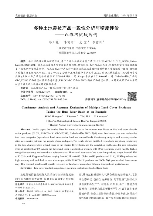
多种土地覆被产品一致性分析与精度评价——以淮河流域为例邵正艳1李南南2尤慧1李鑫川2(1淮安市气象局,江苏淮安223003;2淮阴师范学院,江苏淮安223300)摘要本文以淮河流域为研究区域,基于5种土地覆被分类产品(CLCD、ESACCI-LC、GLC_FCS30、Globe-Land30、MCD12Q1),将各土地覆被类型重分类为农用地、建设用地、未利用地三大类,从面积和空间两方面进行了一致性分析与精度评价。
结果表明,5种产品对于淮河流域土地覆被的类型特征具有较强的一致性,面积估算的相关性系数均大于0.9。
在3种30m分辨率土地覆被分类产品中,CLCD的识别精度最高,以此作为参考数据;其他4种产品总体精度在92.37%~95.53%之间,Kappa系数在0.523~0.695之间,GlobeLand30产品与GLC_FCS30产品精度较高且各有优势,ESACCI-LC产品和MCD12Q1产品精度较低。
该研究成果可以为不同时空尺度上的土地覆被研究提供参考。
关键词土地覆被产品;一致性;精度评价;淮河流域中图分类号F301.2;TP79文献标识码A文章编号1007-5739(2024)07-0170-06DOI:10.3969/j.issn.1007-5739.2024.07.040开放科学(资源服务)标识码(OSID):Consistency Analysis and Accuracy Evaluation of Multiple Land Cover Products:Taking the Huai River Basin as an ExampleSHAO Zhengyan1LI Nannan2YOU Hui1LI Xinchuan2(1Huai'an Meteorological Bureau,Huai'an Jiangsu223003;2Huaiyin Normal University,Huai'an Jiangsu223300)Abstract In this paper,the Huaihe River Basin was taken as the research area.Based on five land cover classifi-cation products(CLCD,ESACCI-LC,GLC-FCS30,GlobeLand30,MCD12Q1),each land cover type was reclassified into three categories(agricultural land,construction land and unused land).Consistency analysis and accuracy evalu-ation were carried out from two aspects of area and space.The results showed that the five products had strong consistency in the type characteristics of land cover in the Huaihe River Basin,and the correlation coefficients for area estimation were all greater than0.9.Among the three land cover classification products with30m resolution,CLCD had the highest recognition accuracy and served as a reference data.The overall accuracy of the other four products ranged from92.37% to95.53%,with Kappa coefficients ranging from0.523to0.695.GlobeLand30products and GLC_FCS30products had high accuracy and each had its own advantages,while ESACCI-LC products and MCD12Q1products had lower accu-racy.This research result could provide reference for land cover research at different temporal and spatial scales.Keywords land cover product;consistency;accuracy evaluation;Huaihe River Basin土地覆被信息是理解人类活动与全球变化复杂的交互作用的重要途径,同时也是众多生态系统模型、陆面过程模型和大气耦合模型的基础输入,它影响生态系统,包括生物多样性,调节温室气体排放以及收获和再生产[1]。
基于LandsatOLI数据的青岛市土地利用分类和植被覆盖度反演

基于LandsatOLI数据的青岛市⼟地利⽤分类和植被覆盖度反演Geomatics Science and Technology 测绘科学技术, 2019, 7(3), 132-138Published Online July 2019 in Hans. /doc/249e38125ebfc77da26925c52cc58bd630869317.html/journal/gsthttps:///doc/249e38125ebfc77da26925c52cc58bd630869317.html /10.12677/gst.2019.73019Land Use Classification and VegetationCoverage Inversion Based on Landsat OLIData in QingdaoYanzhen Liu, Yang Liu, Jia GuoShandong University of Science and Technology, Qingdao ShandongReceived: Jul. 4th, 2019; accepted: Jul. 17th, 2019; published: Jul. 24th, 2019AbstractHierarchical classification method is a method to obtain classification rules by mining spatial data information, and vegetation coverage is an important parameter to characterize surface vegeta-tion coverage. In this paper, based on the 2017 Landsat OLI image data of Qingdao city, land cover in the study area was classified and studied by stratified classification method. First of all, by making the necessary data preprocessing, the spectral characteristics of the image in the study area are analyzed and the image of NDVI, NDWI, NDBI index are calculated, and by using the strati-fied classification method we classify the land use in the research area. According to the results of land use classification and vegetation coverage inversion in the study area, it is advantageous to the planning of land utilization in Qingdao form, and it is of great importance to protect and im-prove the ecological environment of Qingdao and to plan the direction of urban development scientifically and reasonably.KeywordsLandsat OLI Data, Land Use Classification, Hierarchical Classification, Vegetation Coverage基于Landsat OLI数据的青岛市⼟地利⽤分类和植被覆盖度反演刘艳祯,刘杨,郭佳⼭东科技⼤学,⼭东青岛收稿⽇期:2019年7⽉4⽇;录⽤⽇期:2019年7⽉17⽇;发布⽇期:2019年7⽉24⽇刘艳祯等摘要分层分类⽅法是⼀种通过挖掘空间数据信息来获取分类规则的⽅法,植被覆盖度则是刻画地表植被覆盖的重要参数。
英语国家概况考点及要点

英语国家概况考点及要点The United KingdomWhat is the geographical position of the uk?It is marked by latitude 50`N in southern England and by latitude 60’ across the Shetland islands off the northwest coast of Scotland. The distance from the southern coast of England to the most northern point of the Scottish mainland is 995km, and the English east coast and welsh west coast are 483km apart. With an area of 242,524 square km.Could you give examples of important rivers in the uk? What is the lake district famous for in British literary history.1.The largest river, the seven, is 338 km in length, beginning in Wales, emptying into the Atlantic Ocean.2.The second largest but most important river is the Thames.3. In Scotland, the Clyde lake and the forth.4.in Northern Ireland, the lagan, the Bann, and the foyle. Lake District, located in the cumbrian mountains of northwest England, comprises 15 major beautiful lakes and has become a popular tourist destination. This district is attractive also because of its association with the lake poet s, who settled there in the early 1800s. What influences the climate in the uk? What are its features with respect to temperature rainfall and sunshine?The moist and mild westerly wind from the Atlantic Ocean. The warm drift of the Gulf Stream around the land. Smallness of the British Isles and its inlet-filled coastal configuration.Rainfall: is fairly well distributed throughout the year, with February to march being the driest period and October to January, the wettest. Temperature: rarely lower than 0`c in winteror higher than 32`c in summer. July and august are normally the warmest months In England. December to February is often cold, wet and windy. Sunshine: the uk is not a very sunny country. In summer, average daily sunshine varies from 5 hours in northern Scotland to 8 hours on the Isle of Wight in the south. In winter, 1 hour in northern Scotland, 2 hours on the south coast of England.How does the weather in the uk affect British life.The uk unique climate pattern inevitably results in a changeable and often unpredictable weather. This provides a constant topic of daily conversation for the Britons and it is believed that this changeability of weather is a conditioning factor of the national character that has helped the British become more adaptable.Uk is made up of: England (London), Scotland (Edinburgh), Wales (Cardiff), northern Ireland (Belfast). London is located on the bank of the river Thames in southeast England.The uk cost ling is very long, about 8000km.What patterns of settlement and immigration has the uk demonstrated in history?The United Kingdom has a multinational and multi-ethnic society where its people have diverse origins in every continent of the world. Its contemporary population is predominantly of English, welsh, Scottish and northern Irish stock, who have derived from varied settlement internal migration and assimilation in history.Is it correct to describe contemporary British society as”multi-ethnic” and “multinational” if so, why?The British are often regarded as a “mixed”people, meaning that they are products of waves of invasion and immigration from different ethnic groups in the course of history.Their ethnic origins have been complicated by intermarriage and relocation.They are: 1. Neolithic Iberians (in the Bronze Age) 2. Celtic tribes (between 600 bc and 43 ad, bringing in an iron age civilization and two languages that became the later Gaelic and welsh) 3. Romans (55 bc,) 4. Germanic (5th to 7th century, come to constitute Britain’s present predominant stock, their language became the foundation of the basic, short, everyday words in modern English) 5. Scandinavians(Vikings, 8th to 9th , subdued and integrated by the Anglo-Saxon agricultural and Christian culture.) 6. French Normans.( in 1066) meaning: Celtic languages are still used to some extent and Celtic culture is still celebrated. Affected the developing fabric of British life and formed the first foundations of the modern state. This mixture, increased by later immigration, has produced the present ethnic and national diversity in Britain.Immigrations: Jewish moneylenders, 1330, Dutch and Flemish, helping build the textile trade in England. Others, including gypsies, enslaved blacks and a further wave of Jews. In 16th and 17th, refutes from Europe, such as Dutch Protestants and French Huguenots that added to Britain’s agricultural population. 19th, countryside to urban centres, from Wales, Scotland and Ireland to England. 1840s, Irish people moved to Britain because of potato famine. Meaning: in history, the multicultural communities have helped build today’s vibrant uk and contributed to its economic and social development. With its range and unique mix of cultural identities and heritages, is seen to have defined and added cultural value to the contemporary uk. But, inequality and discrimination do exist in Britain society because of the differences in religion, race, andcultural habits, particularly at times of economic stagnation. As a consequence, it seems that ethnic divisions and tensions will have increasing rather than diminishing significance for British life.How has English language evolved in history? Why is it said that it is important to the uk`s class structure? Class structure: 1. upper-middle class 2. Middle class 3. lower middle class 4. Skilled working class 5. Semi-skilled and unskilled working class 6. Those at the lowest level of subsistence.Who were the main foreign invaders of Britain at different times in British history? What contributions have they respectively made to the British culture, or what impacts have they had?1.Early Settlers (5000BC-55BC)early man came from the European continent, stone circles and tools appeared all over the British Isles in the Neolithic Age from around 4400 bc. Famous sites of Stonehenge and silbury hill.2.the celts invaded from central Europe by 500 BC. They introduced 2 important changes: the beginning of the Iron Age and the building of hill forts.II. Roman Britain (55BC-410AD)罗马人统治时期的英国(公元前55年-410年)1.British recorded history begins with the Roman invasion. In 55BC and 54BC, Julius Caesar, a Roman general, invaded Britain twice.2. Roman's influence on Britain.The Roman built many towns, road, baths, temples and buildings. They make good use of Britain's natural resources. They also brought the new religion, Christianity, to Britain.罗马人修建了许多城镇网,道路,澡堂,庙宇和其他建筑物。
Ranking Continuous Probabilistic Datasets

Jian Li
University of Maryland, College Park
Amol Deshpande
University of Maryland, College Park
lijian@
-2-1 0 0.8
1
2 -2-1 0 1 2
Red
0.6 0.4 0.2 0.0 -2-10 1 2
Gaussian(0, 0.6) Cubic Spline Approx.
$4000-5000
Poor-Fair 21
22
(i)
(ii)
1.
INTRODUCTION
Ranking and top-k query processing are important tools in decisionmaking and analysis over large datasets and have been a subject of active research for many years in the database community [14]. In recent years, the rapid increase in the amount of uncertain data in a variety of application domains has led to much work on efficiently ranking uncertain datasets. The need for ranking or top-k processing in presence of uncertainty arises in many application domains. In financial applications, we may want to choose the best stocks in which to invest, given their expected performance in the future (which is uncertain at best). In data integration and information extraction over the web, uncertainty may arise because of incomplete data or lack of confidence in the extractions, and these uncertainties must be taken into account when returning the “best” answers for a user query (Figure 1(i)). In sensor networks or scientific databases, we may not know the “true” values of the physical properties being
审计学:一种整合方法阿伦斯英文版第12版课后答案Chapter15SolutionsManual
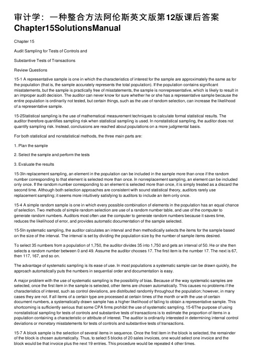
审计学:⼀种整合⽅法阿伦斯英⽂版第12版课后答案Chapter15SolutionsManualChapter 15Audit Sampling for Tests of Controls andSubstantive Tests of TransactionsReview Questions15-1 A representative sample is one in which the characteristics of interest for the sample are approximately the same as for the population (that is, the sample accurately represents the total population). If the population contains significant misstatements, but the sample is practically free of misstatements, the sample is nonrepresentative, which is likely to result in an improper audit decision. The auditor can never know for sure whether he or she has a representative sample because the entire population is ordinarily not tested, but certain things, such as the use of random selection, can increase the likelihood of a representative sample.15-2Statistical sampling is the use of mathematical measurement techniques to calculate formal statistical results. The auditor therefore quantifies sampling risk when statistical sampling is used. In nonstatistical sampling, the auditor does not quantify sampling risk. Instead, conclusions are reached about populations on a more judgmental basis.For both statistical and nonstatistical methods, the three main parts are:1. Plan the sample2. Select the sample and perform the tests3. Evaluate the results15-3In replacement sampling, an element in the population can be included in the sample more than once if the random number corresponding to that element is selected more than once. In nonreplacement sampling, an element can be included only once. If the random number corresponding to an element is selected more than once, it is simply treated as a discard the second time. Although both selection approaches are consistent with sound statistical theory, auditors rarely use replacement sampling; it seems more intuitively satisfying to auditors to include an item only once.15-4 A simple random sample is one in which every possible combination of elements in the population has an equal chance of selection. Two methods of simple random selection are use of a random number table, and use of the computer to generate random numbers. Auditors most often use the computer to generate random numbers because it saves time, reduces the likelihood of error, and provides automatic documentation of the sample selected.15-5In systematic sampling, the auditor calculates an interval and then methodically selects the items for the sample based on the size of the interval. The interval is set by dividing the population size by the number of sample items desired.To select 35 numbers from a population of 1,750, the auditor divides 35 into 1,750 and gets an interval of 50. He or she then selects a random number between 0 and 49. Assume the auditor chooses 17. The first item is the number 17. The next is 67, then 117, 167, and so on.The advantage of systematic sampling is its ease of use. In most populations a systematic sample can be drawn quickly, the approach automatically puts the numbers in sequential order and documentation is easy.A major problem with the use of systematic sampling is the possibility of bias. Because of the way systematic samples are selected, once the first item in the sample is selected, other items are chosen automatically. This causes no problems if the characteristics of interest, such as control deviations, are distributed randomly throughout the population; however, in many cases they are not. If all items of a certain type are processed at certain times of the month or with the use of certain document numbers, a systematically drawn sample has a higher likelihood of failing to obtain a representative sample. This shortcoming is sufficiently serious that some CPA firms prohibit the use of systematic sampling. 15-6The purpose of using nonstatistical sampling for tests of controls and substantive tests of transactions is to estimate the proportion of items in a population containing a characteristic or attribute of interest. The auditor is ordinarily interested in determining internal control deviations or monetary misstatements for tests of controls and substantive tests of transactions.15-7 A block sample is the selection of several items in sequence. Once the first item in the block is selected, the remainder of the block is chosen automatically. Thus, to select 5 blocks of 20 sales invoices, one would select one invoice and the block would be that invoice plus the next 19 entries. This procedure would be repeated 4 other times.15-8 The terms below are defined as follows:15-8 (continued)15-9The sampling unit is the population item from which the auditor selects sample items. The major consideration in defining the sampling unit is making it consistent with the objectives of the audit tests. Thus, the definition of the population and the planned audit procedures usually dictate the appropriate sampling unit.The sampling unit for verifying the occurrence of recorded sales would be the entries in the sales journal since this is the document the auditor wishes to validate. The sampling unit for testing the possibility of omitted sales is the shipping document from which sales are recorded because the failure to bill a shipment is the exception condition of interest to the auditor.15-10 The tolerable exception rate (TER) represents the exception rate that the auditor will permit in the population and still be willing to use the assessed control risk and/or the amount of monetary misstatements in the transactions established during planning. TER is determined by choice of the auditor on the basis of his or her professional judgment.The computed upper exception rate (CUER) is the highest estimated exception rate in the population, at a given ARACR. For nonstatistical sampling, CUER is determined by adding an estimate of sampling error to the SER (sample exception rate). For statistical sampling, CUER is determined by using a statistical sampling table after the auditor has completed the audit testing and therefore knows the number of exceptions in the sample.15-11 Sampling error is an inherent part of sampling that results from testing less than the entire population. Sampling error simply means that the sample is not perfectly representative of the entire population.Nonsampling error occurs when audit tests do not uncover errors that exist in the sample. Nonsampling error can result from:1. The auditor's failure to recognize exceptions, or2. Inappropriate or ineffective audit procedures.There are two ways to reduce sampling risk:1. Increase sample size.2. Use an appropriate method of selecting sample items from thepopulation.Careful design of audit procedures and proper supervision and review are ways to reduce nonsampling risk.15-12 An attribute is the definition of the characteristic being tested and the exception conditions whenever audit sampling is used. The attributes of interest are determined directly from the audit program.15-13 An attribute is the characteristic being tested for in a population. An exception occurs when the attribute being tested for is absent. The exception for the audit procedure, the duplicate sales invoice has been initialed indicating the performance of internal verification, is the lack of initials on duplicate sales invoices.15-14 Tolerable exception rate is the result of an auditor's judgment. The suitable TER is a question of materiality and is therefore affected by both the definition and the importance of the attribute in the audit plan.The sample size for a TER of 6% would be smaller than that for a TER of 3%, all other factors being equal.15-15 The appropriate ARACR is a decision the auditor must make using professional judgment. The degree to which the auditor wishes to reduce assessed control risk below the maximum is the major factor determining the auditor's ARACR.The auditor will choose a smaller sample size for an ARACR of 10% than would be used if the risk were 5%, all other factors being equal.15-16 The relationship between sample size and the four factors determining sample size are as follows:a. As the ARACR increases, the required sample size decreases.b. As the population size increases, the required sample size isnormally unchanged, or may increase slightly.c. As the TER increases, the sample size decreases.d. As the EPER increases, the required sample size increases.15-17 In this situation, the SER is 3%, the sample size is 100 and the ARACR is 5%. From the 5% ARACR table (Table 15-9) then, the CUER is 7.6%. This means that the auditor can state with a 5% risk of being wrong that the true population exception rate does not exceed 7.6%.15-18 Analysis of exceptions is the investigation of individual exceptions to determine the cause of the breakdown in internal control. Such analysis is important because by discovering the nature and causes of individual exceptions, the auditor can more effectively evaluate the effectiveness of internal control. The analysis attempts to tell the "why" and "how" of the exceptions after the auditor already knows how many and what types of exceptions have occurred.15-19 When the CUER exceeds the TER, the auditor may do one or more of the following:1. Revise the TER or the ARACR. This alternative should be followed onlywhen the auditor has concluded that the original specifications weretoo conservative, and when he or she is willing to accept the riskassociated with the higher specifications.2. Expand the sample size. This alternative should be followed whenthe auditor expects the additional benefits to exceed the additionalcosts, that is, the auditor believes that the sample tested was notrepresentative of the population.3. Revise assessed control risk upward. This is likely to increasesubstantive procedures. Revising assessed control risk may bedone if 1 or 2 is not practical and additional substantive proceduresare possible.4. Write a letter to management. This action should be done inconjunction with each of the three alternatives above. Managementshould always be informed when its internal controls are notoperating effectively. If a deficiency in internal control is consideredto be a significant deficiency in the design or operation of internalcontrol, professional standards require the auditor to communicatethe significant deficiency to the audit committee or its equivalent inwriting. If the client is a publicly traded company, the auditor mustevaluate the deficiency to determine the impact on the auditor’sreport on internal control over financial reporting. If the deficiency isdeemed to be a material weakness, the auditor’s report on internalcontrol would contain an adverse opinion.15-20 Random (probabilistic) selection is a part of statistical sampling, but it is not, by itself, statistical measurement. To have statistical measurement, it is necessary to mathematically generalize from the sample to the population.Probabilistic selection must be used if the sample is to be evaluated statistically, although it is also acceptable to use probabilistic selection with a nonstatistical evaluation. If nonprobabilistic selection is used, nonstatistical evaluation must be used.15-21 The decisions the auditor must make in using attributes sampling are: What are the objectives of the audit test? Does audit sampling apply?What attributes are to be tested and what exception conditions are identified?What is the population?What is the sampling unit?What should the TER be?What should the ARACR be?What is the EPER?What generalizations can be made from the sample to thepopulation?What are the causes of the individual exceptions?Is the population acceptable?15-21 (continued)In making the above decisions, the following should be considered: The individual situation.Time and budget constraints.The availability of additional substantive procedures.The professional judgment of the auditor.Multiple Choice Questions From CPA Examinations15-22 a. (1) b. (3) c. (2) d. (4)15-23 a. (1) b. (3) c. (4) d. (4)15-24 a. (4) b. (3) c. (1) d. (2)Discussion Questions and Problems15-25a.An example random sampling plan prepared in Excel (P1525.xls) is available on the Companion Website and on the Instructor’s Resource CD-ROM, which is available upon request. The command for selecting the random number can be entered directly onto the spreadsheet, or can be selected from the function menu (math & trig) functions. It may be necessary to add the analysis tool pack to access the RANDBETWEEN function. Once the formula is entered, it can be copied down to select additional random numbers. When a pair of random numbers is required, the formula for the first random number can be entered in the first column, and the formula for the second random number can be entered in the second column.a. First five numbers using systematic selection:Using systematic selection, the definition of the sampling unit for determining the selection interval for population 3 is the total number of lines in the population. The length of the interval is rounded down to ensure that all line numbers selected are within the defined population.15-26a. To test whether shipments have been billed, a sample of warehouse removal slips should be selected and examined to see ifthey have the proper sales invoice attached. The sampling unit willtherefore be the warehouse removal slip.b. Attributes sampling method: Assuming the auditor is willing to accept a TER of 3% at a 10% ARACR, expecting no exceptions in the sample, the appropriate sample size would be 76, determined from Table 15-8.Nonstatistical sampling method: There is no one right answer to this question because the sample size is determined using professional judgment. Due to the relatively small TER (3%), the sample size should not be small. It will most likely be similar in size to the sample chosen by the statistical method.c. Systematic sample selection:22839 = Population size of warehouse removal slips(37521-14682).76 = Sample size using statistical sampling (students’answers will vary if nonstatistical sampling wasused in part b.300 = Interval (22839/76) if statistical sampling is used (students’ answers will vary if nonstatisticalsampling was used in part b).14825 = Random starting point.Select warehouse removal slip 14825 and every 300th warehouse removal slip after (15125, 15425, etc.)Computer generation of random numbers using Excel (P1526.xls): =RANDBETWEEN(14682,37521)The command for selecting the random number can be entered directly onto the spreadsheet, or can be selected from the function menu (math & trig) functions. It may be necessary to add the analysis tool pack to access the RANDBETWEEN function. Once the formula is entered, it can be copied down to select additional random numbers.d. Other audit procedures that could be performed are:1. Test extensions on attached sales invoices for clerical accuracy. (Accuracy)2. Test time delay between warehouse removal slip date and billing date for timeliness of billing. (Timing)3. Trace entries into perpetual inventory records to determinethat inventory is properly relieved for shipments. (Postingand summarization)15-26 (continued)e. The test performed in part c cannot be used to test for occurrenceof sales because the auditor already knows that inventory wasshipped for these sales. To test for occurrence of sales, the salesinvoice entry in the sales journal is the sampling unit. Since thesales invoice numbers are not identical to the warehouse removalslips it would be improper to use the same sample.15-27a. It would be appropriate to use attributes sampling for all audit procedures except audit procedure 1. Procedure 1 is an analyticalprocedure for which the auditor is doing a 100% review of the entirecash receipts journal.b. The appropriate sampling unit for audit procedures 2-5 is a line item,or the date the prelisting of cash receipts is prepared. The primaryemphasis in the test is the completeness objective and auditprocedure 2 indicates there is a prelisting of cash receipts. All otherprocedures can be performed efficiently and effectively by using theprelisting.c. The attributes for testing are as follows:d. The sample sizes for each attribute are as follows:15-28a. Because the sample sizes under nonstatistical sampling are determined using auditor judgment, students’ answers to thisquestion will vary. They will most likely be similar to the samplesizes chosen using attributes sampling in part b. The importantpoint to remember is that the sample sizes chosen should reflectthe changes in the four factors (ARACR, TER, EPER, andpopulation size). The sample sizes should have fairly predictablerelationships, given the changes in the four factors. The followingreflects some of the relationships that should exist in student’ssample size decisions:SAMPLE SIZE EXPLANATION1. 90 Given2. > Column 1 Decrease in ARACR3. > Column 2 Decrease in TER4. > Column 1 Decrease in ARACR (column 4 is thesame as column 2, with a smallerpopulation size)5. < Column 1 Increase in TER-EPER6. < Column 5 Decrease in EPER7. > Columns 3 & 4 Decrease in TER-EPERb. Using the attributes sampling table in Table 15-8, the sample sizesfor columns 1-7 are:1. 882. 1273. 1814. 1275. 256. 187. 149c.d. The difference in the sample size for columns 3 and 6 result from the larger ARACR and larger TER in column 6. The extremely large TER is the major factor causing the difference.e. The greatest effect on the sample size is the difference between TER and EPER. For columns 3 and 7, the differences between the TER and EPER were 3% and 2% respectively. Those two also had the highest sample size. Where the difference between TER and EPER was great, such as columns 5 and 6, the required sample size was extremely small.Population size had a relatively small effect on sample size.The difference in population size in columns 2 and 4 was 99,000 items, but the increase in sample size for the larger population was marginal (actually the sample sizes were the same using the attributes sampling table).f. The sample size is referred to as the initial sample size because it is based on an estimate of the SER. The actual sample must be evaluated before it is possible to know whether the sample is sufficiently large to achieve the objectives of the test.15-29 a.* Students’ answers as to whether the allowance for sampling error risk is sufficient will vary, depending on their judgment. However, they should recognize the effect that lower sample sizes have on the allowance for sampling risk in situations 3, 5 and 8.b. Using the attributes sampling table in Table 15-9, the CUERs forcolumns 1-8 are:1. 4.0%2. 4.6%3. 9.2%4. 4.6%5. 6.2%6. 16.4%7. 3.0%8. 11.3%c.d. The factor that appears to have the greatest effect is the number ofexceptions found in the sample compared to sample size. For example, in columns 5 and 6, the increase from 2% to 10% SER dramatically increased the CUER. Population size appears to have the least effect. For example, in columns 2 and 4, the CUER was the same using the attributes sampling table even though the population in column 4 was 10 times larger.e. The CUER represents the results of the actual sample whereas theTER represents what the auditor will allow. They must be compared to determine whether or not the population is acceptable.15-30a. and b. The sample sizes and CUERs are shown in the following table:a. The auditor selected a sample size smaller than that determinedfrom the tables in populations 1 and 3. The effect of selecting asmaller sample size than the initial sample size required from thetable is the increased likelihood of having the CUER exceed theTER. If a larger sample size is selected, the result may be a samplesize larger than needed to satisfy TER. That results in excess auditcost. Ultimately, however, the comparison of CUER to TERdetermines whether the sample size was too large or too small.b. The SER and CUER are shown in columns 4 and 5 in thepreceding table.c. The population results are unacceptable for populations 1, 4, and 6.In each of those cases, the CUER exceeds TER.The auditor's options are to change TER or ARACR, increase the sample size, or perform other substantive tests to determine whether there are actually material misstatements in thepopulation. An increase in sample size may be worthwhile inpopulation 1 because the CUER exceeds TER by only a smallamount. Increasing sample size would not likely result in improvedresults for either population 4 or 6 because the CUER exceedsTER by a large amount.d. Analysis of exceptions is necessary even when the population isacceptable because the auditor wants to determine the nature andcause of all exceptions. If, for example, the auditor determines thata misstatement was intentional, additional action would be requiredeven if the CUER were less than TER.15-30 (Continued)e.15-31 a. The actual allowance for sampling risk is shown in the following table:b. The CUER is higher for attribute 1 than attribute 2 because the sample sizeis smaller for attribute 1, resulting in a larger allowance for sampling risk.c. The CUER is higher for attribute 3 than attribute 1 because the auditorselected a lower ARACR. This resulted in a larger allowance for sampling risk to achieve the lower ARACR.d. If the auditor increases the sample size for attribute 4 by 50 items and findsno additional exceptions, the CUER is 5.1% (sample size of 150 and three exceptions). If the auditor finds one exception in the additional items, the CUER is 6.0% (sample size of 150, four exceptions). With a TER of 6%, the sample results will be acceptable if one or no exceptions are found in the additional 50 items. This would require a lower SER in the additional sample than the SER in the original sample of 3.0 percent. Whether a lower rate of exception is likely in the additional sample depends on the rate of exception the auditor expected in designing the sample, and whether the auditor believe the original sample to be representative.15-32a. The following shows which are exceptions and why:b. It is inappropriate to set a single acceptable tolerable exception rate and estimated population exception rate for the combined exceptions because each attribute has a different significance tothe auditor and should be considered separately in analyzing the results of the test.c. The CUER assuming a 5% ARACR for each attribute and a sample size of 150 is as follows:15-32 (continued)d.*Students’ answers will most likely vary for this attribute.e. For each exception, the auditor should check with the controller todetermine an explanation for the cause. In addition, the appropriateanalysis for each type of exception is as follows:15-33a. Attributes sampling approach: The test of control attribute had a 6% SER and a CUER of 12.9%. The substantive test of transactionsattribute has SER of 0% and a CUER of 4.6%.Nonstatistical sampling approach: As in the attributes samplingapproach, the SERs for the test of control and the substantive testof transactions are 6% and 0%, respectively. Students’ estimates ofthe CUERs for the two tests will vary, but will probably be similar tothe CUERs calculated under the attributes sampling approach.b. Attributes sampling approach: TER is 5%. CUERs are 12.9% and4.6%. Therefore, only the substantive test of transactions resultsare satisfactory.Nonstatistical sampling approach: Because the SER for the test ofcontrol is greater than the TER of 5%, the results are clearly notacceptable. Students’ estimates for CUER for the test of controlshould be greater than the SER of 6%. For the substantive test oftransactions, the SER is 0%. It is unlikely that students will estimateCUER for this test greater than 5%, so the results are acceptablefor the substantive test of transactions.c. If the CUER exceeds the TER, the auditor may:1. Revise the TER if he or she thinks the original specificationswere too conservative.2. Expand the sample size if cost permits.3. Alter the substantive procedures if possible.4. Write a letter to management in conjunction with each of theabove to inform management of a deficiency in their internalcontrols. If the client is a publicly traded company, theauditor must evaluate the deficiency to determine the impacton the auditor’s report on internal control over financialreporting. If the deficiency is deemed to be a materialweakness, the auditor’s report on internal control wouldcontain an adverse opinion.In this case, the auditor has evidence that the test of control procedures are not effective, but no exceptions in the sample resulted because of the breakdown. An expansion of the attributestest does not seem advisable and therefore, the auditor shouldprobably expand confirmation of accounts receivable tests. Inaddition, he or she should write a letter to management to informthem of the control breakdown.d. Although misstatements are more likely when controls are noteffective, control deviations do not necessarily result in actualmisstatements. These control deviations involved a lack ofindication of internal verification of pricing, extensions and footingsof invoices. The deviations will not result in actual errors if pricing,extensions and footings were initially correctly calculated, or if theindividual responsible for internal verification performed theprocedure but did not document that it was performed.e. In this case, we want to find out why some invoices are notinternally verified. Possible reasons are incompetence,carelessness, regular clerk on vacation, etc. It is desirable to isolatethe exceptions to certain clerks, time periods or types of invoices.Case15-34a. Audit sampling could be conveniently used for procedures 3 and 4 since each is to be performed on a sample of the population.b. The most appropriate sampling unit for conducting most of the auditsampling tests is the shipping document because most of the testsare related to procedure 4. Following the instructions of the auditprogram, however, the auditor would use sales journal entries asthe sampling unit for step 3 and shipping document numbers forstep 4. Using shipping document numbers, rather than thedocuments themselves, allows the auditor to test the numericalcontrol over shipping documents, as well as to test for unrecordedsales. The selection of numbers will lead to a sample of actualshipping documents upon which tests will be performed.。
- 1、下载文档前请自行甄别文档内容的完整性,平台不提供额外的编辑、内容补充、找答案等附加服务。
- 2、"仅部分预览"的文档,不可在线预览部分如存在完整性等问题,可反馈申请退款(可完整预览的文档不适用该条件!)。
- 3、如文档侵犯您的权益,请联系客服反馈,我们会尽快为您处理(人工客服工作时间:9:00-18:30)。
a rXiv:alg-ge o m/94806v124Aug1994On Landsberg’s criterion for complete intersections S.L’vovsky ∗August 24,1994Introduction In his preprint [1],ndsberg introduces an elementary characterization of complete intersections (Proposition 1.2in [1]).The proof of this proposition uses the method of moving frames.The aim of this note is to present an elementary proof of Landsberg’s criterion that is valid over any ground field.1Notation and statement of results Let k be an algebraically closed field and P N =Proj k [T 0,...,T N ]the N -dimensional projective space over k .If F is a homogeneous polynomial in T 0,...,T N ,we will denote by Z (F )⊂P N the hypersurface defined by F .If F is a homogeneous polynomial and x =(x 0:...:x N )∈P N ,put d x F =(∂F/∂T 0(z ),...,∂F/∂T N (z ))∈k N +1(actually d x F depends on the choice of homogeneous coordinates for x ;this abuse of notation should not lead to confu-sion).If x ∈X ,where X ⊂P N is a projective variety,then T x X ⊂P N denotes the embedded Zariski tangent space to X at x .If X ⊂P N is a projective variety,then its ideal sheaf will be denoted byI X ⊂O P N and its homogeneous ideal by I X ⊂k [T 0,...,T N ].We will say that a hypersurface Y =Z (F )trivially contains X iffF = G i F i ,where G i ’s and F i ’s are homogeneous polynomials,F i vanish on X for all i ,and deg F i <deg F for all i .If Y trivially contains X ,then Y ⊃X .We will say that a hypersurface W non-trivially contains X iffW contains X ,but not trivially.The following proposition is a slight reformulation of Landsberg’s criterion (cf.[1,Proposition 1.2]):Proposition 1.1For a projective variety X ⊂P N ,the following conditions are equivalent:(i)X is a complete intersection.(ii)There exists a smooth point x∈X having the following property:any hypersurface W⊂P N that non-trivially contains X must be smooth at x.(iii)For any smooth point x∈X and any hypersurface W that non-trivially contains X,W is smooth at x.(iv)For any smooth point x∈X and any hypersurface W that non-trivially contains X,T x W cannot contain an intersection i T x W i,where each W i is a hypersurface s.t.W i⊃X and deg W i<deg W(it is understood that the intersection of an empty family of tangent spaces is the entire P N).2ProofsFor the sequel we need two lemmas.Lemma2.1Let F1,...,F r be homogeneous polynomials over k in T0,...,T N. Assume that x=(x0:...:x N)∈P N is their common zero and that the vectors d x F1,...,d x F r are linearly dependent.Then one of the following alternatives holds:1.There is j∈[1;r]s.t.F j belongs to the ideal in k[T0,...,T N]generated byF i’s with i=j.2.There are homogeneous polynomials˜F0,...,˜F N s.t.the ideals(F0,...,F N)and(˜F0,...,˜F N)coincide,deg˜F i=deg F i for all i,and d x˜F j=0for some j.Proof.Let the shortest linear relation among d x F j’s have the formλ1d x F1+···+λs d x F s=0,whereλj=0for all j.Reordering F j’s if necessary,we may assume that deg F1≤deg F2≤···≤deg F s.Let t be such a number that deg F t=deg F s and deg F t−1<deg F s(if deg F1=deg F s,set t=1).If the polynomials F t,...,F s are linearly dependent,then it is clear that one of them lies in the ideal generated by the others and there is nothing more to prove.Assume from now on that F t,F t+1,...,F s are linearly independent. Then there exists an index j∈[t;s]and numbersµi,where i∈[t;s]s.t.µi F i+µj(λt F t+···+λs F s).(1)F j=i∈[t;s]\{j}For each i∈[1;t−1],choose a homogeneous polynomial G i s.t.deg G i= deg F s−deg F i and G i(x0,...,x N)=λi,and set˜F= i<t G i F i+ i≥tλi F i.(2)j2If˜F j=0,then F s∈(F1,...,F s−1)and thefirst alternative holds.Otherwise, deg˜F j=deg F j,d x˜F j=0by virtue of(2),and it follows from(1)and(2)thatµi F i+µj˜F j−µj i<t G i F i,F j=i∈[t;s]\{j}whence(F1,...,F j−1,˜F j,F j+1,...,F s)=(F1,...,F s).Hence in this case the second alternative holds,and we are done.The second lemma belongs to folklore.To state this lemma,let us introduce some notation.Denote by S the set of sequences of non-negative integersδ= (δ1,δ2,...)s.t.δM=0for all M≫0.Ifδ,η∈S,we will writeδ≻ηiffthere is an integer i s.t.δi>ηi andδj=ηj for all j>i.Lemma2.2Any sequenceδ1≻δ2≻···must terminate.Proof.For anyδ∈S,set n(δ)=max{j:δj=0},ℓ(δ)=δn(δ)>0.Ifδ≻ηand n(δ)=n(η),thenℓ(δ)≥ℓ(η).Let us prove the lemma by induction on n(δ1).If n(δ1)≤1,the result is evident.Assuming that the lemma is true whenever n(δ1)<m,suppose that there is an infinite sequenceδ1≻δ2≻...with n(δ1)= m.If n(δj)<n(δ1)for some j,we arrive at a contradiction by the induction hypothesis.Hence,n(δj)=n(δ1)=m for all j andℓ(δ1)≥ℓ(δ2)≥ 0Thus there exists an integer N s.tℓ(δj)is connstant for j≥N.For any j≥N, denote byδ′j∈S a sequence that is obtained fromδj by replacing its last positive term by zero.It is clear thatδ′N≻δ′N+1≻···,and this sequence is infinite by our assumption.This is again impossible by the induction hypothesis since n(δ′j)<n(δj)=m,whence the lemma.Proof of(ii)⇒(i).Put a=N−dim X.Let(F1,...,F r)be a system of(homogeneous)generators of I X.To any such system assign a sequence δ(F1,...,F r)∈S,whereδ(F1,...,F r)i=#{j∈[1;r]:deg F j=i}.I claim thatif r>a,then I X=(Φ1,...,Φs),whereΦi’s are homogeneous poly-nomials s.t.δ(F1,...,F r)≻δ(Φ1,...,Φs).To prove this claim,observe that d x F1,...,d x F r are linearly dependent since X is smooth at x and r>codim X.Now Lemma2.1implies that either one of the F j’s(say,F1)can be removed without affecting I X,or I X=(˜F1,...,˜F r), where deg˜F j=deg F j for all j and d x˜F j=0for some j.In thefirst case,the requiredΦ1,...,Φs can be obtained by merely removing F1;in the second case, hypothesis(ii)shows that˜F j= t i=1G iΨi,whereΨi∈I X and degΨi<deg˜F j for all j.Replacing˜F j byΨ1,...,Ψt in the sequence˜F1,...,˜F r and putting s=r+t−1,we obtain a sequenceΦ1,...,Φs s.t.I X=(Φ1,...,Φs)and δ(˜F1,...,˜F r)≻δ(Φ1,...,Φs).Since the degrees of˜F j’s and F j’s are the same, this means thatδ(F1,...,F r)≻δ(Φ1,...,Φs)as well,and the claim is proved.3Now we canfinish the proof as follows.If r=a,then X is the complete intersection of Z(F1),...,Z(F r)and there is nothing to prove.If r>a,then by virtue of our claim we can replace the system of generators F1,...,F r by Φ1,...,Φs.Let us iterate this process.By virtue of Lemma2.2this process must terminate and by virtue of our claim this is possible only when we have found a system of exactly a generators of the ideal I X.This means that X is a complete intersection,thus completing our proof.Proof of(iv)⇒(iii)⇒(ii).Trivial.Proof of(i)⇒(iv).Let X be a complete intersection of the hypersurfaces Z(F1),...,Z(F a).Assume that a hypersurface W=Z(F),with F irreducible, non-trivially contains X and that x=(x0:...:x N)∈P N is a smooth point of X;set m=deg F.Since Z(F)⊃X and X is a complete intersection of the Z(F i)’s,we see thatF= G i F i;(3) since W contains X non-trivially,at least some of the G j’s must be non-zero constants.Reordering F j’s if necessary,we may assume that G j is a constant (hence,deg F j=m)iff1≤j≤s.Taking d x of the both parts of(3),we seethatd x F=ai=1c id x F i,where c i=0for some i∈[1;s].(4)On the other hand,assume that W i=Z(B i)with irreducible B i’s.Then the hypothesis implies that d x F is a linear combination of d x B j’s,and the fact that X is a complete intersection of Z(F t)’s and Z(B j)⊃X implies that,for each j,there is a relationB j= t>s G jt F t(5) (it suffices to sum only over t>s since for t≤s we have deg F t=deg W> deg B j).If we take d x of both parts of(5),we see that,for each j,d x B j is a linear combination of d x F t’s with t>s.Hence d x F is also a linear combination of d x F t’s with t>s.Taking into account(4)we see that d x F i’s are linearly dependent.This is,however,impossible since x is a smooth point of the comlete intersection of Z(F j)’s.This contradiction completes the proof. References[1]Landsberg,J.M.Differential-Geometric Characterizations of Complete In-tersections.Preprint,alg-geom/9407002Email address:serge@schcorr.msk.sunskcsmoscow@4。