stata命令术语
stata计算命令

stata计算命令1、使用sum命令求和sum varlist为指定变量列表求和,求出合计值。
比如,sum price 以求出所有price变量的总和。
2、使用mean命令求平均值mean varlist求取指定变量的平均值,例如:mean price 用来计算price变量的平均值。
3、使用corr命令求相关系数corr varlist为两个变量求出相关性系数,比如corr x y用来求x和y两个变量之间的相关性。
4、使用regress命令进行回归分析regress varlist对指定变量进行回归分析,比如用regress y x1 x2用来求y变量和x(1、2)变量之间的回归关系。
5、使用predict命令估计变量predict varlist根据回归模型结果估计指定变量的值,例如predict y_new x_new根据原回归模型可以估计x_new的y_new值。
6、使用describe命令查看统计量describe x这个命令可以查看指定变量的基础统计量,比如查看一列x变量的最大值、最小值、均值、方差、标准偏差、取值范围等信息。
7、使用ttest命令进行t检验ttest varlist用来对比两个组之间变量的均值,比如用ttest x y可以对比x和y变量的平均值是否有显著性差异。
8、使用test命令检验假设test test_expression用于检查两个指定表达式之间的分布差异,比如用test x1 = x2来检查x1和x2变量之间的均值是否相等。
9、使用ci命令计算置信区间ci varlist这个命令用来计算指定变量的置信区间,比如用ci x来求x变量的90%置信区间。
stata命令集

Cleardestring 变量名,replace,改变数据的格式如果数据复制进去是红色,说明是字符型,改成数值型,通过命令:gen 新变量名=real(原变量名)drop 原变量名rename 原变量名新变量名,replacesort指令是STATA数据库的维护的排序指令。
命令:tsset yeartsset指令是时间序列数据的估计命令。
如何创建一个截面数据文件?先把数据转移到stata中,然后用tsset命令。
tsset time, yearly(或者weekly、monthly、quarterly)此时,一定要保证表示时间的那一列数据(即年份)的名称为time。
时间序列数据的处理(来自百度):时间序列数据的回归主要需要注意以下几点:多重共线性(当样本量较小时,例如小于100)和序列相关性。
而且需要考察t统计值、R2(adj-R2)、F统计量、D.W.值。
首先用reg命令进行回归,例如:reg y x1 x2 x3 x4 x5,并考察D.W.值(使用estat dwatson这一命令),如果D.W.值严重远离2,那么要进行调整(调整方法如黄色底纹),直到调整到2附近,然后考察回归结果是否符合经济学含义,倘若不符合,那么要注意是否受到多重共线性的影响(通过相关系数和vif值来判断)。
在处理多重共线性时,可以用类似于处理截面数据的方法(剔除变量法),同时还要看D.W.值。
此外,还可以用差分法来处理多重共线性(此方法用得不多)。
检验DW值的命令:estat dwatson用广义差分法考虑序列相关性的命令(即调整DW值的命令):reg y x1 x2 x3 x4 x5 L.y(后面还可以运用L.y L2.y)用序列相关稳健标准误法考虑序列相关性的命令(即调整DW值的命令):reg y x1 x2 x3 x4 x5, robust考虑多重共线性的方法除了以上截面数据中用到的方法以外,还可以用差分法,然后再看vif值。
stata命令大全(全)
*
*-- F(4,373) = 855.93检验除常数项外其他解释变量的联合显著性
*-- corr(u_i, Xb)=-0.2347
*-- sigma_u, sigma_e, rho
* rho = sigma_uA2/(sigma_uA2+sigma_eA2)
*空间计量分析:SLM模型与SEM模型
*说明:STATA与Matlab结合使用。常应用于空间溢出效应(R&D)、财政 分权、地方政府公共行为等。
、常用的数据处理与作图
*指定面板格式
xtset id year(id为截面名称,year为时间名称)
xtdes /*数据特征*/
xtsum logy h /*数据统计特征*/
drop if id==2/*注意用==*/
*如何得到连续year或id编号(当完成上述操作时, 为形成panel格式,需要用egen命令)
ege n year_ new二group(year)
xtset id year_ new
**保留变量或保留观测值
keep inv /*删除变量*/
**或
keep if year==2000
dis e(sigma_u)A2/(e(sigma_u)A2+e(sigma_e)A2)
个体效应是否显著?
*F(28,373) =338.86 HO: al=a2 = a3 = a4 = a29
*Prob > F = 0.0000表明,固定效应高度显著
*---如何得到调整后的R2即adj-R2?
ereturn list
考虑中国29个省份的C-D生产函数
Stata统计分析命令
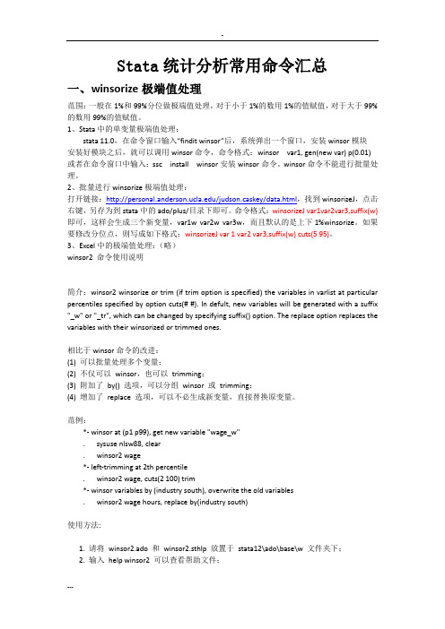
Stata统计分析常用命令汇总一、winsorize极端值处理范围:一般在1%和99%分位做极端值处理,对于小于1%的数用1%的值赋值,对于大于99%的数用99%的值赋值。
1、Stata中的单变量极端值处理:stata 11.0,在命令窗口输入“findit winsor”后,系统弹出一个窗口,安装winsor模块安装好模块之后,就可以调用winsor命令,命令格式:winsor var1, gen(new var) p(0.01) 或者在命令窗口中输入:ssc install winsor安装winsor命令。
winsor命令不能进行批量处理。
2、批量进行winsorize极端值处理:打开链接:/judson.caskey/data.html,找到winsorizeJ,点击右键,另存为到stata中的ado/plus/目录下即可。
命令格式:winsorizeJ var1var2var3,suffix(w)即可,这样会生成三个新变量,var1w var2w var3w,而且默认的是上下1%winsorize。
如果要修改分位点,则写成如下格式:winsorizeJ var 1 var2 var3,suffix(w) cuts(5 95)。
3、Excel中的极端值处理:(略)winsor2 命令使用说明简介:winsor2 winsorize or trim (if trim option is specified) the variables in varlist at particular percentiles specified by option cuts(# #). In defult, new variables will be generated with a suffix "_w" or "_tr", which can be changed by specifying suffix() option. The replace option replaces the variables with their winsorized or trimmed ones.相比于winsor命令的改进:(1) 可以批量处理多个变量;(2) 不仅可以winsor,也可以trimming;(3) 附加了by() 选项,可以分组winsor 或trimming;(4) 增加了replace 选项,可以不必生成新变量,直接替换原变量。
stata命令大全(全)

********* 面板数据计量分析与软件实现 *********说明:以下do文件相当一部分内容来自于中山大学连玉君STATA教程,感谢他的贡献。
本人做了一定的修改与筛选。
*----------面板数据模型* 1.静态面板模型:FE 和RE* 2.模型选择:FE vs POLS, RE vs POLS, FE vs RE (pols混合最小二乘估计) * 3.异方差、序列相关和截面相关检验* 4.动态面板模型(DID-GMM,SYS-GMM)* 5.面板随机前沿模型* 6.面板协整分析(FMOLS,DOLS)*** 说明:1-5均用STATA软件实现, 6用GAUSS软件实现。
* 生产效率分析(尤其指TFP):数据包络分析(DEA)与随机前沿分析(SFA)*** 说明:DEA由DEAP2.1软件实现,SFA由Frontier4.1实现,尤其后者,侧重于比较C-D与Translog生产函数,一步法与两步法的区别。
常应用于地区经济差异、FDI 溢出效应(Spillovers Effect)、工业行业效率状况等。
* 空间计量分析:SLM模型与SEM模型*说明:STATA与Matlab结合使用。
常应用于空间溢出效应(R&D)、财政分权、地方政府公共行为等。
* ---------------------------------* --------一、常用的数据处理与作图-----------* ---------------------------------* 指定面板格式xtset id year (id为截面名称,year为时间名称)xtdes /*数据特征*/xtsum logy h /*数据统计特征*/sum logy h /*数据统计特征*/*添加标签或更改变量名label var h "人力资本"rename h hum*排序sort id year /*是以STATA面板数据格式出现*/sort year id /*是以DEA格式出现*/*删除个别年份或省份drop if year<1992drop if id==2 /*注意用==*/*如何得到连续year或id编号(当完成上述操作时,year或id就不连续,为形成panel 格式,需要用egen命令)egen year_new=group(year)xtset id year_new**保留变量或保留观测值keep inv /*删除变量*/**或keep if year==2000**排序sort id year /*是以STATA面板数据格式出现sort year id /*是以DEA格式出现**长数据和宽数据的转换*长>>>宽数据reshape wide logy,i(id) j(year)*宽>>>长数据reshape logy,i(id) j(year)**追加数据(用于面板数据和时间序列)xtset id year*或者xtdestsappend,add(5) /表示在每个省份再追加5年,用于面板数据/tsset*或者tsdes.tsappend,add(8) /表示追加8年,用于时间序列/*方差分解,比如三个变量Y,X,Z都是面板格式的数据,且满足Y=X+Z,求方差var(Y),协方差Cov(X,Y)和Cov(Z,Y)bysort year:corr Y X Z,cov**生产虚拟变量*生成年份虚拟变量tab year,gen(yr)*生成省份虚拟变量tab id,gen(dum)**生成滞后项和差分项xtset id yeargen ylag=l.y /*产生一阶滞后项),同样可产生二阶滞后项*/gen ylag2=L2.ygen dy=D.y /*产生差分项*/*求出各省2000年以前的open inv的平均增长率collapse (mean) open inv if year<2000,by(id)变量排序,当变量太多,按规律排列。
stata常用命令

面板数据估计首先对面板数据进行声明:前面是截面单元,后面是时间标识:tsset company yeartsset industry year产生新的变量:gen newvar=human*lnrd产生滞后变量Gen fiscal(2)=L2.fiscal产生差分变量Gen fiscal(D)=D.fiscal描述性统计:xtdes :对Panel Data截面个数、时间跨度的整体描述Xtsum:分组内、组间和样本整体计算各个变量的基本统计量xttab 采用列表的方式显示某个变量的分布Stata中用于估计面板模型的主要命令:xtregxtreg depvar [varlist] [if exp] , model_type [level(#) ]Model type 模型be Between-effects estimatorfe Fixed-effects estimatorre GLS Random-effects estimatorpa GEE population-averaged estimatormle Maximum-likelihood Random-effects estimator主要估计方法:xtreg: Fixed-, between- and random-effects, and population-averaged linear modelsxtregar:Fixed- and random-effects linear models with an AR(1) disturbance xtpcse :OLS or Prais-Winsten models with panel-corrected standard errors xtrchh :Hildreth-Houck random coefficients modelsxtivreg :Instrumental variables and two-stage least squares for panel-data modelsxtabond:Arellano-Bond linear, dynamic panel data estimatorxttobit :Random-effects tobit modelsxtlogit : Fixed-effects, random-effects, population-averaged logit modelsxtprobit :Random-effects and population-averaged probit models xtfrontier :Stochastic frontier models for panel-dataxtrc gdp invest culture edu sci health social admin,betaxtreg命令的应用:声明面板数据类型:tsset sheng t描述性统计:xtsum gdp invest sci admin1.固定效应模型估计:xtreg gdp invest culture sci health admin techno,fe固定效应模型中个体效应和随机干扰项的方差估计值(分别为sigma u 和sigma e),二者之间的相关关系(rho)最后一行给出了检验固定效应是否显著的F 统计量和相应的P 值2.随机效应模型估计:xtreg gdp invest culture sci health admin techno,re检验随机效应模型是否优于混合OLS 模型:在进行随机效应回归之后,使用xttest0检验得到的P 值为0.0000,表明随机效应模型优于混合OLS 模型3. 最大似然估计Ml:xtreg gdp invest culture sci health admin techno,mleHausman检验Hausman检验究竟选择固定效应模型还是随机效应模型:第一步:估计固定效应模型,存储结果xtreg gdp invest culture sci health admin techno,feest store fe第二步:估计随机效应模型,存储结果xtreg gdp invest culture sci health admin techno,reest store re第三步:进行hausman检验hausman feHausman检验量为:H=(b-B)´[Var(b)-Var(B)]-1(b-B)~x2(k)Hausman统计量服从自由度为k的χ2分布。
STATA面板数据模型操作命令讲解
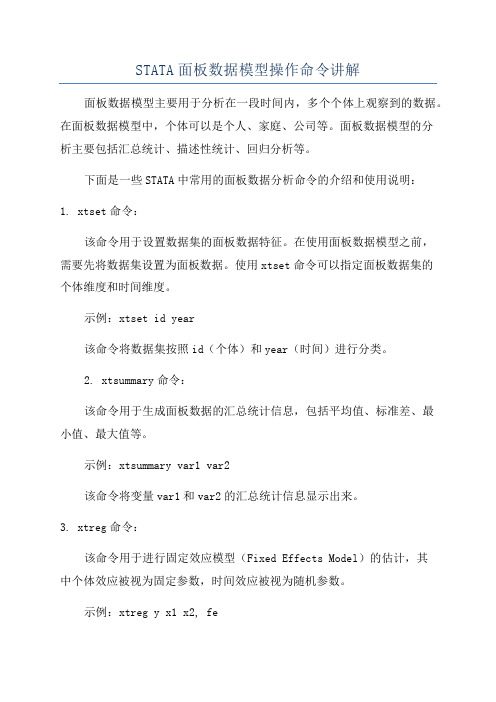
STATA面板数据模型操作命令讲解面板数据模型主要用于分析在一段时间内,多个个体上观察到的数据。
在面板数据模型中,个体可以是个人、家庭、公司等。
面板数据模型的分析主要包括汇总统计、描述性统计、回归分析等。
下面是一些STATA中常用的面板数据分析命令的介绍和使用说明:1. xtset命令:该命令用于设置数据集的面板数据特征。
在使用面板数据模型之前,需要先将数据集设置为面板数据。
使用xtset命令可以指定面板数据集的个体维度和时间维度。
示例:xtset id year该命令将数据集按照id(个体)和year(时间)进行分类。
2. xtsummary命令:该命令用于生成面板数据的汇总统计信息,包括平均值、标准差、最小值、最大值等。
示例:xtsummary var1 var2该命令将变量var1和var2的汇总统计信息显示出来。
3. xtreg命令:该命令用于进行固定效应模型(Fixed Effects Model)的估计,其中个体效应被视为固定参数,时间效应被视为随机参数。
示例:xtreg y x1 x2, fe该命令将变量y对x1和x2进行固定效应模型估计。
4. xtfe命令:该命令用于进行固定效应模型的估计,并提供了更多的选项和功能。
示例:xtfe y x1 x2, vce(robust)该命令将变量y对x1和x2进行固定效应模型估计,并使用鲁棒标准误。
5. xtlogit命令:该命令用于进行面板Logistic回归分析,适用于因变量为二分类变量的情况。
示例:xtlogit y x1 x2, re该命令将变量y对x1和x2进行面板Logistic回归分析,并进行随机效应的估计。
6. areg命令:该命令用于进行差别法(Difference-in-Differences)模型的估计,适用于时间和个体差异的面板数据分析。
上述命令只是STATA中一部分常用的面板数据模型操作命令。
在实际应用中,根据具体的研究需求和数据特征,还可以使用其他面板数据模型命令进行分析,如xtlogit、xtprobit等。
stata命令大全(全)
********* 面板数据计量分析与软件实现 *********说明:以下do文件相当一部分内容来自于中山大学连玉君STATA教程,感谢他的贡献。
本人做了一定的修改与筛选。
*----------面板数据模型* 1.静态面板模型:FE 和RE* 2.模型选择:FE vs POLS, RE vs POLS, FE vs RE (pols混合最小二乘估计) * 3.异方差、序列相关和截面相关检验* 4.动态面板模型(DID-GMM,SYS-GMM)* 5.面板随机前沿模型* 6.面板协整分析(FMOLS,DOLS)*** 说明:1-5均用STATA软件实现, 6用GAUSS软件实现。
* 生产效率分析(尤其指TFP):数据包络分析(DEA)与随机前沿分析(SFA)*** 说明:DEA由DEAP2.1软件实现,SFA由Frontier4.1实现,尤其后者,侧重于比较C-D与Translog生产函数,一步法与两步法的区别。
常应用于地区经济差异、FDI 溢出效应(Spillovers Effect)、工业行业效率状况等。
* 空间计量分析:SLM模型与SEM模型*说明:STATA与Matlab结合使用。
常应用于空间溢出效应(R&D)、财政分权、地方政府公共行为等。
* ---------------------------------* --------一、常用的数据处理与作图-----------* ---------------------------------* 指定面板格式xtset id year (id为截面名称,year为时间名称)xtdes /*数据特征*/xtsum logy h /*数据统计特征*/sum logy h /*数据统计特征*/*添加标签或更改变量名label var h "人力资本"rename h hum*排序sort id year /*是以STATA面板数据格式出现*/sort year id /*是以DEA格式出现*/*删除个别年份或省份drop if year<1992drop if id==2 /*注意用==*/*如何得到连续year或id编号(当完成上述操作时,year或id就不连续,为形成panel 格式,需要用egen命令)egen year_new=group(year)xtset id year_new**保留变量或保留观测值keep inv /*删除变量*/**或keep if year==2000**排序sort id year /*是以STATA面板数据格式出现sort year id /*是以DEA格式出现**长数据和宽数据的转换*长>>>宽数据reshape wide logy,i(id) j(year)*宽>>>长数据reshape logy,i(id) j(year)**追加数据(用于面板数据和时间序列)xtset id year*或者xtdestsappend,add(5) /表示在每个省份再追加5年,用于面板数据/tsset*或者tsdes.tsappend,add(8) /表示追加8年,用于时间序列/*方差分解,比如三个变量Y,X,Z都是面板格式的数据,且满足Y=X+Z,求方差var(Y),协方差Cov(X,Y)和Cov(Z,Y)bysort year:corr Y X Z,cov**生产虚拟变量*生成年份虚拟变量tab year,gen(yr)*生成省份虚拟变量tab id,gen(dum)**生成滞后项和差分项xtset id yeargen ylag=l.y /*产生一阶滞后项),同样可产生二阶滞后项*/gen ylag2=L2.ygen dy=D.y /*产生差分项*/*求出各省2000年以前的open inv的平均增长率collapse (mean) open inv if year<2000,by(id)变量排序,当变量太多,按规律排列。
- 1、下载文档前请自行甄别文档内容的完整性,平台不提供额外的编辑、内容补充、找答案等附加服务。
- 2、"仅部分预览"的文档,不可在线预览部分如存在完整性等问题,可反馈申请退款(可完整预览的文档不适用该条件!)。
- 3、如文档侵犯您的权益,请联系客服反馈,我们会尽快为您处理(人工客服工作时间:9:00-18:30)。
xiSubject Table of ContentsThis is the complete contents for all of the Reference manuals.Getting Started[GS]Getting Started manual..................Getting Started with Stata for Macintosh [GS]Getting Started manual......................Getting Started with Stata for Unix [GS]Getting Started manual...................Getting Started with Stata for Windows [U]User’s Guide,Chapter2...................Resources for learning and using Stata [R]help...................................................Obtain online help Data manipulation and managementBasic data commands[R]describe........................Describe contents of data in memory or on disk [R]display.......................................Substitute for a hand calculator [R]drop......................................Eliminate variables or observations [R]edit......................................Edit and list data using Data Editor [R]egen................................................Extensions to generate [R]generate.................................Create or change contents of variable [R]list................................................List values of variables [R]memory.........................................Memory size considerations [R]obs............................Increase the number of observations in a dataset [R]sort............................................................Sort data Functions and expressions[U]User’s Guide,Chapter16............................Functions and expressions [R]egen................................................Extensions to generate [R]functions.......................................................Functions Dates[U]User’s Guide,Section15.5.3....................................Date formats [U]User’s Guide,mands for dealing with dates [R]functions.......................................................Functions Inputting and saving data[U]User’s Guide,mands to input data [R]edit......................................Edit and list data using Data Editor [R]infile...............................Quick reference for reading data into Stata [R]insheet.........................Read ASCII(text)data created by a spreadsheet [R]infile(free format)..........................Read unformatted ASCII(text)data [R]infix(fixed format).......................Read ASCII(text)data infixed format [R]infile(fixed format).........Read ASCII(text)data infixed format with a dictionary [R]input.............................................Enter data from keyboard [R]odbc..........................................Load data from ODBC sources [R]outfile............................................Write ASCII-format dataset [R]outsheet......................................Write spreadsheet-style dataset [R]save.................................................Save and use datasetsxii[R]e shipped dataset [R]e dataset from web Combining data[U]User’s Guide,mands for combining data [R]append...................................................Append datasets [R]merge.....................................................Merge datasets [R]joinby............................Form all pairwise combinations within groups Reshaping datasets[R]collapse.................................Make dataset of means,medians,etc.[R]contract........................................Make dataset of frequencies [R]press data in memory [R]cross..........................Form every pairwise combination of two datasets [R]expand..............................................Duplicate observations [R]fillin................................................Rectangularize dataset [R]obs.............................Increase the number of observations in dataset [R]reshape..........................Convert data from wide to long and vice versa [R]separate...........................................Create separate variables [R]stack..........................................................Stack data [R]statsby.........................Collect statistics for a command across a by list [R]xpose..................................Interchange observations and variables Labeling,display formats,and notes[U]User’s Guide,Section15.5............Formats:controlling how data are displayed [U]User’s Guide,Section15.6....................Dataset,variable,and value labels [R]format.......................................Specify variable display format [R]bel manipulation [R]bel utilities [R]notes..................................................Place notes in data Changing and renaming variables[U]User’s Guide,mands for dealing with categorical variables [R]destring...................................Change string variables to numeric [R]encode..............................Encode string into numeric and vice versa [R]generate.................................Create or change contents of variable [R]mvencode.................Change missing to coded missing value and vice versa [R]order...........................................Reorder variables in dataset [R]recode..........................................Recode categorical variable [R]rename...................................................Rename variable [R]split.........................................Split string variables into parts Examining data[R]pare two datasets [R]codebook....................Produce a codebook describing the contents of data [R]pare two variables [R]count.........................Count observations satisfying specified condition [R]duplicates.............................Detect and delete duplicate observations [R]gsort.........................................Ascending and descending sort [R]inspect........................Display simple summary of data’s characteristicsxiii [R]isid.............................................Check for unique identifiers [R]pctile...................................Create variable containing percentiles [ST]stdes............................................Describe survival-time data [R]summarize..............................................Summary statistics [SVY]svytab..............................................Tables for survey data [R]table...........................................Tables of summary statistics [P]tabdisp.....................................................Display tables [R]tabstat....................................Display table of summary statistics [R]tabsum..........................One-and two-way tables of summary statistics [R]tabulate...............................One-and two-way tables of frequencies [XT]xtdes...........................................Describe pattern of xt data Miscellaneous data commands[R]corr2data...................Create a dataset with a specified correlation structure [R]drawnorm............................Draw a sample from a normal distribution [R]icd9...............................ICD-9-CM diagnostic and procedures codes [R]ipolate................................Linearly interpolate(extrapolate)values [R]range..............................Numerical ranges,derivatives,and integrals [R]sample...............................................Draw random sample UtilitiesBasic utilities[U]User’s Guide,Chapter8..................Stata’s online help and search facilities [U]User’s Guide,Chapter18.........................Printing and preserving output [U]User’s Guide,Chapter19...........................................Do-files [R]about...........................Display information about my version of Stata [R]by...............................Repeat Stata command on subsets of the data [R]copyright......................................Display copyright information [R]do...........................................Execute commands from afile [R]doedit.......................................Edit do-files and other textfiles [R]exit............................................................Exit Stata [R]help...................................................Obtain online help [R]level............................................Set default confidence level [R]log....................................Echo copy of session tofile or device [R]obs.............................Increase the number of observations in dataset [R]#review.........................................Review previous commands [R]search...........................................Search Stata documentation [R]translate.............................................Print and translate logs [R]view...................................................Viewfiles and logs Error messages[U]User’s Guide,Chapter11.......................Error messages and return codes [R]error messages................................Error messages and return codes [P]error..................................Display generic error message and exit [P]rmsg.....................................................Return messages Saved results[U]User’s Guide,Section16.6................Accessing results from Stata commands [U]User’s Guide,Section21.8..........Accessing results calculated by other programsxiv[U]User’s Guide,Section21.9....Accessing results calculated by estimation commands [U]User’s Guide,Section21.10....................................Saving results [P]creturn...............................................Return c-class values [R]estimates.........................................Manage estimation results [P]return.................................................Return saved results [R]saved results.................................................Saved results Internet[U]User’s Guide,ing the Internet to keep up to date [R]checksum.........................................Calculate checksum offile [R]net.......................Install and manage user-written additions from the net [R]net search.............................Search Internet for installable packages [R]mands to control Internet connections [R]news....................................................Report Stata news [R]sj...............................Stata Journal and STB installation instructions [R]ssc...................................Install and uninstall packages from SSC [R]update......................................................Update Stata Data types and memory[U]User’s Guide,Chapter7............................Setting the size of memory [U]User’s Guide,Section15.2.2............................Numeric storage types [U]User’s Guide,Section15.4.4..............................String storage types [U]User’s Guide,Section16.10......................Precision and problems therein [U]User’s Guide,mands for dealing with strings [R]press data in memory [R]data types....................................Quick reference for data types [R]limits............................................Quick reference for limits [R]matsize.......................Set the maximum number of variables in a model [R]memory.........................................Memory size considerations [R]missing values..............................Quick reference for missing values [R]recast.......................................Change storage type of variable Advanced utilities[R]assert.................................................Verify truth of claim [R]cd.......................................................Change directory [R]checksum.........................................Calculate checksum offile [R]copy............................................Copyfile from disk or URL [R]unch dialog [P]dialogs................................................Dialog programming [R]dir.....................................................Displayfilenames [P]discard...................................Drop automatically loaded programs [R]erase.....................................................Erase a diskfile [P]hexdump..................................Display hexadecimal report onfile [R]mkdir....................................................Create directory [R]more...............................................The—more—message [R]query............................................Display system parameters [P]quietly............................Quietly and noisily perform Stata command [R]set....................................Quick reference for system parameters [R]shell....................................Temporarily invoke operating system [P]smcl......................................Stata markup and control language [P]sysdir................................................Set system directoriesxv [R]type...............................................Display contents offiles [R]which.............................Display location and version for an ado-fileGraphics[G]Graphics manual.............................Stata Graphics Reference Manual[R]boxcox.........................................Box–Cox regression models [TS]corrgram....................................................Correlogram [TS]cumsp......................................Cumulative spectral distribution [R]cumul..............................................Cumulative distribution [R]cusum..............................Cusum plots and tests for binary variables [R]diagnostic plots.................................Distributional diagnostic plots [R]parative scatterplots [R]factor.....................................................Factor analysis [R]grmeanby.....................Graph means and medians by categorical variables [R]histogram....................Histograms for continuous and categorical variables [R]kdensity..................................Univariate kernel density estimation [R]lowess.................................................Lowess smoothing [ST]ltable...........................................Life tables for survival data [R]lv....................................................Letter-value displays [R]mkspline.........................................Linear spline construction [R]pca............................................Principal component analysis [TS]pergram.....................................................Periodogram [R]qc...................................................Quality control charts [R]regression diagnostics..................................Regression diagnostics [R]roc............................Receiver-Operating-Characteristic(ROC)analysis [R]serrbar.......................................Graph standard error bar chart [R]smooth..........................................Robust nonlinear smoother [R]spikeplot........................................Spike plots and rootograms [ST]stphplot.........Graphical assessment of the Cox proportional hazards assumption [ST]streg............Graph estimated survivor,hazard,and cumulative hazard functions [ST]sts graph.............Graph the survivor,hazard,and cumulative hazard functions [R]stem................................................Stem-and-leaf displays [TS]wntestb.......................Bartlett’s periodogram-based test for white noise [TS]xcorr..............................Cross-correlogram for bivariate time series StatisticsBasic statistics[R]egen................................................Extensions to generate [R]anova....................................Analysis of variance and covariance [R]bitest.............................................Binomial probability test [R]ci......................Confidence intervals for means,proportions,and counts [R]correlate.....................Correlations(covariances)of variables or estimators [R]logistic.................................................Logistic regression [R]oneway........................................One-way analysis of variance [R]prtest...............................One-and two-sample tests of proportionsxvi[R]regress..................................................Linear regression [R]predict..................Obtain predictions,residuals,etc.after estimation[R]predictnl...Obtain nonlinear predictions,standard errors,etc.after estimation[R]regression diagnostics............................Regression diagnostics[R]test..............................Test linear hypotheses after estimation[R]testnl.........................Test nonlinear hypotheses after estimation [R]sampsi..................................Sample size and power determination [R]sdtest............................................Variance comparison tests [R]signrank........................................Sign,rank,and median tests [R]statsby.........................Collect statistics for a command across a by list [R]summarize..............................................Summary statistics [R]table...........................................Tables of summary statistics [R]tabstat....................................Display table of summary statistics [R]tabsum..........................One-and two-way tables of summary statistics [R]tabulate...............................One-and two-way tables of frequencies [R]ttest................................................Mean comparison tests ANOV A and related[U]User’s Guide,Chapter29................Overview of Stata estimation commands [R]anova....................................Analysis of variance and covariance [R]rge one-way ANOV A,random effects,and reliability [R]manova........................Multivariate analysis of variance and covariance [R]oneway........................................One-way analysis of variance [R]pkcross.......................................Analyze crossover experiments [R]pkshape..........................Reshape(pharmacokinetic)Latin square data Linear regression and related maximum-likelihood regressions[U]User’s Guide,Chapter29................Overview of Stata estimation commands [U]User’s Guide,Chapter23...............Estimation and post-estimation commands [U]User’s Guide,Section23.14..................Obtaining robust variance estimates [R]estimation commands..................Quick reference for estimation commands [R]areg.........................Linear regression with a large dummy-variable set [R]cnsreg..........................................Constrained linear regression [R]eivreg..........................................Errors-in-variables regression [R]fracpoly.....................................Fractional polynomial regression [R]frontier...........................................Stochastic frontier models [R]glm..............................................Generalized linear models [R]heckman.........................................Heckman selection model [R]impute.......................................Impute data for missing values [R]ivreg................Instrumental variables and two-stage least squares regression [R]mfp...............................Multivariable fractional polynomial models [R]mvreg...............................................Multivariate regression [R]nbreg..........................................Negative binomial regression [TS]newey............................Regression with Newey–West standard errors [R]nl.................................................Nonlinear least squares [R]orthog........................Orthogonal variables and orthogonal polynomials [R]poisson.................................................Poisson regression [TS]prais..................Prais–Winsten regression and Cochrane–Orcutt regression [R]qreg...................................Quantile(including median)regression [R]reg3................Three-stage estimation for systems of simultaneous equationsxvii [R]regress..................................................Linear regression [R]regression diagnostics..................................Regression diagnostics [R]roc............................Receiver-Operating-Characteristic(ROC)analysis [R]rreg.....................................................Robust regression [ST]stcox....................................Fit Cox proportional hazards model [ST]streg.........................................Fit parametric survival models [R]sureg................................Zellner’s seemingly unrelated regression [SVY]svy estimators....................Estimation commands for complex survey data [R]sw..................................Stepwise maximum-likelihood estimation [R]tobit............................Tobit,censored-normal,and interval regression [R]treatreg.............................................Treatment effects model [R]truncreg...............................................Truncated regression [R]vwls........................................Variance-weighted least squares [XT]xtabond....................Arellano–Bond linear,dynamic panel-data estimator [XT]xtfrontier.............................Stochastic frontier models for panel data [XT]xtgee......................Fit population-averaged panel-data models using GEE [XT]xtgls........................................Fit panel-data models using GLS [XT]xtintreg..........................Random-effects interval data regression models [XT]xthtaylor................Hausman–Taylor estimator for error components models [XT]xtivreg.....Instrumental variables and two-stage least squares for panel-data models [XT]xtnbreg Fixed-effects,random-effects,and population-averaged negative binomial models [XT]xtpcse...........OLS or Prais–Winsten models with panel-corrected standard errors [XT]xtpoisson....Fixed-effects,random-effects,and population-averaged Poisson models [XT]xtrchh.............................Hildreth–Houck random coefficients models [XT]xtreg...Fixed-,between-,and random-effects and population-averaged linear models [XT]xtregar.........Fixed-and random-effects linear models with an AR(1)disturbance [R]zip.........................Zero-inflated Poisson and negative binomial models Logistic and probit regression[U]User’s Guide,Chapter29................Overview of Stata estimation commands [U]User’s Guide,Chapter23...............Estimation and post-estimation commands [U]User’s Guide,Section23.14..................Obtaining robust variance estimates [R]biprobit............................................Bivariate probit models [R]clogit.............................Conditional(fixed-effects)logistic regression [R]cloglog...................Maximum-likelihood complementary log-log estimation [R]constraint.........................................Define and list constraints [R]glogit......................................Logit and probit on grouped data [R]heckprob...................Maximum-likelihood probit estimation with selection [R]hetprob....................Maximum-likelihood heteroskedastic probit estimation [R]logistic.................................................Logistic regression [R]logit....................................Maximum-likelihood logit estimation [R]mlogit..........Maximum-likelihood multinomial(polytomous)logistic regression [R]nlogit.............................Maximum-likelihood nested logit estimation [R]ologit............................Maximum-likelihood ordered logit estimation [R]oprobit..........................Maximum-likelihood ordered probit estimation [R]probit..................................Maximum-likelihood probit estimation [R]rologit......................................Rank-ordered logistic regression [R]scobit............................Maximum-likelihood skewed logit estimation [SVY]svy estimators....................Estimation commands for complex survey data [R]sw..................................Stepwise maximum-likelihood estimation [XT]xtcloglog................Random-effects and population-averaged cloglog modelsxviii[XT]xtgee......................Fit population-averaged panel-data models using GEE [XT]xtlogit.........Fixed-effects,random-effects,and population-averaged logit models [XT]xtprobit..................Random-effects and population-averaged probit models Pharmacokinetic statistics[U]User’s Guide,Section29.18..............................Pharmacokinetic data [R]pk..................................Pharmacokinetic(biopharmaceutical)data [R]pkcollapse.......................Generate pharmacokinetic measurement dataset [R]pkcross.......................................Analyze crossover experiments [R]pkexamine................................Calculate pharmacokinetic measures [R]pkequiv........................................Perform bioequivalence tests [R]pkshape..........................Reshape(pharmacokinetic)Latin square data [R]pksumm....................................Summarize pharmacokinetic data Survival analysis[U]User’s Guide,Chapter29................Overview of Stata estimation commands [U]User’s Guide,Chapter23...............Estimation and post-estimation commands [U]User’s Guide,Section23.14..................Obtaining robust variance estimates [ST]ct.......................................................Count-time data [ST]ctset......................................Declare data to be count-time data [ST]cttost............................Convert count-time data to survival-time data [ST]ltable...........................................Life tables for survival data [ST]snapspan.............................Convert snapshot data to time-span data [ST]st......................................................Survival-time data [ST]st is............................Survival analysis subroutines for programmers [ST]stbase................................................Form baseline dataset [ST]stci...............Confidence intervals for means and percentiles of survival time [ST]stcox....................................Fit Cox proportional hazards model [ST]stdes............................................Describe survival-time data [ST]stfill...........................Fill in by carrying forward values of covariates [ST]stgen.............................Generate variables reflecting entire histories [ST]stir........................................Report incidence-rate comparison [ST]stphplot.........Graphical assessment of the Cox proportional hazards assumption [ST]stptime.........................Calculate person-time,incidence rates,and SMR [ST]strate....................................Tabulate failure rates and rate ratios [ST]streg.........................................Fit parametric survival models [ST]sts......Generate,graph,list,and test the survivor and cumulative hazard functions [ST]sts generate.........................Create survivor,hazard,and other variables [ST]sts graph.................Graph the survivor and the cumulative hazard functions [ST]sts list....................List the survivor and the cumulative hazard functions [ST]sts test....................................Test equality of survivor functions [ST]stset....................................Declare data to be survival-time data [ST]stsplit.......................................Split and join time-span records [ST]stsum.........................................Summarize survival-time data [ST]sttocc..........................Convert survival-time data to case–control data [ST]sttoct............................Convert survival-time data to count-time data [ST]stvary..................................Report which variables vary over time [R]sw..................................Stepwise maximum-likelihood estimationxixTime series[U]User’s Guide,Section14.4.3...............................Time-series varlists [U]User’s Guide,Section15.5.4..............................Time-series formats [U]User’s Guide,Section16.8...............................Time-series operators [U]User’s Guide,Section27.3..................................Time-series dates [U]User’s Guide,Section29.12........................Models with time-series data [TS]time series...............................Introduction to time-series commands [TS]arch......Autoregressive conditional heteroskedasticity(ARCH)family of estimators [TS]arima.........................Autoregressive integrated moving average models [TS]corrgram....................................................Correlogram [TS]cumsp......................................Cumulative spectral distribution [TS]dfgls..........................................Perform DF-GLS unit-root test [TS]dfuller...........................Augmented Dickey–Fuller test for a unit root [TS]newey............................Regression with Newey–West standard errors [TS]pergram.....................................................Periodogram [TS]pperron....................................Phillips–Perron test for unit roots [TS]prais..................Prais–Winsten regression and Cochrane–Orcutt regression [TS]regression diagnostics.....................Regression diagnostics for time series [TS]tsappend...............................Add observations to time-series dataset [TS]tsreport.................Report time-series aspects of dataset or estimation sample [TS]tsrevar............................Time-series operator programming command [TS]tsset....................................Declare dataset to be time-series data [TS]tssmooth.......................Smooth and forecast univariate time-series data [TS]tssmooth dexponential..........................Double exponential smoothing [TS]tssmooth exponential..................................Exponential smoothing [TS]tssmooth hwinters.........................Holt–Winters nonseasonal smoothing [TS]tssmooth ma..........................................Moving-averagefilter [TS]tssmooth nl................................................Nonlinearfilter [TS]tssmooth shwinters...........................Holt–Winters seasonal smoothing [TS]var intro........................An introduction to vector autoregression models [TS]var...........................................Vector autoregression models [TS]var svar...............................Structural vector autoregression models [TS]varbasic..................Fit a simple V AR and graph impulse response functions [TS]varfcast pute dynamic forecasts of dependent variables after var or svar [TS]varfcast graph............Graph forecasts of dependent variables after var or svar [TS]vargranger..............Perform pairwise Granger causality tests after var or svar [TS]varirf.................................An introduction to the varirf commands [TS]varirf add...................Add V ARIRF results from one V ARIRFfile to another [TS]varirf cgraph......Make combined graphs of impulse response functions and FEVD s [TS]varirf create....Obtain impulse response functions and forecast error decompositions [TS]varirf ctable.......Make combined tables of impulse response functions and FEVD s [TS]varirf describe........................................Describe a V ARIRFfile [TS]varirf dir..................................List the V ARIRFfiles in a directory [TS]varirf drop......................Drop V ARIRF results from the active V ARIRFfile [TS]varirf erase.............................................Erase a V ARIRFfile [TS]varirf graph.......................Graph impulse response functions and FEVD s [TS]varirf ograph...............Graph overlaid impulse response functions and FEVD s [TS]varirf rename..........................Rename a V ARIRF result in a V ARIRFfile [TS]varirf set.............................................Set active V ARIRFfile [TS]varirf table................Create tables of impulse response functions and FEVD s [TS]varlmar...........Obtain LM statistics for residual autocorrelation after var or svar。