The effect of turbulent intermittency on the deflagration to detonation transition in SN Ia
The effect of climate on acoustic signals中文翻译

气候变化对声学信号的影响:大气吸声是否会对鸟的歌声和蝙蝠的定位叫声造成影响?生态学和进化生物学系,图森,亚利桑那大学,1041东洛厄尔街,亚利桑那州85721 沿着生态梯度的信号差异可能会导致新物种生成。
目前的研究验证了这个假说,沿气候梯度的声音吸收的变化为声学信号的差异做出了选择,这不仅有助于理解物种的多样性,而且对了解生物如何应对气候变化也有帮助。
由于吸声会随温度、湿度和声音频率而变化,个体或物种的信号结构可能会随空间或时间上的气候变化而改变。
特别是具有较低频率、较窄带宽和较长持续时间的信号在高吸声环境中应该会更易检测到。
通过研究北美木莺和美国西南地区的蝙蝠,这项工作发现了信号结构和吸声之间存在关联的证据。
整个活动范围具有较高的平均吸收值的莺鸟更可能具有较窄带宽的歌声。
在具有较高吸收值的栖息地发现的蝙蝠种类更可能有较低频率的叫声。
此外,蝙蝠的定位叫声结构会随着季节而变化。
在具有较高吸声的雨季中,蝙蝠会使用具有较长持续时间、较低频率的叫声。
这些结果表明,尽管吸声的影响不算太大,但由于吸声的变化,信号可能会随着气候梯度发生改变。
1 绪论因为环境会影响声学和视觉信号从信号发送者到接收者的传输方式(Morton, 1975; Wiley 和Richards, 1978; Richards 和Wiley, 1980; Endler,2000),所以信号系统往往会沿生态梯度发生改变(Hunter 和Krebs,1979; Wiley, 1991; Marchetti,1993;Badyaev和Leaf,1997;McNaught and Owens, 2002;Slabbekoorn and Smith, 2002; Tobias et al., 2010)。
这种改变对于物种的形成和多样化有重要意义,因为信号方面的变化可能导致合子前隔离(West-Eberhard, 1983; Endler, 1992;Schluter 和Price, 1993; Grant 和Grant, 1996; Irwin 等,2001)。
Jet Impingement Heat Transfer Ch06-P020039
Jet Impingement Heat Transfer: Physics,Correlations,and Numerical ModelingN.ZUCKERMAN and N.LIORDepartment of Mechanical Engineering and Applied Mechanics,The University of Pennsylvania, Philadelphia,PA,USA;E-mail:zuckermn@;lior@I.SummaryThe applications,physics of theflow and heat transfer phenomena, available empirical correlations and values they predict,and numerical simulation techniques and results of impinging jet devices for heat transfer are described.The relative strengths and drawbacks of the k–e,k–o, Reynolds stress model,algebraic stress models,shear stress transport,and v2f turbulence models for impinging jetflow and heat transfer are compared. Select model equations are provided as well as quantitative assessments of model errors and judgments of model suitability.II.IntroductionWe seek to understand theflowfield and mechanisms of impinging jets with the goal of identifying preferred methods of predicting jet performance. Impinging jets provide an effective andflexible way to transfer energy or mass in industrial applications.A directed liquid or gaseousflow released against a surface can efficiently transfer large amounts of thermal energy or mass between the surface and thefluid.Heat transfer applications include cooling of stock material during material forming processes,heat treatment [1],cooling of electronic components,heating of optical surfaces for defogging,cooling of turbine components,cooling of critical machinery structures,and many other industrial processes.Typical mass transfer applications include drying and removal of small surface particulates. Abrasion and heat transfer by impingement are also studied as side effects of vertical/short take-off and landing jet devices,for example in the case of direct lift propulsion systems in vertical/short take-off and landing aircraft.Advances in Heat TransferVolume39ISSN0065-2717DOI:10.1016/S0065-2717(06)39006-5565Copyright r2006Elsevier Inc.All rights reservedADVANCES IN HEAT TRANSFER VOL.39566N.ZUCKERMAN AND N.LIORGeneral uses and performance of impinging jets have been discussed in a number of reviews[2–5].In the example of turbine cooling applications[6],impinging jetflows may be used to cool several different sections of the engine such as the combustor case(combustor can walls),turbine case/liner,and the critical high-temperature turbine blades.The gas turbine compressor offers a steadyflow of pressurized air at temperatures lower than those of the turbine and of the hot gasesflowing around it.The blades are cooled using pressurized bleed flow,typically available at6001C.The bleed air must cool a turbine immersed in gas of14001C total temperature[7],which requires transfer coefficients in the range of1000–3000W/m2K.This equates to a heatflux on the order of 1MW/m2.The ability to cool these components in high-temperature regions allows higher cycle temperature ratios and higher efficiency,improving fuel economy,and raising turbine power output per unit weight.Modern turbines have gas temperatures in the main turbineflow in excess of the temperature limits of the materials used for the blades,meaning that the structural strength and component life are dependent upon effective coolingflow. Compressor bleedflow is commonly used to cool the turbine blades by routing it through internal passages to keep the blades at an acceptably low temperature.The same air can be routed to a perforated internal wall to form impinging jets directed at the blade exterior wall.Upon exiting the blade,the air may combine with the turbine core airflow.Variations on this design may combine the impinging jet device with internalfins,smooth or roughened cooling passages,and effusion holes forfilm cooling.The designer may alter the spacing or locations of jet and effusion holes to concentrate theflow in the regions requiring the greatest cooling.Though the use of bleed air carries a performance penalty[8],the small amount offlow extracted has a small influence on bleed air supply pressure and temperature.In addition to high-pressure compressor air,turbofan engines provide cooler fan air at lower pressure ratios,which can be routed directly to passages within the turbine liner.A successful design uses the bleed air in an efficient fashion to minimize the bleedflow required for maintaining a necessary cooling rate. Compared to other heat or mass transfer arrangements that do not employ phase change,the jet impingement device offers efficient use of the fluid,and high transfer rates.For example,compared with conventional convection cooling by confinedflow parallel to(under)the cooled surface, jet impingement produces heat transfer coefficients that are up to three times higher at a given maximumflow speed,because the impingement boundary layers are much thinner,and often the spentflow after the impingement serves to turbulate the surroundingfluid.Given a required heat transfer coefficient,theflow required from an impinging jet device may be two orders of magnitude smaller than that required for a cooling approach usinga free wall-parallel flow.For more uniform coverage over larger surfaces multiple jets may be used.The impingement cooling approach also offers a compact hardware arrangement.Some disadvantages of impingement cooling devices are:(1)For moving targets with very uneven surfaces,the jet nozzles may have to be located too far from the surface.For jets starting at a large height above the target (over 20jet nozzle diameters)the decay in kinetic energy of the jet as it travels to the surface may reduce average Nu by 20%or more.(2)The hardware changes necessary for implementing an impinging jet device may degrade structural strength (one reason why impinging jet cooling is more easily applied to turbine stator blades than to rotor blades).(3)In static applications where very uniform surface heat or mass transfer is required,the resulting high density of the jet array and corresponding small jet height may be impractical to construct and implement,and at small spacings jet-to-jet interaction may degrade efficiency.Prior to the design of an impinging jet device,the heat transfer at the target surface is typically characterized by a Nusselt number (Nu ),and the mass transfer from the surface with a Schmidt number (Sc ).For design efficiency studies and device performance assessment,these values are tracked vs.jet flow per unit area (G )or vs.the power required to supply the flow (incremental compressor power).A.I MPINGING J ET R EGIONSThe flow of a submerged impinging jet passes through several distinct regions,as shown in Fig.1.The jet emerges from a nozzle or opening with a velocity and temperature profile and turbulence characteristics dependent upon the upstream flow.For a pipe-shaped nozzle,also called a tube nozzle or cylindrical nozzle,the flow develops into the parabolic velocity profile common to pipe flow plus a moderate amount of turbulence developed upstream.In contrast,a flow delivered by application of differential pressure across a thin,flat orifice will create an initial flow with a fairly flat velocity profile,less turbulence,and a downstream flow contraction (vena contracta).Typical jet nozzles designs use either a round jet with an axisymmetric flow profile or a slot jet ,a long,thin jet with a two-dimensional flow profile.After it exits the nozzle,the emerging jet may pass through a region where it is sufficiently far from the impingement surface to behave as a free submerged jet.Here,the velocity gradients in the jet create a shearing at the edges of the jet which transfers momentum laterally outward,pulling additional fluid along with the jet and raising the jet mass flow,as shown in Fig.2.In the process,the jet loses energy and the velocity profile is widened in spatial extent and decreased in magnitude along the sides of the jet.Flow interior to the 567JET IMPINGEMENT HEAT TRANSFERprogressively widening shearing layer remains unaffected by this momentum transfer and forms a core region with a higher total pressure,though it may experience a drop in velocity and pressure decay resulting from velocity gradients present at the nozzle exit.A free jet region may not exist if the nozzle lies within a distance of two diameters (2D )from the target.In such cases,the nozzle is close enough to the elevated static pressure in the stagnation region for this pressure to influence the flow immediately at the nozzle exit.If the shearing layer expands inward to the center of the jet prior to reaching the target,a region of core decay forms.For purposes of distinct identification,the end of the core region may be defined as the axial position where the centerline flow dynamic pressure (proportional to speed squared)reaches 95%of its original value.This decaying jet begins four to eight nozzle diameters or slot-widths downstream of the nozzle exit.In the decaying jet,the axial velocity component in the central part decreases,with theradialF IG .1.The flow regions of an impinging jet.568N.ZUCKERMAN AND N.LIORvelocity profile resembling a Gaussian curve that becomes wider and shorter with distance from the nozzle outlet.In this region,the axial velocity and jet width vary linearly with axial position.Martin [2]provided a collection of equations for predicting the velocity in the free jet and decaying jet regions based on low Reynolds number flow.Viskanta [5]further subdivided this region into two zones,the initial ‘‘developing zone,’’and the ‘‘fully developed zone’’in which the decaying free jet reaches a Gaussian velocity profile.As the flow approaches the wall,it loses axial velocity and turns.This region is labeled the stagnation region or deceleration region.The flow builds up a higher static pressure on and above the wall,transmitting the effect of the wall upstream.The nonuniform turning flow experiences high normal and shear stresses in the deceleration region,which greatly influence local transport properties.The resulting flow pattern stretches vortices in the flow and increases the turbulence.The stagnation region typically extends1.2nozzle diameters above the wall for round jets [2].Experimental work by Maurel and Solliec [9]found that this impinging zone was characterized or delineated by a negative normal-parallel velocity correlation (uv o 0).For their slot jet this region extended to 13%of the nozzle height H ,and did not vary with Re or H /D.F IG .2.The flow field of a free submerged jet.569JET IMPINGEMENT HEAT TRANSFERAfter turning,theflow enters a wall jet region where theflow moves laterally outward parallel to the wall.The wall jet has a minimum thickness within0.75–3diameters from the jet axis,and then continually thickens moving farther away from the nozzle.This thickness may be evaluated by measuring the height at which wall-parallelflow speed drops to some fraction(e.g.5%)of the maximum speed in the wall jet at that radial position.The boundary layer within the wall jet begins in the stagnation region,where it has a typical thickness of no more than1%of the jet diameter[2].The wall jet has a shearing layer influenced by both the velocity gradient with respect to the stationaryfluid at the wall(no-slip condition) and the velocity gradient with respect to thefluid outside the wall jet.As the wall jet progresses,it entrainsflow and grows in thickness,and its average flow speed decreases as the location of highestflow speed shifts progressively farther from the wall.Due to conservation of momentum,the core of the wall jet may accelerate after theflow turns and as the wall boundary layer develops.For a round jet,mass conservation results in additional deceleration as the jet spreads radially outward.B.N ONDIMENSIONAL H EAT AND M ASS T RANSFER C OEFFICIENTSA major parameter for evaluating heat transfer coefficients is the Nusselt number,Nu¼hD h=k cð1Þwhere h is the convective heat transfer coefficient defined ash¼Àk c@T.@n*T0jetÀT wallð2Þwhere@T/@n gives the temperature gradient component normal to the wall. The selection of Nusselt number to measure the heat transfer describes the physics in terms offluid properties,making it independent of the target characteristics.The jet temperature used,T0jet,is the adiabatic wall temperature of the decelerated jetflow,a factor of greater importance at increasing Mach numbers.The non-dimensional recovery factor describes how much kinetic energy is transferred into and retained in thermal form as the jet slows down:recovery factor¼T wallÀT0jetU2jet.2c pð3Þ570N.ZUCKERMAN AND N.LIORThis definition may introduce some complications in laboratory work,as a test surface is rarely held at a constant temperature,and more frequently held at a constant heat flux.Experimental work by Goldstein et al .[10]showed that the temperature recovery factor varies from 70%to 110%of the full theoretical recovery,with lowered recoveries in the stagnation region of a low-H /D jet (H /D ¼2),and 100%elevated stagnation region recoveries for jets with H /D ¼6and higher.The recovery comes closest to uniformity for intermediate spacings around H /D ¼5.Entrainment of surrounding flow into the jet may also influence jet performance,changing the fluid temperature as it approaches the target.The nondimensional Sherwood number defines the rate of mass transfer in a similar fashion:Sh ¼k i D =D ið4Þk i ¼D i @C =@n ÂÃ=C 0jet ÀC wall ÂÃð5Þwhere @C /@n gives the mass concentration gradient component normal to the wall.With sufficiently low mass concentration of the species of interest,the spatial distribution of concentration will form patterns similar to those of the temperature pattern.Studies of impinging air jets frequently use the nondimensional relation:Nu =Sh ¼Pr =Sc ÀÁ0:4ð6Þto relate heat and mass transfer rates.The nondimensional parameters selected to describe the impinging jet heat transfer problem include the fluid properties such as Prandtl number Pr (the ratio of fluid thermal diffusivity to viscosity,fairly constant),plus the following:H /D :nozzle height to nozzle diameter ratio; r /D :nondimensional radial position from the center of the jet; z /D :nondimensional vertical position measured from the wall;Tu :nondimensional turbulence intensity,usually evaluated at the nozzle; Re 0:Reynolds number U 0D /n ;M :Mach number (the flow speed divided by speed of sound in the fluid),based on nozzle exit average velocity (of smaller importance at low speeds,i.e.M o 0.3);p jet /D :jet center-to-center spacing (pitch)to diameter ratio,for multiple jets;571JET IMPINGEMENT HEAT TRANSFERAf :free area(¼1À[total nozzle exit area/total target area]);f:relative nozzle area(¼total nozzle exit area/total target area). Thefluid properties are conventionally evaluated using theflow at the nozzle exit as a reference location.Characteristics at the position provide the averageflow speed,fluid temperature,viscosity,and length scale D.In the case of a slot jet the diameter D is replaced in some studies by slot width B, or slot hydraulic diameter2B in others.A complete description of the problem also requires knowledge of the velocity profile at the nozzle exit,or equivalent information about theflow upstream of the nozzle,as well as boundary conditions at the exit of the impingement region.Part of the effort of comparing information about jet impingement is to thoroughly know the nature and magnitude of the turbulence in theflowfield.The geometry andflow conditions for the impinging jet depend upon the nature of the target and thefluid source(compressor or blower).In cases where the pressure drop associated with delivering and exhausting theflow is negligible,the design goal is to extract as much cooling as possible from a given air massflow.Turbine blade passage cooling is an example of such an application;engine compressor air is available at a pressure sufficient to choke theflow at the nozzle(or perhaps at some other point in theflow path).As the bleedflow is a small fraction of the overall compressorflow, the impinging jet nozzle pressure ratio varies very little with changes in the amount of airflow extracted.At high pressure ratios the jet emerges at a high Mach number.In the most extreme case,theflow exits the nozzle as an underexpanded supersonic jet.This jet forms complex interacting shock patterns and a stagnation or recirculation‘‘bubble’’directly below the jet (shown in Fig.3),which may degrade heat transfer[11].The details of the impingement device design affect the system pressuredrop and thus the overall device performance.In the case of adeviceF IG.3.Supersonic jetflow pattern. 572N.ZUCKERMAN AND N.LIORpowered by a blower or compressor,the blower power draw can be predicted using the required pressure rise,flow,and blower efficiency including any losses in the motor or transmission.For incompressible duct flow one can then estimate the power by multiplying the blower pressure rise D p by the volumetric flow Q and then dividing by one or more efficiency factors (e.g.,using a total efficiency of 0.52based on a 0.65blower aerodynamic efficiency times 0.80motor efficiency).This same approach works for calculating pump power when dealing with liquid jets,but becomes more complex when dealing with a turbine-cooling problem where compressibility is significant.The blower pressure rise D p depends on the total of the pressure losses in the blower intake pathway,losses in the flow path leading to the nozzle,any total pressure loss due to jet confinement and jet interaction,and any losses exiting the target region.In cases where space is not critical the intake pathway and nozzle supply pathway are relatively open,for there is no need to accelerate the flow far upstream of the nozzle exit.When possible,the flow is maintained at low speed (relative to U jet )until it nears the nozzle exit,and then accelerated to the required jet velocity by use of a smoothly contracting nozzle at the end of a wide duct or pipe.In such a case,the majority of the loss occurs at the nozzle where the dynamic pressure is greatest.For a cylindrical nozzle,this loss will be at least equal to the nozzle dump loss,giving a minimum power requirement of (0:5r U 2jet Q ).Jet impingement devices have pressure losses from the other portions of the flow path,and part of the task of improving overall device performance is to reduce these other losses.For this reason,one or more long,narrow supply pipes (common in experimental studies)may not make an efficient device due to high frictional losses approaching the nozzle exit.When orifice plate nozzles are used the upstream losses are usually small,but the orifices can cause up to 2.5times the pressure drop of short,smooth pipe nozzles (at a set Q and D ).This effect is balanced against the orifice nozzle’s larger shear layer velocity gradient and more rapid increase in turbulence in the free-jet region [12].Such orifice plates take up a small volume for the hardware,and are relatively easy and inexpensive to make.A thicker orifice plate (thickness from 0.3D to 1.5D )allows the making of orifice holes with tapered or rounded entry pathways,similar to the conical and bellmouth shapes used in contoured nozzles.This compromise comes at the expense of greater hardware volume and complexity,but reduces the losses associated with accelerating the flow as it approaches the orifice and increases the orifice discharge coefficient (effective area).Calculation of nozzle pressure loss may use simple handbook equations for a cylindrical nozzle [13,14],but for an orifice plate the calculations may require more specialized equations and test data (cf.[15,16]).573JET IMPINGEMENT HEAT TRANSFERTable I compares characteristics of the most common nozzle geometries in a qualitative fashion.C.T URBULENCE G ENERATION AND E FFECTSJet behavior is typically categorized and correlated by its Reynolds number Re ¼U 0D /n ,defined using initial average flow speed (U 0),the fluid viscosity (n )and the characteristic length that is the nozzle exit diameter D or twice the slot width,2B (the slot jet hydraulic diameter).At Re o 1000the flow field exhibits laminar flow properties.At Re 43000the flow has fully turbulent features.A transition region occurs with 1000o Re o 3000[5].Turbulence has a large effect on the heat and mass transfer rates.Fully laminar jets are amenable to analytical solution,but such jets provide less heat transfer at a given flow rate than turbulent ones,and therefore much more literature exists for turbulent impinging jets.For example,an isolated round jet at Re ¼2000(transition to turbulence),Pr ¼0.7,H /D ¼6will deliver an average Nu of 19over a circular target spanning six jet diameters,while at Re ¼100,000the average Nu on the same target will reach 212[2].In contrast,laminar jets at close target spacing will give Nu values in the range of 2–20.In general,the exponent b in the relationship Nu p Re b ranges from b ¼0.5for low-speed flows with a low-turbulence wall jet,up to b ¼0.85for high Re flows with a turbulence-dominated wall jet.As an example of the possible extremes,Rahimi et al .[17]measured local Nu values as high as 1700for a under-expanded supersonic jet at Re ¼(1.028)Â106.Typical gas jet installations for heat transfer span a Reynolds number range from 4000to 80,000.H /D typically ranges from 2to 12.Ideally,Nu increases as H decreases,so a designer would prefer to select the smallest tolerable H value,noting the effects of exiting flow,manufacturing TABLE IC OMPARISONOF N OZZLE -T YPE C HARACTERISTICS Nozzle type InitialturbulenceFree jet shearing force Pressure drop Nozzle exit velocity profile Pipe HighLow High Close to parabolic Contoured contraction LowModerate to high Low Uniform (flat)Sharp orificeLow High High Close to uniform(contracting)574N.ZUCKERMAN AND N.LIORcapabilities,and physical constraints,and then select nozzle size D accordingly.For small-scale turbomachinery applications jet arrays commonly have D values of0.2–2mm,while for larger scale industrial applications,jet diameters are commonly in the range of5–30mm. The diameter is heavily influenced by manufacturing and assembly capabilities.Modeling of the turbulentflow,incompressible except for the cases where the Mach number is high,is based on using the well-established mass, momentum,and energy conservation equations based on the velocity, pressure,and temperature:@u i@x i¼0ð7Þr @u i@tþr u i@u j@x j¼À@p@x iþ@s ij@x jþ@t ij@x jð8Þr @u i@tþr u i@u j@x j¼À@p@x iþ@@x jm@u i@x jþ@u j@x i!þ@@x jÀr0ijðalternate formÞð9Þr c p @T@tþr c p u j@T@x j¼s ij@u i@x jþ@@x jm c pPr@T@x jþ@@x jÀr c p u0j T0ÀÁþm@u0i@x jþ@u0j@x i@u0i@x jð10Þs ij¼m@u i@x jþ@u j@x ið11Þt ij¼Àr u0i u0jð12Þwhere an overbar above a single letter represents a time-averaged term, terms with a prime symbol(0)representfluctuating values,and a large overbar represents a correlation.The second moment of the time variant momentum equation,adjusted to extract thefluctuating portion of theflowfield,yields the conserva-tive transport equation for Reynolds stresses,shown for an incompressiblefluid[18]:@t ij @t þ"u k@t ij@x k¼Àt ik@"u j@x kÀt jk@"u i@x k!þp0r@u0i@x jþ@u0j@x i"#þ@@x kÀu0iu0j u0kÀp0ru0id jkþu0j d ikn o!þÀ2n@ui@x k@u0j@x k"#þn@2t ij@x k@x k!ð13ÞEach term of this equation has a specific significance.The term@t ij@t þu k@t ij@x krepresents convective transport of Reynoldsstresses.The termÀt ik@"u j@x k Àt jk@"u i@x kmeasures turbulent production of Reynoldsstresses.The term p0r@ui@x jþ0j@x imeasures the contribution of the pressure-strainrate correlation to Reynolds stresses.The term@@x kÀu0iu0j u0kÀp0ru0id jkþu0j d ikn ogives the effects of thegradient of turbulent diffusion.The termÀ2n@u0i@x kj@x krepresents the effects of turbulent dissipation.The term n@2t ij@x k@x krepresents the effects of molecular diffusion.The specific turbulent kinetic energy k,gives a measure of the intensity of the turbulentflowfield.This can be nondimensionalized by dividing it by the time-averaged kinetic energy of theflow to give the turbulence intensity, based on a velocity ratio:Tu¼ffiffiffiffiffiffiffiffiu0j u0j"u i"u isð14ÞIn addition to generation in the impinging jetflowfield itself,turbulence in theflowfield may also be generated upstream of the nozzle exit and convected into theflow.This often takes place due to the coolantflow distribution configuration,but can also be forced for increasing the heat transfer coefficients,by inserting various screens,tabs,or other obstructions in the jet supply pipe upstream of or at the nozzle.Experimental work has shown that this decreases the length of the jet core region,thus reducing theH/D at which the maximal Nu avg is reached[19].The downstreamflow and heat transfer characteristics are sensitive to both the steady time-averaged nozzle velocity profile andfluctuations in the velocity over time.Knowledge of these turbulentfluctuations and the ability to model them,including associated length scales,are vital for understanding and comparing the behavior and performance of impinging jets.In the initial jet region the primary source of turbulence is the shearflow on the edges of the jet.This shear layer may start as thin as a knife-edge on a sharp nozzle,but naturally grows in area along the axis of the jet.At higher Reynolds numbers,the shear layer generatesflow instability,similar to the Kelvin–Helmholtz instability.Figure4presents in a qualitative fashion the experimentally observed pattern of motion at the edges of the unstable free jet.At highflow speeds(Re41000)the destabilizing effects of shear forces may overcome the stabilizing effect offluid viscosity/momentum diffusion. The position of the shear layer and its velocity profile may develop oscillations in space,seemingly wandering from side to side over time. Further downstream,the magnitude and spatial extent of the oscillations grow to form large-scale eddies along the sides of the jet.The largest eddies have a length scale of the same order of magnitude as the jet diameter and persist until they either independently break up into smaller eddies or meet and interact with other downstreamflow features.The pressurefield of the stagnation region further stretches and distorts the eddies,displacing them laterally until they arrive at the wall.F IG.4.Instability in the turbulent free jet.Experiments by Hoogendorn[20]found that the development of turbulence in the free jet affected the profile of the local Nu on the target stagnation region as well as the magnitude.For pipe nozzles and for contoured nozzles at high spacing(z/D45)the Nu profiles had a peak directly under the jet axis.For contoured nozzles at z/D¼2and4with low initial turbulence(Tu$1%),the maximum Nu occurred in the range0.4o r/D o0.6 with a local minimum at r¼0,typically95%of the peak value.In the decaying jet region the shear layer extends throughout the center of the jet.This shearing promotesflow turbulence,but on smaller scales.The flow in the decaying jet may form small eddies and turbulent pockets within the center of the jet,eventually developing into a unstructured turbulent flowfield with little or no coherent structures in the entire jet core.In the deceleration region,additional mechanisms take part in influencing flowfield turbulence.The pressure gradients within theflowfield cause the flow to turn,influencing the shear layer and turning and stretching large-scale structures.The deceleration of theflow creates normal strains and stresses,which promote turbulence.Numerical models by Abe and Suga[21] showed that the transport of heat or mass in this region is dominated by large-scale eddies,in contrast to the developed wall jet where shear strains dominate.Theflow traveling along the wall may make a transition to turbulence in the fashion of a regular parallel wall jet,beginning with a laminarflow boundary layer region and then reaching turbulence at some lateral position on the wall away from the jet axis.For transitional and turbulent jets,the flow approaching the wall already has substantial turbulence.This turbulent flowfield may contain largefluctuations in the velocity component normal to the wall,a phenomenon distinctly different than those of wall-parallel shearflows[22].Large-scale turbulentflow structures in the free jet have a great effect upon transfer coefficients in the stagnation region and wall jet.The vortices formed in the free jet-shearing layer,categorized as primary vortices,may penetrate into the boundary layer and exchangefluids of differing kinetic energy and temperature(or concentration).The ability of the primary vortex to dynamically scrub away the boundary layer as it travels against and along the wall increases the local heat and mass transfer.The turbulentflowfield along the wall may also cause formation of additional vortices categorized as secondary vortices.Turbulentfluctuations in lateral/radial velocity and associated pressure gradientfluctuations can produce localflow reversals along the wall,initiating separation and the formation of the secondary vortices,as shown in Fig.5.Secondary vortices cause local rises in heat/mass transfer rates and like the primary vortices。
流体力学与传热:Nature of fluids
The distinction between the two types of flow
Laminar flow
Fluid flows without lateral mixing, and there are neither cross-currents and eddies.
Turbulence
Nature of fluids
• Incompressible fluid • Compressible fluid
Pressure concept
• Isotropy • Scalar • Unit • reference
Fluid statics and its application
• The equation for hydrostatic equilibrium • applications
VELOCITY PROFILE IN LAMINAR FLOW
• The velocity distribution of fluid flowing in circular conduit and over a plane
• Average velocity • Maximum velocity • The relation between the average velocity
Turbulence can result from 1. contact of the flowing stream with solid
boundaries 2. contact between two layers of fluid moving
at different velocities.
The fluid moves erratically in form of crosscurrents and eddies.
巨磁电阻效应的英语

巨磁电阻效应的英语Giant magnetoresistance effect, huh? That's a mouthful! But let's break it down. Basically, it's this crazy phenomenon where the resistance of certain materials changes significantly when a magnetic field is applied.It's like they're super sensitive to magnets.Now, imagine this: you've got a material and you give it a little magnetic push. Suddenly, its resistance to electricity goes up or down by a huge amount. That's what we call giant magnetoresistance. And it's not just anylittle change; it's huge!One of the coolest things about this effect is how it's being used in tech. You know, like in those tiny sensors that can detect magnetic fields with incredible precision? They rely on this effect to work. It's like having a superpower to sense magnetic fields.And speaking of superpowers, imagine if we couldharness this effect for even more amazing things. Like, controlling robots with just our thoughts or something crazy like that. The possibilities are endless, really.So, in a nutshell, giant magnetoresistance is this fascinating effect where materials change their resistance a lot when you apply a magnetic field. It's not just a science experiment; it's shaping the future of technology in ways we can only imagine.。
翻译1
郑州航空工业管理学院英文翻译2012届电气工程及其自动化专业 1006971班级姓名胡艳云学号1006971指导教师王燕芳职称讲师二О一二年三月八日爪极电机的性能影响S. T. Lundmark和E. S. Hamdi O. Krogen电机和驱动系统 Danaher Motion Stockholm AB查尔默斯技术大学瑞典内容摘要本文论述了爪极电机的优点和局限性,阐述了爪形状性能的影响。
特别考虑了,交流伺服驱动器直接相关的性能参数。
AbstractThis paper provides a brief review of advantages and limitations of claw-pole machines and demonstrates the effect that the claw shape has on the performance. In particular, parameters of direct relevance to performance of ac servo drives are considered.1. 简介爪极电机已作为汽车发电机使用了几十年,主要为汽车零部件供应电力电子。
作为这样的应用,转子由金属爪实心钢和磁场线圈组成的,而定子是由叠层和带有多相类似传统的电机的绕组叠加在一起组成的。
本爪结构在一些步进电机中也经常用到。
爪极电机的主要优势在于它相对于传统的电机能够产生更高的扭矩密度值。
这是因为爪机电机是由传统设计的电磁负荷所占有的相同空间和一个给更少的每极磁通从而产生更小扭矩的高磁极数而设计的,并且在磁极数增加时卡可以保持每极磁动势(组)基本不变,但是必须有一个限制极数,当有一个太高的极数会导致高磁场因为有两极相反而极性接近。
泄漏电感高,工作频率高,每一单位电抗高就导致功率因数降低[1]。
此外,频率更高,当高杆数字处于恒定速度时导致更高的核心损失。
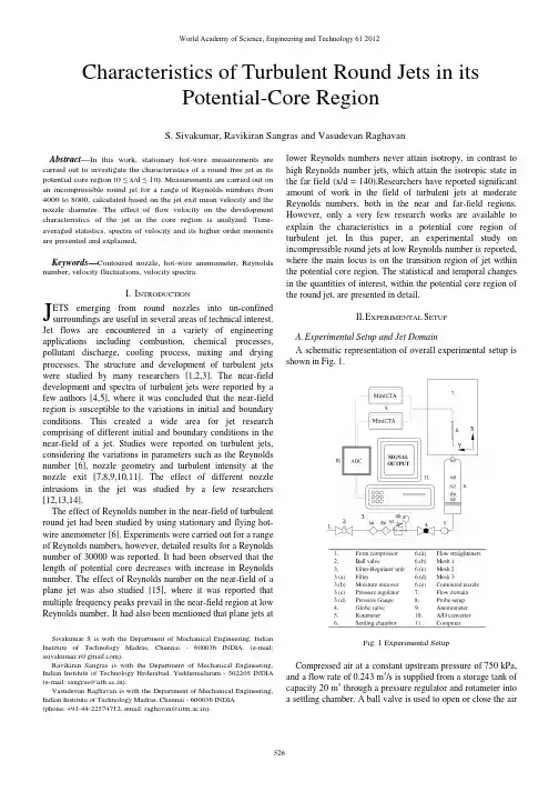
Characteristics of Turbulent Round Jets in its
J
ETS emerging from round nozzles into un-confined surroundings are useful in several areas of technical interest. Jet flows are encountered in a variety of engineering applications including combustion, chemical processes, pollutant discharge, cooling process, mixing and drying processes. The structure and development of turbulent jets were studied by many researchers [1,2,3]. The near-field development and spectra of turbulent jets were reported by a few authors [4,5], where it was concluded that the near-field region is susceptible to the variations in initial and boundary conditions. This created a wide area for jet research comprising of different initial and boundary conditions in the near-field of a jet. Studies were reported on turbulent jets, considering the variations in parameters such as the Reynolds number [6], nozzle geometry and turbulent intensity at the nozzle exit [7,8,9,10,11]. The effect of different nozzle intrusions in the jet was studied by a few researchers [12,13,14]. The effect of Reynolds number in the near-field of turbulent round jet had been studied by using stationary and flying hotwire anemometer [6]. Experiments were carried out for a range of Reynolds numbers, however, detailed results for a Reynolds number of 30000 was reported. It had been observed that the length of potential core decreases with increase in Reynolds number. The effect of Reynolds number on the near-field of a plane jet was also studied [15], where it was reported that multiple frequency peaks prevail in the near-field region at low Reynolds number. It had also been mentioned that plane jets at
Turbulence, magnetic fields and plasma physics in clusters of galaxies
a r X i v :a s t r o -p h /0601246v 2 26 O c t 2006Invited talk,47th APS DPP Meeting,Denver,Oct.24–28,2005;Phys.Plasmas 13,056501(2006)[astro-ph/0601246]Turbulence,magnetic fields and plasma physics in clusters of galaxiesA.A.Schekochihin 1,∗and S.C.Cowley 2,31DAMTP,University of Cambridge,Cambridge CB30WA,UK2Department of Physics and Astronomy,UCLA,Los Angeles,California 90095-15473Plasma Physics Group,Imperial College,Blackett Laboratory,Prince Consort Road,London SW72BW,UK(Dated:February 5,2008)Observations of galaxy clusters show that the intracluster medium (ICM)is likely to be turbulent and is certainly magnetized.The properties of this magnetized turbulence are determined both by fundamental nonlinear magnetohydrodynamic interactions and by the plasma physics of the ICM,which has very low collisionality.Cluster plasma threaded by weak magnetic fields is subject to firehose and mirror instabilities.These saturate and produce fluctuations at the ion gyroscale,which can scatter particles,increasing the effective collision rate and,therefore,the effective Reynolds number of the ICM.A simple way to model this effect is proposed.The model yields a self-accelerating fluctuation dynamo whereby the field grows explosively fast,reaching the observed,dynamically important,field strength in a fraction of the cluster lifetime independent of the exact strength of the seed field.It is suggested that the saturated state of the cluster turbulence is a combination of the conventional isotropic magnetohydrodynamic turbulence,characterized by folded,direction-reversing magnetic fields and an Alfv´e n-wave cascade at collisionless scales.An argument is proposed to constrain the reversal scale of the folded field.The picture that emerges appears to be in qualitative agreement with observations of magnetic fields in clusters.I.INTRODUCTIONClusters of galaxies are vast and varied objects that have long attracted the attention of both observers (in recent decades spectacularly aided by X-ray and radio telescopes)and theoreticians.The observed properties of clusters have proved far from easy to explain as new data has confounded many old theories.The overall budget of the cluster constituents is roughly as follows:∼75%of cluster mass is dark mat-ter,whose sole function is assumed to be to provide the gravitational well,∼20%of cluster mass is the diffuse X-ray-emitting plasma (the intracluster medium,or ICM),while the galaxies have an all but negligible mass.The plasma that makes up the ICM is made of hot and ten-uous ionized hydrogen:temperatures are in the range of 1−10keV,number densities ∼10−1−10−3cm −3,with colder,denser material found in the cool cores and hotter,more diffuse one in the outlying regions.70Necessarily,the first observations and the first the-oretical models of clusters concerned what one might call large-scale features,such as the overall profiles of mass and temperature,the structure formation and the role of the central objects.As observations increased in accuracy and resolution,the ICM was revealed to be much richer than simply a dull cloud of X-ray glow smoothly petering out with distance from the center.A great panoply of features has been detected:bub-bles,filaments,ripples,edges,shocks,sound waves,etc.,as well as very chaotic density,temperature and abun-dance distributions.1,2,3,4,5It is particularly the presence of chaotic fields and the evidence that this chaos exists in a range of scales 4,6,7that makes one expect that ICM,like so many other astrophysical plasmas,is in a turbulent state.It is essential to know the properties of this turbu-lence in order to predict the current and future statisticalmeasurements of the plasma and magnetic fields (spectra,correlation and distribution functions,etc.)and to model correctly the transport processes in the ICM that deter-mine,for example,the overall temperature profiles.8,9We shall assume that the physics of small scales is,at least to some degree,independent of large-scale cir-cumstances and that we can,therefore,gain some use-ful understanding of the turbulence in clusters by ignor-ing large-scale features and considering a homogeneous subvolume of the ICM.In what follows,after reviewing briefly what is known about fluid motions (Sec.II)and magnetic fields (Sec.III)in clusters,we describe,mostly in qualitative terms,what we consider to be the essential aspects of the small-scale physics of the ICM (for plasma physics,see Sec.IV).This will lead us to a tentative overall picture of the structure of the ICM turbulence (Sec.VI)as well as of the origin of its magnetic compo-nent (Sec.V).We must emphasize that the current state of the debates on the nature of turbulence in clusters (and,indeed,on its very existence 10)is such that even a fundamental,conceptual view of the problem has not yet been agreed,and,therefore,a quantitative theory —even an incomplete one such as exists for hydrodynamic turbulence —remains a matter of future work.II.TURBULENCEThe failure of one of the instruments on the ASTRO-E2satellite has set offthe planned direct detection of cluster turbulence 11,12into the (probably not very dis-tant)future.However,indirect evidence of turbulent gas motions does exist:three recent examples are the broad spectrum of pressure fluctuations measured in the Coma cluster 4,detection of subsonic gas motions in the core of the Perseus cluster,13and,again for the Perseus cluster,2TABLE I:Cluster ParametersParameter Expression Cool cores a Hot ICMT observed3×107K108Kn observed6×10−2cm−310−3cm−3v th,i(2T/m i)1/2700km/s1300km/sνii1.5nT−3/2b5×10−13s−12×10−15s−1λmfp v th,i/νii0.05kpc30kpcµ v th,iλmfp1028cm2/s1031cm2/sη3×1013T−3/2b200cm2/s30cm2/sU inferred250km/s300km/sL inferred10kpc200kpcL/U inferred4×107yr7×108yrRe UL/µ 702Rm UL/η4×10276×1029t visc(L/U)Re−1/25×106yr5×108yrl visc L Re−3/40.4kpc100kpcl res L Rm−1/25000km8000kmΩi,eq eB eq/cm i0.3s−10.04s−1ρi,eq v th,i/Ωi,eq3000km30,000kmB0B eqρi,eq/λmfp5×10−17G2×10−19G B1Eq.(13)c3×10−14G2×10−17G B2Eq.(15)c8×10−7G2×10−7GB visc B eq Re−1/49×10−6G4×10−6GB eq(8πm i nU2/2)1/23×10−5G4×10−6Gβeq8πnT/B2eq820l⊥(B2/B eq)L0.2kpc7kpcl B observed1kpc10kpca These numbers are based on the parameters for the Hydra A cluster given in Ref.20.b In these expressions,n is in cm−3,T in Kelvin.c We usedα=3/2to get specific numbers,but the outcome is not very sensitive to the value ofα.the broadening(assumed to be caused by turbulent dif-fusion)of abundance peaks associated with the brightestcluster galaxies.14These and other studies and models based on observational data appear to converge in ex-pecting turbulentflows with rms velocities in the range U∼102−103km/s at the outer scales L∼102kpc. The energy sources for this turbulence are probably the cluster and subcluster merger events and/or,especiallyfor the turbulence in cool cores,the active galactic nu-clei(AGN).The aforementioned observational estimates of the strength and scale of the turbulence are in order-of-magnitude agreement with the outcomes of numerical simulations of cluster formation11,15,16and of the buoy-ant rise of radio bubbles generated by the AGN.17,18Fur-ther discussion and references on the stirring mechanisms for cluster turbulence can be found in Refs.19,20,21. While estimates of the turbulence parameters appear robust roughly to within an order of magnitude,a more quantitative set of numbers is elusive,partly because of the indirect and difficult nature of the observations,partly because the conditions vary both in different clus-ters and within each individual cluster.Here we shalladopt twofiducial sets of parameters:one for cool cores and one for the bulk of hot cluster plasma.These aregiven in Table I(along with some theoretical quantities that will arise in Sec.V and Sec.VI).They will allowus to make estimates that will have the virtue of being consistent and systematic but must not be interpreted asprecise quantitative predictions.They are representative of the range of conditions that can be present in clus-ters.The turbulence is assumed to be stirred at the outer scale L(with rms velocity U at this scale)and to havea Kolmogrov-type cascade below this scale.The small-scale cutoffis determined by the microphysical proper-ties of the cluster plasma.In Table I,we give the value of the particle mean free pathλmfp,which can be usedin a naive estimate of viscosity:µICM∼v th,iλmfp,where v th,i=(2T/m i)1/2is the ion thermal speed.We seethat this gives fairly low values for the Reynolds number, Re∼UL/µICM.It is this feature of the ICM that con-tinues to fuel doubts about its ability to support turbu-lence,at least in the strict,hydrodynamic high-Reynolds-number sense.71However,one should be cognizant of the fact that whatever type of turbulence might exist in the cluster plasma,it is certainly not hydrodynamic,because this plasma is highly electrically conducting72and mag-netized.The presence of the magneticfields not only has a dynamical effect on the turbulence(due to the action of the Lorentz force,the medium acquires a certain elas-tic quality),but also changes the transport properties of the plasma itself:the viscosity,in particular,becomes strongly anisotropic.22These issues will constitute the main subject of this paper,butfirst let us briefly de-scribe what is known about magneticfields in clusters.III.MAGNETIC FIELDSThefirst observed signature of cluster magneticfields was the diffuse synchrotron radio emission in the Coma cluster detected in1970.23Starting from early1990’s, increasingly detailed measurements of the Faraday Ro-tation in the emission from intracluster radio sources have made possible quantitative estimates of the mag-neticfield strength and scales in a large number of clusters.24,25,26Randomly tangled magneticfields with rms strength of order B rms∼1−10µG are consistently found,with thefields in the cool cores of the cooling-flow clusters somewhat stronger than elsewhere.This is fairly close to the value B eq that corresponds to magnetic energy equal to the energy of turbulent motions(see Ta-ble I).Thus,the magneticfield must be dynamically important.The estimates for the tangling scale l B of the field are usually arrived at by assuming that direction reversals along the line of sight(probed by the Faraday Rotation measure)can be described as a random walk with a single step size equal to l B(the estimate of B rms is obtained in conjunction with this model).This gives3 l B∼1−10kpc.The single-scale model is almost certainly not a correctdescription on any but a very rough level.Fortunately,much more detailed information on the spatial structureof the clusterfields is accessible.First,using certain sta-tistical assumptions(most importantly,isotropy),it ispossible to compute magnetic-energy spectra from themaps of the Faraday Rotation measure associated withextended radio sources(the radio lobes of the jets emerg-ing from the AGN—these can be as large as∼102kpcacross).6,27This has been done most thoroughly for a ra-dio lobe located in the cool core of the Hydra A cluster.7The spectrum has a peak at k≃2kpc−1followed bywhat appears to be a power tail consistent with k−5/3down to the resolution limit of k≃10kpc−1.The rmsmagneticfield strength is B rms=7±2µG.The second source of information on the clusterfieldstructure is the polarized synchrotron emission,whichprobes the magneticfield in the plane perpendicular tothe line of sight.28Such data,while widely used for Galac-tic magneticfield studies,29has until recently not beenavailable for clusters.This is now changing:thefirstanalysis of polarized emission from a radio relic in thecluster A2256reveals the presence of magneticfilamentswithfield reversals probably on∼20kpc scale,which,however,is dangerously close to the resolution scale.30 This data is representative of the situation in the bulk of the ICM,rather than in the cores.Statistical analysis of such data will make possible quantitative diagnosis of thefield structure and its dynamical role.31Thus,our knowledge of the magneticfields in clusters, while far from perfect,is more direct and more detailed than that of the turbulent motions of the ICM.It is also due to improve dramatically with the arrival of new radio telescopes such as LOFAR and SKA.73IV.PLASMA PHYSICSThe key property of the ICM as plasma is that it is only weakly collisional and magnetized:given the ob-served values of the magneticfield,the ion gyroradius isρi∼104km,which is much smaller than the mean free path.Asρi≪λmfp already for dynamically veryweakfields(B≫B,see Table I),this is true both inthe observed present state of the ICM and during mostof its hypothetical past,when the magneticfield was be-ing amplified from some weak seed value.In a plasmawithρi≪λmfp,the equations for theflow velocity u and for the magneticfield B may be written in the followingform,valid at time scales≫Ω−1i(Ωi=eB/m i c is the ion cyclotron frequency)and spatial scales≫ρi=v th,i/Ωi,ρd u2 +∇· ˆbˆb p⊥−p +B2 ,(1)d B4πhas been absorbed intoB,and the resistive term has been omitted in Eq.(2)inview of the tiny value of the resistivity.The turbulentmotions in clusters are subsonic(U<v th,i),so we maytake∇·u=0and setρ=1.The magneticfield is,thus,in units of velocity,pressure in units of velocity squared.The proper way to compute p⊥and p is by a kineticcalculation.In the collisional limit,this was done in Bra-ginskii’s classic paper.22It is instructive to obtain hisresult in the following heuristic way that highlights thephysics behind the formalism.32Charged particles mov-ing in a magneticfield conserve theirfirst adiabatic in-variantµ=m i v2⊥/2B.Whenλmfp≫ρi,this conserva-tion is only weakly broken by collisions.As long asµisconserved,any change in thefield strength causes a pro-portional change in p⊥:summing up thefirst adiabaticinvariants of all particles,we get p⊥/B=const.Then1dt∼1dt−νiip⊥−pBdBdt u2 2=−µ |ˆbˆb:∇u|2=−µ 1dt 2 .(5)Thus,the Braginskii viscosity only dissipates such mo-tions that change the strength of the magneticfield.Mo-tions that do not affect B are allowed at subviscous scales.In the weak-field regime,these motions take the form ofplasma instabilities.When the magneticfield is strong,acascade of Alfv´e n waves can be set up below the viscousscale.Let us elaborate.The simplest way to see that pressure anisotropies leadto instabilities is as follows.32Imagine that the large-scaleenergy sources stir up a“fluid”turbulence with u,p⊥,p ,B at time and spatial scales above viscous.Wouldsuch a solution be stable with respect to much higher-frequency and smaller-scale perturbations?Linearizing4 Eq.(1)and denoting perturbations byδ,we get−iωδu=−i k(δp⊥+BδB)+ p⊥−p +B2 δK+iˆb k δp⊥−δp − p⊥−p −B2 δBβ αΩi,(8)whereα=α1+α2>0.This changes the characteristicsof the turbulence:the effective mean free path of theparticles isλmfp,eff∼v th,i/νeff,the effective(parallel)viscosity of the ICM isµ ,eff∼v th,iλmfp,effand,therefore,the effective Reynolds number isRe eff∼UL v2νeff.(9)th,iOn the other hand,using Eq.(4)with effective viscosity,we getµ ,effand|∇u|∼(U/L)Re1/2eff|∆|∼ UαBρi,eq U√B2eqFIG.2:The mechanism of the fluctuation dynamo.Equation (11)models qualitatively the assumed out-come of an as yet inexistent proper theory of the viscos-ity of magnetized ICM.Its solution is plotted inFig.1.Weshalluse this model shortly in our discussion of the fluctuation dynamo in clusters.V.FLUCTUATION DYNAMOIn Sec.III,we reviewed the observational evidence that testified to the presence of a dynamically significant ran-domly tangled magnetic field in clusters.What is the origin of this field?There are numerous physical rea-sons to expect that a certain amount of seed magnetic energy predates structure formation and was,therefore,already present at the birth of clusters.40,41Typical val-ues given for the strength of such field are in the range of B seed ∼10−21−10−17,although this may be an underestimate.42It then falls to the random motions of the cluster plasma to amplify the field to its observed magnitude of a few µG.77This,indeed,they should be able to do by means of the fluctuation (or small-scale)dynamo mechanism:the random stretching of the field.It is a fundamental property of a succession of random (in time)linear shears that it leads on the average to expo-nential growth of the energy of the magnetic field frozen into the medium.43,44,45The rate of growth is roughly equal to the rate of strain (shear,or stretching rate)of the random flow.While the mathematical theory of this process can be nontrivial,46the physics of it is basically illustrated by Fig.2.In Kolmogorov turbulence,the rate of strain is domi-nated by the viscous scale,so |∇u |∼t −1visc∼(U/L )Re 1/2.In fact,what is relevant for the growth of the magnetic field is not the full rate-of-strain tensor but its “paral-lel”component,ˆbˆb :∇u .Since this is exactly the type of motion damped by Braginskii viscosity [see Eqs.(4–5)],we can,for the purposes of the fluctuation dynamo,ignore any subviscous-scale velocity fluctuations.Thus,the magnetic field should grow according to 781dt=ˆbˆb :∇u ∼U Lv th ,i(1−t/t c )2+α,(14)where B (0)∼the greater of B seed and B 1and t c =(2+α)(L/U )Re −1/2[B 1/B (0)]1/(2+α)is at most (for B seed <B 1)the viscous turnover time t visc associated with the collisional Re.The explosive stage contin-ues until the amplified field starts suppressing the in-stabilities,i.e.,when βdrops to values comparable to(v th ,i /U )2Re 1/2eff.This happens at B ∼B 2,whereB 2=B eqv th ,iL1/(5+2α).(15)Thus,we have a mechanism that amplifies the field by many orders of magnitude from any strength above B 1to B 2in finite,cosmologically short,time ∼t c .The value of B 2turns out to be only just over an order of magnitude below B eq (see Table I).Further growth of the field is algebraically slow (B ∼t 1/2),but it does not have to go on for a very long time because B 2is already quite close to the observed field strength.To be precise,there are two algebraic regimes.During the first,Re effis still controlled by thesecond term in Eq.(11)as B hovers just below B eq Re −1/4effwhile B is increasing and Re effis decreasing.Eventually,B ∼B visc =B eq Re −1/4and Re effis returned back to Re (plasma instabilities are suppressed).79As this is also the field strength at which the field has energy comparable to the energy of the viscous-scale motions,any further growth of the field is a nonlinear process,in which the back reaction of the field on the flow has to be taken intoFIG.3:Evolution of the magnetic-field strength for the cool-core parameters of Table I.account.This can be done by assuming that,as thefield grows,it can no longer be stretched by motions whose energy it exceeds and that,therefore,at any given time, the dominant stretching is exerted by motions whose en-ergy is equal to that of thefield.Denoting their velocity and scale by u l and l and using u2l∼B2,we have58,59 dB2∼u3ll1−A 1FIG.5:A schematic illustration of the structure of cluster turbulence proposed in Sec.VI.ratio l /l⊥,the larger is the contrast between the strong field in the straight segments of the folds and the weakfield in the corners.We assume that the rms value of thefield is determined by the straight segments becausethese are thefields that are stretched by turbulence.It istheir growth that we studied in Sec.V.In the saturated state,we expect B straight∼B eq.For such a strongfield, the plasma instabilities are suppressed.It is intuitively clear that they must be suppressed in the regions of theweakfield as well,i.e.,thefield there cannot be weaker than B2[Eq.(15)].Indeed,as we saw in Sec.V,the explosive dynamo mechanism brings anyfield up to this value nearly instantaneously(for B>B2,the growth is much slower).We may conjecture that the maximum aspect ratio of the folds is set by the maximum contrast in thefield strength l /l⊥∼B eq/B2.81Substituting the numbers,wefind(Table I)that this prediction gives the field reversal scale no smaller than a few per cent of the outer scale L(taking l ∼L).This is in passable agree-ment with the observational evidence,which is the best one can expect,given the highly imprecise nature of our argument,of most observational inferences,and of the definitions of such quantities as l B,l⊥,l and L.For comparison of our model with observational data for a number of individual clusters,see Ref.20.It is fair to acknowledge that the above argument,while providing a useful constraint,falls short of a sat-isfactory explanation of thefield structure.One might argue that if,in the course of the turbulent stretch-ing/shearing of thefield,a region offield strength below B2appears(as explained above,in the corner of a fold), Re effthere becomes very large and a localized spot of high-Reynolds-number turbulence is formed.This should have two principal effects.Thefirst is akin to that of a locally enhanced turbulent resistivity,so thefield that violates our constraint is continuously destroyed.The second is a burst of explosivefluctuation dynamo in the spot,which produces more foldedfield with B>B2 and thus shuts itself down.These folds are then further stretched,sheared,etc.,again subject to the constraint that they are destroyed and replaced by new ones wher-ever a spot of weakfield appears.We do not currently have a more detailed mechanistic scenario of how exactly the folded structure with l /l⊥∼B eq/B2is established. It may be feasible to test these ideas numerically by solv-ing MHD equations with viscosity locally determined by the magnetic-field strength according to Eq.(11).Let us assume that clusterfields do indeed have a folded structure with a direction reversal scale l⊥∼(0.01...0.1)L,possibly determined by the argument given above.82The magnetic-energy spectrum then peaks at k∼1/l⊥.What is the structure of the turbulence above and below this scale?At scales l≪l⊥,the magnetic field reversing at the scale l⊥will appear uniform and,in accordance with the old idea of Kraichnan63could sup-port a cascade of Alfv´e n waves.This cascade can rig-orously be shown to be described by the equations of Reduced MHD at collisionless scales all the way down to the ion gyroscale.37The currently accepted theory of such a cascade,primarily associated with the names of Goldreich and Sridhar,64is based on the conjecture that at each scale,the Alfv´e n frequency is equal to the turbu-lent decorrelation rate.The result is a k−5/3spectrum of Alfv´e nicfluctuations—this possibly explains what ap-pears to be a k−5/3tail in the observed spectrum of mag-netic energy for the Hydra A core.7We cannot embark on a detailed discussion of the theory of the Alfv´e n-wave cascade here,so the reader is referred to Ref.65for a re-view and to Ref.37for the theoretical basis of extending this theory to collisionless scales.Above the reversal scale,l≫l⊥,the cluster turbu-lence should resemble the saturated state of isotropic MHD turbulence:a magnetic-energy spectrum with a positive spectral index corresponding to foldedfields and a kinetic-energy spectrum populated in the inertial range by a peculiar type of Alfv´e n waves that propagate along the folds(i.e.,simultaneously perturbing the antiparallel magneticfield lines).58,59This type of turbulence is also reviewed in Ref.65.It is probably of limited relevance for clusters because the Reynolds number in the ICM is not large enough to allow a well-developed inertial range. Fig.5summarizes the—admittedly,rather specula-tive—picture of cluster turbulence proposed above.We offer this sketch in lieu of conclusions.While we believe that the set of physical arguments that has led to it is not without merit,it is clear that much analytical,numeri-cal and observational work is needed before a conclusion can truly be reached in the study of turbulence,magnetic fields and plasma physics in clusters of galaxies.AcknowledgmentsHelpful discussions with T.Enßlin,G.Hammett, R.Kulsrud,E.Quataert,and P.Sharma are gratefully acknowledged.This work was supported by a UKAFF Fellowship,a PPARC Advanced Fellowship,King’s Col-lege,Cambridge(A.A.S.)and by the DOE Center for Multiscale Plasma Dynamics. A.A.S.also thanks the Royal Society(UK)and the APS for travel support.∗Electronic address:as629@1A.C.Fabian,J.S.Sanders,S.W.Allen,C.S.Crawford, K.Iwasawa,R.M.Johnstone,R.W.Schmidt,and G.B.Taylor,Mon.Not.R.Astron.Soc.344,L43(2003).2A.C.Fabian,J.S.Sanders,G.B.Taylor,S.W.Allen,C.S.Crawford,R.M.Johnstone,and K.Iwasawa,Mon.Not.R.Astron.Soc.366,417(2006).3A.C.Fabian,J.S.Sanders,G.B.Taylor,and S.W.Allen,Mon.Not.R.Astron.Soc.(2005),in press(astro-ph/0503154).4P.Schuecker,A.Finoguenov,F.Miniati,H.B¨o hringer, and U.G.Briel,Astron.Astrophys.426,387(2004).5E.Churazov,W.Forman, C.Jones,and H.B¨o hringer, Astrophys.J.590,225(2003).6C.Vogt and T.A.Enßlin,Astron.Astrophys.412,373 (2003).7C.Vogt and T.A.Enßlin,Astron.Astrophys.434,67 (2005).8T.J.Dennis and B.D.G.Chandran,Astrophys.J.622, 205(2005).9L.M.Voigt and A.C.Fabian,Mon.Not.R.Astron.Soc.347,1130(2004).10A.C.Fabian,J.S.Sanders,C.S.Crawford,C.J.Con-selice,J.S.Gallagher,and R.F.G.Wyse,Mon.Not.R.Astron.Soc.344,L48(2003).11R.A.Sunyaev,M.L.Norman,and G.A.Bryan,Astron.Lett.29,783(2003).12N.A.Inogamov and R.A.Sunyaev,Astron.Lett.29,791 (2003).13E.Churazov,W.Forman, C.Jones,R.Sunyaev,andH.B¨o hringer,Mon.Not.R.Astron.Soc.347,29(2004). 14P.Rebusco,E.Churazov,H.B¨o hringer,and W.Forman, Mon.Not.R.Astron.Soc.359,1041(2005).15M.L.Norman and G.L.Bryan,Lect.Notes Phys.530, 106(1999).16P.M.Ricker and C.L.Sarazin,Astrophys.J.561,621 (2001).17Y.Fujita,Astrophys.J.631,L17(2005).18E.Churazov,M.Br¨u ggen,C.R.Kaiser,H.B¨o hringer,and W.Forman,Astrophys.J.554,261(2001).19K.Subramanian,A.Shukurov,and N.E.L.Haugen,Mon.Not.R.Astron.Soc.366,143(2006).20T.A.Enßlin and C.Vogt,Astron.Astrophys.(2006),in press(astro-ph/0505517).21B.D.G.Chandran,Astrophys.J.632,809(2005).22S.I.Braginskii,Rev.Plasma Phys.1,205(1965).23M.A.G.Willson,Mon.Not.R.Astron.Soc.151,1(1970). 24P.P.Kronberg,Rep.Prog.Phys.57,325(1994).25C.L.Carilli and G.B.Taylor,Ann.Rev.Astron.Astro-phys.40,319(2002).oni and L.Feretti,Int.J.Mod.Phys.D13,1549 (2004).27T.A.Enßlin and C.Vogt,Astron.Astrophys.401,835 (2003).28B.J.Burn,Mon.Not.R.Astron.Soc.133,67(1966). 29M.Haverkorn,P.Katgert,and A.G.de Bruyn,Astron.Astrophys.403,1045(2003).30T.E.Clarke and T.A.Enßlin,Astron.J.(2006),in press (astro-ph/0603166).31T.A.Enßlin,A.Waelkens,C.Vogt,and A.A.Schekochi-hin,Astron.Nachr.327,626(2006).32A.A.Schekochihin,S.C.Cowley,R.M.Kulsrud,G.W.Hammett,and P.Sharma,Astrophys.J.629,139(2005). 33M.N.Rosenbluth(1956),Los Alamos Scientific Labora-tory Report LA-2030.34S.Chandrasekhar,A.N.Kaufman,and K.M.Watson, Proc.R.Soc.London,Ser.A245,435(1958).35E.N.Parker,Phys.Rev.109,1874(1958).36A.A.Vedenov and R.Z.Sagdeev,Sov.Phys.Doklady3, 278(1958).37A.A.Schekochihin,S.C.Cowley,W.D.Dorland,G.W.Hammett,G.G.Howes,and E.Quataert,Astrophys.J.(2006),submitted.38V.D.Shapiro and V.L.Shevchenko,Sov.Phys.JETP18, 1109(1964).39K.B.Quest and V.D.Shapiro,J.Geophys.Res.101, 24457(1996).40D.Grasso and H.R.Rubinstein,Phys.Rep.348,163 (2001).41N.Y.Gnedin,A.Ferrara,and E.Zweibel,Astrophys.J.539,505(2000).42R.Banerjee and K.Jedamzik,Phys.Rev.Lett.91,251301 (2003).43G.K.Batchelor,Proc.R.Soc.London,Ser.A201,405 (1950).44Y.B.Zeldovich,A.A.Ruzmaikin,S.A.Molchanov,andD.D.Sokoloff,J.Fluid Mech.144,1(1984).45Y.B.Zeldovich,A.A.Ruzmaikin,and D.D.Sokoloff,The Almighty Chance(World Scientific,Singapore,1990).46V.I.Arnold and B.A.Khesin,Topological Methods in Hydrodynamics(Springer,Berlin,1999).47W.Jaffe,Astrophys.J.241,925(1980).48J.Roland,Astron.Astrophys.93,407(1981).49A.Ruzmaikin,D.Sokoloff,and A.Shukurov,Mon.Not.R.Astron.Soc.241,1(1989).50D.S.D.Young,Astrophys.J.386,464(1992).51O.Goldshmidt and Y.Rephaeli,Astrophys.J.411,518 (1993).52F.J.S´a nchez-Salcedo,A.Brandenburg,and A.Shukurov, Astrophys.Space Sci.263,87(1998).53K.Roettinger,J.M.Stone,and J.O.Burns,Astrophys.J.518,594(1999).54K.Dolag,M.Bartelmann,and H.Lesch,Astron.Astro-phys.348,351(1999).55K.Dolag,M.Bartelmann,and H.Lesch,Astron.Astro-phys.387,383(2002).56K.Dolag,D.Grasso,V.Springel,and achev,J.Cos-mol.Astropart.Phys.1,9(2005).57M.Br¨u ggen,M.Ruszkowski,A.Simonescu,M.Hoeft,andC.Dalla Vecchia,Astrophys.J.631,L21(2005).58A.A.Schekochihin,S.C.Cowley,G.W.Hammett,J.L.Maron,and J.C.MacWilliams,New J.Phys.4,84(2002). 59A. A.Schekochihin,S. C.Cowley,S. F.Taylor,J.L.Maron,and J.C.MacWilliams,Astrophys.J.612,276 (2004).60E.Ott,Phys.Plasmas5,1636(1998).61A.Schekochihin,S.Cowley,J.Maron,and L.Malyshkin, Phys.Rev.E65,016305(2002).62A.Brandenburg and K.Subramanian,Phys.Rep.417,1 (2005).63R.H.Kraichnan,Phys.Fluids8,1385(1965).64P.Goldreich and S.Sridhar,Astrophys.J.438,763(1995).。
半导体物理与器件——Terms汉译英
半导体物理与器件——Terms(术语)U1 Terms:Semiconductor physics and devices半导体物理与器件,Space lattice空间晶格, unit cell晶胞, primitive cell原胞,basic crystal structures 基本晶格结构(five), Miller indices密勒指数, atomic bonding原子价键U2 Terms:quantum mechanics量子力学,energy quanta能量子, wave-particle duality波粒二象性,the uncertainty principle测不准原理/海森堡不确定原理Schrodinger's wave equation薛定谔波动方程, eletrons in free Space自由空间中的电子the infinite potential well无限深势阱, the step potential function 阶跃势函数, the potential barrier势垒.U3 Terms:Pauli exclusion principle泡利不相容原理, quantum state量子态. allowed energy band允带, forbidden energy band禁带.conduction band导带, valence band价带,hole空穴, electron 电子.effective mass有效质量.density of states function状态密度函数,the Fermi-Dirac probability function费米-狄拉克概率函数,the Boltzmann approximation波尔兹曼近似,the Fermi energy费米能级.U4 Terms:charge carriers载流子, effective density of states function有效状态密度函数,intrinsic本征的,the intrinsic carrier concentration本征载流子浓度, the intrinsic Fermi level本征费米能级.charge neutrality电中性状态, compensated semiconductor补偿半导体, degenerate简并的,non-degenerate非简并的, position of E F费米能级的位置U5 Terms:drift current漂移电流, diffusion current 扩散电流,mobility迁移率, lattice scattering晶格散射, ionized impurity scattering 电离杂质散射, velocity saturation饱和速度,conductivity电导率,resistivity电阻率.graded impurity distribution杂质梯度分布,the induced electric field感生电场, the Einstein relation爱因斯坦关系, the hall effect霍尔效应U6 Terms:nonequilibrium excess carriers非平衡过剩载流子,carrier generation and recombination载流子的产生与复合,excess minority carrier过剩少子,lifetime寿命,low-level injection小注入,ambipolar transport双极输运, quasi-Fermi energy准费米能级.U7 Terms:the space charge region空间电荷区,the built-in potential内建电势, the built-in potential barrier内建电势差,the space charge width空间电荷区宽度, zero applied bias零偏压, reverse applied bias反偏, onesided junction单边突变结.U8 Terms:the PN junction diode PN结二极管, minority carrier distribution少数载流子分布, the ideal-diode equation理想二极管方程, the reverse saturation current density反向饱和电流密度.a short diode短二极管,generation-recombination current产生-复合电流,the Zener effect齐纳效应, the avalanche effect雪崩效应, breakdown击穿.U9 Terms:Schottky barrier diode (SBD)肖特基势垒二极管,Schottky barrier height肖特基势垒高度.Ohomic contact欧姆接触,heterojunction异质结, homojunction单质结,turn-on voltage开启电压,narrow-bandgap窄带隙, wide-bandgap宽带隙,2-D electron gas二维电子气U10 Terms:bipolar transistor双极晶体管,base基极, emitter发射极, collector集电极.forward active region正向有源区, inverse active region反向有源区, cut-off截止, saturation饱和,current gain电流增益,common-base共基, common-emitter共射.base width modulation基区宽度调制效应, Early effect厄利效应, Early voltage厄利电压U11 Terms:Gate栅极, source源极, drain漏极, substrate基底.work function difference功函数差threshold voltage阈值电压, flat-band voltage平带电压enhancement mode增强型, depletion mode耗尽型strong inversion强反型, weak inversion弱反型,transconductance跨导, I-V relationship电流-电压关系。
湍流长度尺度英文
湍流长度尺度英文Turbulence Length ScalesTurbulence is a complex and fascinating phenomenon that has been the subject of extensive research and study in the field of fluid mechanics. One of the key aspects of turbulence is the concept of turbulence length scales, which refers to the range of different-sized eddies or vortices that are present in a turbulent flow. These length scales play a crucial role in understanding and predicting the behavior of turbulent flows, and they have important implications in a wide range of engineering and scientific applications.The smallest length scale in a turbulent flow is known as the Kolmogorov length scale, named after the Russian mathematician and physicist Andrey Kolmogorov. This length scale represents the size of the smallest eddies or vortices in the flow, and it is determined by the rate of energy dissipation and the kinematic viscosity of the fluid. The Kolmogorov length scale is typically denoted by the Greek letter η (eta) and can be expressed as η = (ν^3/ε)^(1/4), where ν is the kinematic viscosity of the fluid and ε is the rate of energy dissipation.The Kolmogorov length scale is important because it represents the scale at which viscous forces become dominant and energy is dissipated into heat. Below this length scale, the flow is considered to be in the dissipation range, where the eddies are too small to sustain their own motion and are rapidly broken down by viscous forces. The Kolmogorov length scale is therefore a critical parameter in the study of turbulence, as it helps to define the range of scales over which energy is transferred and dissipated within the flow.Another important length scale in turbulence is the integral length scale, which represents the size of the largest eddies or vortices in the flow. The integral length scale is typically denoted by the symbol L and is a measure of the size of the energy-containing eddies, which are responsible for the bulk of the turbulent kinetic energy in the flow. The integral length scale is often determined by the geometry of the flow domain or the boundary conditions, and it can be used to estimate the overall scale of the turbulent motion.Between the Kolmogorov length scale and the integral length scale, there is a range of intermediate length scales known as the inertial subrange. This range is characterized by the presence of eddies that are large enough to be unaffected by viscous forces, but small enough to be unaffected by the large-scale features of the flow. In this inertial subrange, the energy is transferred from the large eddies to the smaller eddies through a process known as the energycascade, where energy is transferred from larger scales to smaller scales without significant dissipation.The energy cascade is a fundamental concept in turbulence theory and is described by Kolmogorov's famous 1941 theory, which predicts that the energy spectrum in the inertial subrange should follow a power law with a slope of -5/3. This power law relationship has been extensively verified through experimental and numerical studies, and it has important implications for the modeling and prediction of turbulent flows.In addition to the Kolmogorov and integral length scales, there are other important length scales in turbulence that are relevant to specific applications or flow regimes. For example, in wall-bounded flows, the viscous length scale and the boundary layer thickness are important parameters that can influence the turbulent structure and behavior. In compressible flows, the Taylor microscale and the Corrsin scale are also relevant length scales that can provide insight into the characteristics of the turbulence.The understanding of turbulence length scales is crucial for a wide range of engineering and scientific applications, including fluid dynamics, aerodynamics, meteorology, oceanography, and astrophysics. By understanding the different length scales and their relationships, researchers and engineers can better predict andmodel the behavior of turbulent flows, leading to improved designs, more accurate simulations, and a deeper understanding of the fundamental principles of fluid mechanics.In conclusion, turbulence length scales are a fundamental concept in the study of turbulent flows, and they play a crucial role in our understanding and modeling of this complex and fascinating phenomenon. From the Kolmogorov length scale to the integral length scale and the inertial subrange, these length scales provide valuable insights into the structure and dynamics of turbulence, and they continue to be an active area of research and exploration in the field of fluid mechanics.。
湍流燃烧模型
Contents
1. Introduction . . . . . . . . . . . . . . . . . . . . . . . . . . . . . . . . . . . . . . . . . . . . . . . . . . . . . . . . . . . . . . . . . . 195 2. Balance equations . . . . . . . . . . . . . . . . . . . . . . . . . . . . . . . . . . . . . . . . . . . . . . . . . . . . . . . . . . . . . . 196
194
D. Veynante, L. Vervisch / Progress in Energy and Combustion Science 28 (2002) 193±266
6. Tools for turbulent combustion modeling . . . . . . . . . . . . . . . . . . . . . . . . . . . . . . . . . . . . . . . . . . . . . 212 6.1. Introduction . . . . . . . . . . . . . . . . . . . . . . . . . . . . . . . . . . . . . . . . . . . . . . . . . . . . . . . . . . . . . . 212 6.2. Scalar dissipation rate . . . . . . . . . . . . . . . . . . . . . . . . . . . . . . . . . . . . . . . . . . . . . . . . . . . . . . . 214 6.3. Geometrical description . . . . . . . . . . . . . . . . . . . . . . . . . . . . . . . . . . . . . . . . . . . . . . . . . . . . . . 214 6.3.1. G-®eld equation . . . . . . . . . . . . . . . . . . . . . . . . . . . . . . . . . . . . . . . . . . . . . . . . . . . . . 214 6.3.2. Flame surface density description . . . . . . . . . . . . . . . . . . . . . . . . . . . . . . . . . . . . . . . . . 216 6.3.3. Flame wrinkling description . . . . . . . . . . . . . . . . . . . . . . . . . . . . . . . . . . . . . . . . . . . . . 218 6.4. Statistical approaches: probability density function . . . . . . . . . . . . . . . . . . . . . . . . . . . . . . . . . . 218 6.4.1. Introduction . . . . . . . . . . . . . . . . . . . . . . . . . . . . . . . . . . . . . . . . . . . . . . . . . . . . . . . . 218 6.4.2. Presumed probability density functions . . . . . . . . . . . . . . . . . . . . . . . . . . . . . . . . . . . . 219 6.4.3. Pdf balance equation . . . . . . . . . . . . . . . . . . . . . . . . . . . . . . . . . . . . . . . . . . . . . . . . . . 219 6.4.4. Joint velocity/concentrations pdf . . . . . . . . . . . . . . . . . . . . . . . . . . . . . . . . . . . . . . . . . 221 6.4.5. Conditional moment closure (CMC) . . . . . . . . . . . . . . . . . . . . . . . . . . . . . . . . . . . . . . . 221 6.5. Similarities and links between the tools . . . . . . . . . . . . . . . . . . . . . . . . . . . . . . . . . . . . . . . . . . 221
- 1、下载文档前请自行甄别文档内容的完整性,平台不提供额外的编辑、内容补充、找答案等附加服务。
- 2、"仅部分预览"的文档,不可在线预览部分如存在完整性等问题,可反馈申请退款(可完整预览的文档不适用该条件!)。
- 3、如文档侵犯您的权益,请联系客服反馈,我们会尽快为您处理(人工客服工作时间:9:00-18:30)。
a r X i v :0803.1689v 1 [a s t r o -p h ] 12 M a r 2008The effect of turbulent intermittency on the deflagration todetonation transition in SN Ia explosionsLiubin Pan,J.Craig Wheeler and John ScaloAstronomy Department,University of Texas at Austinpanlb@ ABSTRACT We examine the effects of turbulent intermittency on the deflagration to det-onation transition (DDT)in Type Ia supernovae.The Zel’dovich mechanism for DDT requires the formation of a nearly isothermal region of mixed ash and fuel that is larger than a critical size.We primarily consider the hypothesis by Khokhlov et al.and Niemeyer and Woosley that the nearly isothermal,mixed region is produced when the flame makes the transition to the distributed regime.We use two models for the distribution of the turbulent velocity fluctuations to estimate the probability as a function of the density in the exploding white dwarf that a given region of critical size is in the distributed regime due to strong local turbulent stretching of the flame structure.We also estimate lower limits on the number of such regions as a function of density.We find that the distributed regime,and hence perhaps DDT,occurs in a local region of critical size at a density at least a factor of 2−3larger than predicted for mean conditions that neglect intermittency.This factor brings the transition density to be much larger than the empirical value from observations in most situations.We also consider the intermittency effect on the more stringent conditions for DDT by Lisewski et al.and Woosley.We find that a turbulent velocity of 108cm/s in a region of size 106cm,required by Lisewski et al.,is rare.We expect that intermittency givesa weaker effect on the Woosley model with stronger criterion.The predicted transition density from this criterion remains below 107g/cm 3after accounting for intermittency using our intermittency models.Subject headings:stars:interiors—supernovae:general—turbulence1.IntroductionA successful model for Type Ia Supernova (SNIa)explosions is required to produce a de-flagration to detonation transition (DDT)by observational constraints.A pure deflagrationmodel gives exploding kinetic energy lower than observed(Khokhlov1991;Gamezo et al. 2003;R¨o pke&Hillebrandt2005)and pure detonation leads to overproduction of iron group elements and too little intermediate elements(Branch et al.1982,1983).The densityρtr at which the transition occurs determines the amount of the nickel produced(H¨oflich1995; H¨oflich and Khokhlov1996;Dominguez,H¨oflich&Straniero2001).Therefore a prediction ofρtr,consistent with the observed nickel production,is essential to a DDT theory for SNe Ia.The mechanism by which the DDT occurs still remains a mystery.The most studied candidate is the Zel’dovich mechanism,which requires the existence of an almost isother-mal region of mixed ash and fuel that is larger than a critical size l c to drive a supersonic shock that is sufficiently strong to sweep over the entire star(Khokhlov et al.1997,here-after KOW;Niemeyer and Woosley1997,hereafter NW).One hypothesis is that a nearly isothermal region is produced by turbulent preconditioning.KOW argued that,to produce an almost isothermal mixture of ash and fuel,the laminarflame must be quenched by tur-bulent stretching,at least locally.This might allow the cold fuel to mix with the ash both thermally by electron conduction and chemically by diffusivity without being burned.They assumed that the criterion to quench aflame is that the turbulent velocity at the laminar flame thickness must be larger than the laminarflame speed.NW gave a similar argument based on the distributedflame burning regime in turbulent combustion.The criterion for a distributedflame is expressed in terms of the Gibson scale at which the turbulence velocity equals the laminarflame speed.If the Gibson scale is smaller than the laminarflame thick-ness,turbulent stretching can generate structures within theflame and theflame is in the distributed regime.NW speculated that in this regimeflames can be temporally quenched in some regions,which can host the detonation after being homogenized in temperature and composition by turbulent mixing.The criterion for the distributed regime is equivalent to that forflame quenching used by KOW.Both criteria give the same condition on the turbu-lence intensity for given laminarflame properties(see§2).As the density in the star drops due to the overall expansion,it is easier for turbulence to affect the laminarflame because of the decrease in theflame speed and the increase inflame thickness.With presumed tur-bulence parameters,the criterion for the turbulence intensity,determined by the robustness of laminarflames disturbed by turbulent motions,translates to a transition densityρtr for the DDT.Several uncertainties exist in the simple model given by these two early studies.First, it is not clear whether the criterion used by KOW,equivalent to that for a distributed regime(NW),is sufficient forflame breaking.How,or even if,flames are quenched is still an open question.Second,it is uncertain whether(local)flame quenching is indeed necessary to produce a nearly isothermal region.Finally,later studies by Lisewski,Hillebrandt andWoosley(2000)(hereafter Lisewski et al2000;see also Lisewski et al.2000b)and Woosley (2007)find that entering the distributed regime,while probably a necessary condition,is not sufficient for the DDT to occur.Based on a requirement for turbulent transport to be efficient at producing a shallow temperature and composition gradient around the laminar flame,Lisewski et al.(2000)find that the turbulent velocity at the scale106cm needed for a detonation is very large,∼108cm/s.Woosley(2007)claims that the DDT occurs only when the turbulentflame thickness exceeds a critical length scale.We show in§2that the two criteria,although arising from different physical considerations,are basically equivalent. The corresponding condition is more stringent than that assumed by KOW and NW.In this paper we examine the effect of turbulent intermittency on the onset of distributed burning that may relate to the DDT.Despite the uncertainties listed above,we will mainly consider the model by KOW and NW and use it to illustrate the potential importance of intermittency in SN Ia explosions.Our calculations can be applied to the criteria by Lisewski et al.(2000)and Woosley(2007)in a straightforward way.A quantitative analysis using their criteria requires data for laminarflame properties and critical length scales at densities below107g cm−3that are not immediately available(see§2).We give a qualitative discussion of the intermittency effect on their DDT models.Intermittency is an important concept in turbulence theory.It is characterized by intense local events,e.g.,strong stretching at small scales,which occur at a frequency much larger than predicted from a Gaussian distribution(see,e.g.,Frisch1995).The physical origin of intermittency in turbulentflows is the spatial inhomogeneity in the energy dissipation rate: most kinetic energy is viscously dissipated in thefinest structures,e.g.,vortex tubes,which occupy only a small volume fraction.These rare but intense dissipative structures give rise to a spatially inhomogeneous and intermittent distribution for the turbulent intensity and the stretching rate.Intermittency is shown as broad exponential tails in the probability distribution for the stretching rate or the dissipation rate at small scales(see§3).The tails get broader at smaller scales,meaning that the probability offinding an extreme turbulent stretching rate or intensity increases with decreasing scales.According to1D simulation results by KOW and NW,the critical size,l c,of the isother-mal region required for a DDT via the Zel’dovich mechanism is much smaller,especially at large densities,than the expected integral length scale for the buoyancy-driven turbulence in SN Ia explosions.This suggests that only a smallflame region with a sufficiently strong local turbulence intensity may be needed to trigger a detonation.Turbulent intermittency, which indicates the existence of regions of small sizes where the turbulent stretching is much larger than the average value over theflow,is therefore expected to have important conse-quences for DDT.The transition could happen earlier at a higher transition densityρtr thanpredicted by models using the average turbulent intensity.At higher densities,much larger turbulent intensity is required for the DDT,but the rapid decrease of l c with increasing den-sity makes an earlier DDT possible for two reasons.First,the probability is larger tofind regions of smaller sizes l c with extreme turbulent stretching rate or intensity.Second,there are more regions of smaller size available as candidates to host the detonation.Clearly,the intermittency effect accounts for the intuitive dependence ofρtr on l c:the smaller the critical size,the easier it may be for the transition to happen.To what degree the intermittency effect increasesρtr is the main question we investigate in this paper.In§2,we review the criteria for the DDT in models by KOW,NW,Lisewski et al. (2007)and Woosley(2007)and formulate a new criterion taking into account the effect of intermittency.We describe two intermittency models by Oboukhov(1962)and Kolmogorov (1962)and by She and Leveque(1994)in§ing the intermittency models,we evaluate the transition density from the new criteria in§4.Our results are summarized and discussed in§5.2.Criteria for the DDTThe criterion used in NW for judging whether aflame is in the distributed regime,which was also assumed to be the condition for the DDT,is to compare the Gibson scale l G with the laminarflame thickness l f.The Gibson scale is defined such thatδu(l G)=S l whereδu(l)is the amplitude of the velocityfluctuations at the scale l(or equivalently the velocity difference over a scale l,i.e.,δu(l)=u(l+x)−u(x))and S l is the laminarflame speed1.If l G∼>l f, the turbulence cannot internally disturb theflame and the turbulence in effect wrinkles the flame.This is called theflamelet regime.Only when l G∼<l f,can turbulence stretch the flame efficiently to generate structures within theflame and the turbulent combustion enters the distributed regime.The condition l G∼<l f is equivalent toδu(l f)∼>δu(l G)=S l since δu(l)is an increasing function of the scale l2.The latter,which means that the turbulentvelocityfluctuationδu(l f)at the scale of theflame thickness l f is larger than the laminar flame speed,is the criterion used in KOW forflame quenching and the DDT.Following KOW,we introduce a factor of K∼1in the criterion to account for the uncertainty in theflame breaking mechanism,i.e.,δu(l f)≥KS l.We will consider two values for K,i.e.,K=1and K=8(KOW;For K=8,to quench aflame,the Gibson scale has to be K3=512times smaller than theflame width).This criterion can also be written in terms of timescales.Noting that the turbulent stretching timescale,τt,at the flame thickness isτt(l f)=l f/δu(l f)and that the nuclear reaction timescale,τn,is related to theflame speedτn=l f/S l,the criterion is equivalent toτt(l f)<τn/K,i.e.,to break theflame the stretching timescale at theflame thickness must be smaller than the nuclear burning timescale(see Niemeyer and Kerstein1997).To apply this criterion,the Kolmogorov(1941)scalingδu(l)=¯ǫ1/3l1/3is usually used to calculateδu(l f)from the turbulent velocityfluctuations at large scales where¯ǫis the average dissipation rate in theflow.From this scaling,the criterion can be written as(KOW,NW),>KS l(1)¯ǫ1/3l1/3for¯ǫ>K3S3l/l f=K3ǫf(2) whereǫf is defined as S3l/l f.Although we use the convenient criterion(2)in terms of the dissipation rate in our calculations,the turbulent stretching is more fundamental and we will use the concept of theflame stretching in our discussions.The laminarflame speed and thickness depend on the chemical composition and the density(Timmes and Woosley1992,KOW).In Table1,we list theflame speed,theflame thickness as a function of density for a white dwarf with half carbon and half oxygen,mainly taken from Timmes and Woosley(1992).The laminar speed decreases and the thickness increases quickly with decreasing densityρ,thereforeǫf decreases rapidly with decreasing ρas shown in Table1.The average dissipation rate is estimated to be¯ǫ=U3/L where U and L are the characteristic velocity and length scales of the turbulence,normally set by motions on the large,driving scale.At large scales,the turbulence is driven by the Rayleigh-Taylor instability.The length scale L might be expected to be about the size,R f, of theflame region,L≃R f∼108cm and the velocity scale to be about the Rayleigh-Taylor velocity at this scale U∼0.5respectively,are not equivalent.scales larger than106cm freeze out due to the overall expansion of the star.In that case, L∼106−107cm and U∼107cm/s.We will take U and L as parameters.Note that the criterion eq(2)depends on U and L through the dissipation rate.Given the dissipation rate ¯ǫ,the critical density below which the inequality(eq2)is satisfied can be obtained using ǫf as a function ofρin Table1.For example,if U∼100km/s and L∼100km,¯ǫ∼1014 cm2/s3and wefind that,from interpolation in Table1,¯ǫis larger thanǫf at a density less than∼4×10⁷g/cm3.Therefore criterion(2)predicts a transition densityρtr≃4×10⁷ g/cm3for K=1(see KOW and NW).If K=8,the predicted transition density is smaller,ρtr∼1.5×10⁷g/cm3.In the second line of Table2,we give the predictedρtr for different values of the parameters,which decreases with decreasing dissipation rate¯ǫ.The numbers in parenthesis correspond to K=8.When using the criterion eq(2),we need to keep in mind that the spatialfluctuations ofǫ(see§3)are completely neglected and the criterion only applies to the overall situation in the combustionflow.We will refer to this criterion as the mean criterion.When the mean criterion is met,the only implication is that the combustion is in the distributed regime in general.Considering the intermittency of turbulence,i.e.,the spatially inhomogeneous distribution of the stretching strength,there can be places where the stretching rate is much weaker than the average.These places could still be in theflamelet stage while most other places are in the distributed regime.Or conversely,even if the mean criterion(2)is not satisfied,one cannot exclude the possibility of there existing a region that experiences strong stretching and gets into the distributed regime when most of the structure is still in the flamelet regime.This latter fact is important for the deflagration to detonation transition. The fact that the DDT does not require the entire star to be in the distributed regime but instead only needs a region of size much smaller than the white dwarf radius(see below, KOW),coupled with the intrinsic intermittency,suggests that DDT could occur earlier than predicted by eq(2)and hence at a larger transition density.The detonation can be triggered locally when a region appears that is larger than the critical size and enters the distributed regime due to a strong local stretching.It is important to study the degree to which this intermittency effect increases the transition density,which is constrained by observations. Clearly the answer depends on the critical size,which we consider next.The question of how large the isothermal region with well-mixed ash and fuel has to be for a detonation was studied by KOW(see also NW).In their model,the DDT occurs via the Zel’dovich mechanism(Zel’dovich et al.1970)where the mixed region begins spontaneous ignition at the place with the minimum induction time,and theflame propagates with a phase speed equal to the inverse of the spatial gradient of the induction time,which is large for nearly isothermal and well-mixed regions and is not limited by the speed of sound.As the phase speed decreases below the Chapman-Jouget speed,a shock forms just ahead of theflame front.Whether this shock can explode the whole star depends on the strength of the shock when entering the pure fuel,which is determined by the size of the isothermal region. If the isothermal region is small and the shock is weak,theflame front and shock separate with theflame front lagging behind the shock and the shock cannot make the whole star explode.The critical strength of the shock corresponds to a critical size of the isothermal region,over which the shock can be ing1D simulations,KOW and NW obtained the critical size,l c,which depends on the density and the chemical composition. It is interesting to note that at early time when the density is large,the required size is much smaller than that at later times.We will show this has important consequences.The critical size is much smaller than what current numerical simulations can resolve,therefore the problem of the intermittent stretching at scale l c cannot be addressed by simulations.We need a local criterion to check whether a region of a given size l,in particular l c,is in the distributed regime or not.For that purpose,we use a local average dissipation rateǫl (see eq.8in§3for a definition)in a region of size l to replace¯ǫ.Following the same argument that leads to equation(2),the criterion for a region of size l being in the distributed regime isǫl>K3ǫf(3) where we have used the refined similarity hypothesis by Kolmogorov(1962)(see eq.9in §3).Due to the random nature of turbulentflows,ǫl is stochastic,and a statistical approachis necessary.We therefore ask the question:what is the probability that any region of size l is in the distributed regime?This is given by the cumulative probability P(ǫl>K3ǫf). To answer this question,we need the probability distribution P(ǫl)ofǫl.Fortunately,this distribution has been extensively studied in the intermittency models for turbulence,which we describe in§3.Although these models were originally proposed for homogeneous and isotropic turbulence,we will assume they apply to SNe Ia where the turbulence is stratified and may not arrive at isotropy even at very small scales.Once the distribution is specified, one can calculate the probability offinding that a region of given size l c is in the distributed regime,P(ǫlc >K3ǫf)=∞K3ǫfP(ǫlc)dǫlc(4)which depends on the density through l c andǫf.An immediate examination of eq(4)shows that,at larger density,the lower limit of the integral K3ǫf is larger because of the fastflame speed and the smallflame thickness.This tends to decrease the probability.However,at larger density,l c is smaller and the intermittency of turbulence tells us that the tail of the distribution P(ǫl)is broader for smaller l.This tends to counteract the decrease of the cumulative probability due to the larger lower integral limit at higher densities.Furthermore,for smaller l c ,there are more regions of size l c available in the star.This could make the transition occur significantly earlier with a transition density considerably larger than predicted by eq (2).We need to multiply the probability that a given region of size l c is in the distributed regime by the number,N l c ,of regions of size l c available in order to calculate the number of regions that are both larger than l c and in the distributed regime at any given density.We assume that the deflagration to detonation transition happens whenN l c ×P (ǫl c >K 3ǫf )=1.(5)Since we are concerned with the flame being stretched into the distributed regime,only locations around the flame front are of interest when calculating N l c .Therefore,we onlycount regions in the vicinity of the flame front.N l c depends on the size,R f ,of the flame region and the flame geometry.A typical value for R f is 108cm (Khokhlov 1995),which could be smaller at an earlier time.We will set R f ≃L in our calculations in order to decrease the number of parameters.Note that R f >L when the freezeout effect is considered and therefore the number N l c we use is a lower limit.If the flame region is a 2D spherical front,N l c ∼4πR 2f /l 2c .If the flame structure is highly convoluted,it may have a fractal dimension larger than 2.In that case,N l c is larger.The upper limit for N l c is ≃4πR 3f /3l 3c ,which applies if the flame geometry is close to 3D.Again,we take the lower limit N l c =4πR 2f/l 2c ,thus the transition density we will get is a lower limit.As discussed in the Introduction,Lisewski et al.(2000)and Woosley (2007)find that entering the distributed regime is not sufficient for the DDT to occur and give criteria stronger than that used in KOW and NW.Lisewski et al.(2000)considered how turbulent transport affects the temperature and composition profile around a laminar flame.They assumed that,at any point,turbulence translates the temperature and composition by a distance l t ,over which turbulence can transport during a local induction time τi .The distance l t is a function of position since τi depends on local temperature and composition.It is estimated by the length scale of a turbulent eddy with turnover time equal to τi ,i.e.,l t /δu (l t )=τi .Using the Kolmogorov (1941)scaling,we get l t =¯ǫ1/2τ3/2i .For given turbulence intensity,temperature and composition profiles around a laminar flame front can be calculated from the translation.Clearly,more efficient turbulent transport gives shallower temperature and composition profile,which is needed for detonation.By checking whether the resulting profiles,as initial conditions to solve the 1D hydrodynamic equations,can lead to a detonation,Lisewski et al.(2000),obtained a condition for the DDT on the turbulent intensity.They found that,for a successful detonation,the turbulent velocity has to be ∼108cm/s at the scale 106cm.This condition is stronger than just entering the distributedregime3.Since the expected turbulent velocity at scale106cm is106−107cm/s,Lisewski et al.(2000)concluded that a DDT via the Zel’dovich mechanism in SNe Ia is unlikely. However,considering the spatial inhomogeneity of turbulent intensity,i.e.,intermittency,it is possible for regions of size106cm with large enough turbulent velocity to arise.The result of Lisewski et al.(2000)motivated R¨o pke(2007)to study the probability of finding a region of size106cm with a turbulent rms velocity of∼108cm/ing data from 3D numerical simulations with a turbulent subgrid-scale method,R¨o pke(2007)analyzed the velocityfluctuations at the grid size(106cm)and obtained a fat exponential tail for large velocityfluctuations that extends up to108cm/s.The large velocityfluctuations seem likely to be located at the trailing edge of a bubble-like feature(R¨o pke2007).This confirms the intermittency in the turbulent combustionflow in SNe Ia;there exist grid cells where the turbulent intensity is much stronger than the average.From the probability offinding a grid cell with required turbulent intensity,R¨o pke concluded that the DDT triggered by a local cell with large velocityfluctuations is possible but probably rare.In our notations, the probability is given by P(ǫ106cm>1018cm2/s3)where1018cm2/s3corresponds to the dissipation rate in a region of size106cm with a rms velocity of108cm/s.We will calculate this probability and consider the availability of such regions using two intermittency models given in§3and compare with the results of R¨o pke(2007)in§4.Woosley(2007)proposed a new criterion for the DDT based on a calculation of the distributedflame width using an eddy diffusivity approximation.Making an analogy to the estimate of the laminarflame thickness,Woosley(2007)obtained the distributedflame widthλfrom the equationλ≃(D(λ)τn)1/2where D(λ)=δu(λ)λis the eddy diffusivity at scaleλandτn is the nuclear reaction ing the Kolmogorov(1941)scaling(note that this formula for forδu(λ),the distributedflame width is given byλ=¯ǫ1/2τ3/2nλis similar to l t in Lisewski et al.(2000)).Woosley(2007)assumed that the condition for detonation is that the minimum burning timescale in the distributedflame is smaller than the sound crossing time over the distributedflame widthλ,or equivalently,λ∼>r min sonic where r minis the sound crossing length over the minimum burning timescale in the distributed sonicflame.The minimum sound crossing length is thus the critical size of the distributedflame width for detonation.The criterionλ∼>r min sonic is equivalent to¯ǫ∼>(r min sonic)2/τ3n.Noting thatτn=l f/S l,the condition can be written as¯ǫ∼>(r min sonic/l f)2ǫf.Since r min sonic given in Table4of Woosley(2007)is close to l c listed in Table1in this paper,we will use l c instead of r minsonic for simplicity,i.e.,¯ǫ∼>(l c/l f)2ǫf.(6) which is much stronger than eq(2)because l c is much larger than the laminarflame thickness l f.This condition can be used to determine the transition densityρtr by the same calculation process as in the case of the criterion eq(2).Note that,except a factor of(τn/τi)3,this criterion is basically equivalent to that given in footnote(3)for the requirement by Lisewski et al.(2000).Wefind that,for the reasonable turbulence parameters listed in Table2,the criterion results in a transition density below107g cm−3and we cannot specify it due to the lack of data for l c,S l and l f at densities below107g cm−3.In his estimate forρtr,Woosley(2007)used U=108cm/s at scale L=106cm through-out the calculations,based on the result by R¨o pke(2007)on the possibility of the existence of regions of size106cm with a rms velocity of108cm/s.With these turbulence parameters he derivedρtr=107g cm−3.Clearly,in Woosley’s calculation,the intermittency effect implic-itly contributes to the transition density obtained because,as discussed earlier,a turbulent rms velocity of108cm/s at106cm can only arise from intermittency.The intermittency effect for the criterion of Woosley(2007)can be included more con-sistently in our formulation.Instead of considering a single special scale106cm,our model specifies intermittency over a continuous range of scales corresponding to critical sizes at different densities.Following the same steps that lead to eq(5),we incorporate the inter-mittency effect in the DDT model of Woosley(2007)and obtain a criterion,N lc×P(ǫl c>(l c/l f)2ǫf)=1.(7) which only differs from eq.5by the lower limit in the cumulative probability.We will discuss about this criterion in§4.We point out that the eddy diffusivity method used by Woosley(2007)to approximate the combined action of the turbulent advection and the microscopic diffusivity is an oversim-plification.This procedure implicitly assumes a smooth structure in the distributedflame and neglects thefluctuations of temperature and concentration,which may be important in determining the effective width of distributedflames.3.IntermittencyKolmogorov’s1941theory assumes that the energy transfer in the inertial range is equal to the average dissipation rate¯ǫin theflow and is the same throughout the inertial scalesdown to the viscous scale where the kinetic energy is removed.This assumption,together with the similarity hypothesis,predicts that the statistics of the velocity difference(or the velocityfluctuations)at any inertial scale is completely determined by the average dissipation rate¯ǫ.However,fluctuations in the dissipation rate clearly exist as can be seen from the formula for the local viscous dissipation rate,ǫ(x,t)=νǫ(x+x′,t)d x′.(8)4πl3|x′|<lClearly,the mean ofǫl is equal to¯ǫand thus is independent of l.This means that the average energyflux over all the inertial scales is constant.Theǫl distribution is essential to the intermittency models for turbulence.Note that this distribution is exactly what we need in our calculations for the transition of the turbulent combustion to the distributed regime by turbulent stretching and quenching described in§2,eqs(4)and(5).Intermittency in turbulence is usually expressed in terms of the scaling behavior of the structure functions δu(l)p ∼lζp whereδu(l)=u(x+l)−u(x)is the(longitudinal)velocity difference andζp is the scaling exponent for the p th-order structure function.Kolmogorov’s 1941theory predicts that the exponentζp goes with p asζp=p/3.However experimental data(e.g.,Anselmet et al.1984)have shown departure from this linear relation andζp increases significantly slower than p/3at large p.This“anomalous”scaling is referred to as intermittency.The data indicate broader and broader tails for the distribution ofδu(l)at smaller and smaller scales,e.g.,the kurtosis of the distribution, δu(l)4 / δu(l)2 2∝lζ4−2ζ2, increases with decreasing l becauseζ4<2ζ2.The distribution ofδu(l)is fatter for smaller l.The anomalous scaling is fundamentally caused by thefluctuations in the dissipation rateǫl.Applying the refined similarity argument for homogeneous and isotropic turbulence (Kolmogorov1962),the velocity difference over a separation l can be related to the dissipation rateǫl,l1/3.(9)δu(l)∼ǫ1/3l(note that the Kolmogorov’s1941theory uses¯ǫ.)The structure functions are then given by,δu(l)p ∝ ǫp/3l l p/3.(10)。