shell-to-solid coupling简介
shell 单元厚度 复合材料word资料5页

6.1 复合材料结构分析基本过程6.1.1 概述复合材料是由两种或两种以上物理或化学性质不同的材料复合在一起而形成的一种多相固体材料,其主要优点是具有很高的比刚度(刚度与密度之比)。
复合材料作为结构材料应用已有很长的历史。
目前,复合材料的应用已非常普遍,其应用范围涉及航空、航天、军事、民用等诸多领域。
ANSYS程序提供了一种特殊的单元、层单元来模拟复合材料,利用这些单元就可以进行任意的复合材料结构分析。
复合材料结构分析也包括建模、加载求解及后处理3个基本步骤,其中加载求解及后处理基本同于一般的结构分析过程,建模部分具有其特殊性,下面主要对其建模部分进行详细讨论。
6.1.2 建立复合材料模型与一般的各向同性材料相比,复合材料的建模过程要相对复杂。
由于各层材料性能为任意正交各向异性,材料性能与材料主轴取向有关,所以在定义各层材料性能和方向时要特别注意。
在本节中,主要探讨以下4个问题。
1.选择适当的单元类型用于建立复合材料模型的单元有SHELL99、SHELL91、SHELL181、SOLSH190、SOLID46、SOLID186和SOLID191 7种单元。
单元类型的选择主要根据具体的应用和所需计算的结果类型来确定。
(1)SHELL99单元SHELL99是一种8节点3D壳单元,每个节点有6个自由度。
该类单元主要适用于薄到中等厚度的板和壳结构,一般要求结构宽厚比大于10。
对于宽厚比小于10的结构,则应考虑选择SOLID46单元建模。
SHELL99允许有多达250层的等厚度材料层,或者是125层的厚度在单元面内成双线性变化的不等厚度材料层。
如果材料层大于250,用户可通过输入自定义的材料矩阵来建立模型。
SHELL99单元可进行失效分析。
另外,该类型单元可以将单元节点偏置到结构的表层或底层。
(2)SHELL91单元SHELL91和SHELL99相类似,只是它允许的复合材料最多有100层,而且用户不能输入自定义的材料性能矩阵。
shell63 单元

shell63 单元当一个3D实体结构的厚度不大(相对于长宽尺寸),而且变形是以翘曲为主时(亦即out-of-plane的变形),这种结构称为板壳结构(plates and shells),此时我们可以用板壳元素(shell element)来model这个问题.用shell元素(而不用solid元素)来model板壳结构主要的优点就是节省计算时间,并且增加解答精度.这章首先在第1节介绍SHELL63元素,这是ANSYS的古典板壳元素.注意,虽然SHELL63是2D的几何形状,但是它是布置在3D的空间中,所以板壳结构分析是3D的问题而不是2D的问题.板壳元素的特色是弯曲通常主宰其行为,譬如其应力通常大部份来自于弯曲应力,就如同梁结构一样.事实上,板壳元素和梁结构非常相似,主要的差异在于板壳元素承受双向弯曲,而梁元素只有单向的弯曲.诱导板壳元素的过程也和梁元素非常相似.当一片薄板承受弯曲时,原来是平面的一个断面,弯曲后还是假设维持一个平面,换句话说,剪力变形假设可以忽略的.注意,当你使用实体元素(如SOLID45)时,并没有这种「平面维持平面」的假设。
SHELL63:板壳结构元素SHELL63: Structural Shell Element1 SHELL63元素描述SHELL63 ElementSHELL63称为elastic shell,因为它只支援线性弹性的材料模式;ANSYS另有其他shell元素可以支援更广泛的材料模式[Sec. 10.4].SHELL63有4个节点(I, J, K, L),每个节点有6个自由度:3个位移(UX, UY, UZ)及3个转角(ROTX, ROTY, ROTZ),所以一个元素共有24个自由度.若K,L两个节点重叠在一起时,它就退化成一个三角形,如Figure 10-1右图所示.I-J-K-L四个节点假设是共平面,若不共平面则以一最接近的平面来「修正」这四个节点.注意,这种「修正」当然会引进一些误差,所以对那种曲率很大的板壳结构而言,必须使用较细的元素. SHELL63的元素座标系统表示在Figure 10-1中,原点是在I节点上,X轴和I-J边可以有一角度差(THETA,可以透过R命令输入),X-Y平面是在I-J-K-L四个节点所定义的平面上,Z轴则由右手规则依I-J-K-L顺序决定.你如果要指定surface force时,你可以参照6个面,其编号如图所示,作用在第1,2面的力称为out-of-plane force,作用在第3,4,5,6面(边)的力称为in-plane force.当你指定压力作用在第1个面时,力量是从下面往上(+Z方向),若是压力作用在第2个面则是由上面往下(-Z方向).注意,SHELL63是解3D结构的元素,PLANE42是解2D结构的元素.使用PLANE42等元素时,不允许有任何的out-of-plane的负载.如果有out-of-plane的负载时,请使用板壳元素.2 SHELL63输入资料Element Name:SHELL63Nodes:I, J, K, LDegrees of Freedom:UX, UY, UZ, ROTX, ROTY, ROTZReal Constants:TK(I), TK(J), TK(K), TK(L), EFS, THETA, RMI, CTOP, CBOT, etc. Material Properties:EX, NUXY, GXY, ALPX, DENS, DAMP, etc.Surface LoadsPressure:face 1, face 2, face 3, face 4, face 5, face 6Body Loads:Temperature -- T(1), T(2), T(3), T(4), T(5), T(6), T(7), T(8)Special Features:Stress stiffening, Large deflection, etc.KEYOPT(1)0 -- Bending and membrane stiffness1 -- Membrane stiffness only2 -- Bending stiffness onlyKEYOPT(3):Key for inclusion of extra displacement shapesKEYOPT(5):Key for element solutionetc.Figure 10-2 SHELL63 Input SummaryReal Constants SHELL63的输入资料摘要在Figure 10-2中.Real constants看起来好像很复杂,但大部分的情况下你只需输入第一个资料:TK(I),板壳的厚度.必要的话,你可以分别输入四个节点的厚度:TK(I),TK(J),TK(K),TK(L).EFS读成elastic foundation stiffness;当板壳结构置放在弹性基础上时,你可以输入此弹性基础的stiffness(SI单位是N/m).譬如一块混拟土平板结构置放于土壤地面上时,则此地面对于这个平板而言可以视为弹性基础.THETA是刚才提到过,定义元素座标系统X轴的角度.RMI读成ratio of moment of inertia(转动惯动比),是单位断面的转动惯量与TK(I)3/12的比,大部分的时候采用预设值(1.0)即可,可是对于非矩形断面或非均匀的复合材料(譬如三明治板)时,你可以透过这个比值去修订.CTOP, CBOT这是指中性轴(neutral axis)到板壳上表面及到下表面的矩离,预设值是TK(I)/2.最后一个real constant是ADMSUA,读成additional mass per unit area,如果板壳上面有附加的质量(但是没有结构功能),可以在这里输入.注意,ADMSUA只有动力分析或计算惯性力时会用到.Key Options KEYOPT(1)是用来修改劲度(stiffness)的计算方式,当KEYOPT(1) = 1时,忽略所有弯曲变形,只考虑in-plane的变形,所以又称为「薄膜」(membrane)元素.相反的,当KEYOPT(1) = 2时,则忽略所有in-plane变形,只考虑弯曲变形.预设的KEYOPT(1) = 0则两者都计算在内.3 SHELL63输出资料SHELL63应力的输出如Figure 10-3所示.板壳的应力是由弯曲应力(bending stress)和in-plane的应力叠加的结果,其中弯曲应力是沿著厚度方向成线性变化,所以板壳元素的输出应力在沿著厚度方向每一处都不相同,你必须以SHELL命令来指定要输出的应力位置(上层,下层,或中性轴位置,预设是上层,即靠近+Z方向的那一面).此外板壳元素通常也都会输出bending moments.Moments的方向常常会造成混淆,因为不同的教科书有不同的表示方式.以下来介绍ANSYS对于bending moments的表示方式.在某一特定点,ANSYS会输出MX,MY,MXY(SI单位是N-m/m,亦即Moment/Length),其中X或Y是参照元素座标系统,如Figure 10-3所示.所谓的MX是指X面(法线方向在X方向上的面)上的moment,MY是指Y 面(法线方向在Y方向上的面)上的moment,而MXY是作用在X面上而向著Y方向(或作用在Y面上而向著X方向)的twisting moment.其他输出资料请参考元素说明[Ref. 6, Table 63.2. SHELL63 Element Output Definitions].。
shell二元表达式

shell二元表达式Shell二元表达式在编程中起着重要的作用,它能够通过逻辑运算符将两个表达式组合成一个新的表达式,并根据逻辑运算的结果返回真或假。
本文将从不同角度探讨Shell二元表达式的应用。
一、Shell二元表达式的基本语法Shell二元表达式由两个表达式和一个逻辑运算符组成,其中逻辑运算符包括"&&"(逻辑与)、"||"(逻辑或)和"!"(逻辑非)。
具体的语法格式如下:```表达式1 逻辑运算符表达式2```例如,`[ $a -eq $b ] && echo "a等于b"`表示如果变量`a`等于变量`b`,则输出"a等于b"。
二、Shell二元表达式的应用场景1. 判断文件或目录是否存在在Shell脚本中,常常需要判断某个文件或目录是否存在。
可以使用Shell二元表达式来实现这一功能。
例如,`[ -d $dir ] && echo "$dir是一个目录"`表示如果变量`dir`是一个目录,则输出"$dir是一个目录"。
2. 判断字符串是否相等Shell二元表达式还可以用于判断两个字符串是否相等。
例如,`[ "$str1" = "$str2" ] && echo "str1等于str2"`表示如果变量`str1`等于变量`str2`,则输出"str1等于str2"。
3. 判断数字大小关系Shell二元表达式还可以用于判断两个数字的大小关系。
例如,`[ $num1 -gt $num2 ] && echo "num1大于num2"`表示如果变量`num1`大于变量`num2`,则输出"num1大于num2"。
MPC在solid和shell单元连接处应用

《有限元程序设计》课程作业题目:MPC在solid和shell单元连接处应用2015年6月4日MPC在solid和shell单元连接处应用本人利用ANSYS15.0软件进行练习学习此方法。
一、建立模型模型包含一个薄圆柱桶和一个正方体底座。
圆柱桶的半径为2.5mm,高为5mm;正方体的边长为5mm。
建立模型如下。
二、划分单元在Element >Add/Edit/Delete里,创建四类单元类型,结果如下图,分别为实体单元SOLID95、壳单元SHELL63、实体连接单元TARGE170、壳体连接单元CONTA175。
CONTA175单元选项里,K2选择MPC算法,设置图如下。
在Material Props> Material Models里,设定单元的杨氏模量为2e11;泊松比为0.3;在Real Constants>Add/Edit/Delete里,SHELL63单元的厚设为0.5。
通过Meshing>MeshTool里,分别对为实体座和薄圆柱划分网格,为了便于计算,单元边长设为1,结果如图所示。
三、处理连接部位选择实体座的接触界面,并设置面上单元属性为TARGE170类型;选择壳体的接触线,并设置单元属性为CONTA175类型。
然后选择以上单元,在Main Menu>Preprocessor>Modeling>Creat>Contact Pair 中,创建一个接触对。
四、施加约束在Solution>Define Loads>Apply>Structural>Displacement>On Areas,给实体座底部(视图里最左边的面)施加位移约束,位移为0。
Solution>Define Loads>Apply>Structural>Pressure>On Lines,在壳体自由端面上,施加1e6 N的压力。
SHELL63
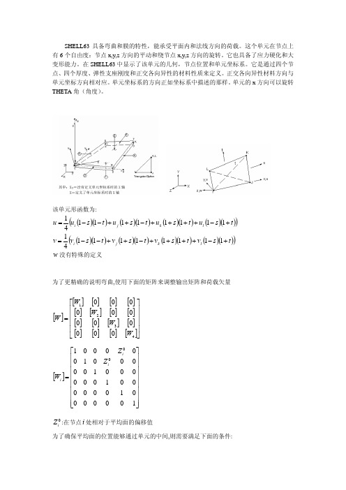
SHELL63具备弯曲和膜的特性,能承受平面内和法线方向的荷载。
这个单元在节点上有6个自由度:节点x,y,z 方向的平动和绕节点x,y,z 方向的旋转。
它也具备了应力硬化和大变形能力。
在SHELL63中显示了该单元的几何,节点位置和单元坐标系。
它是通过四个节点、四个厚度、弹性支座刚度和正交各向异性的材料性质来定义。
正交各向异性材料方向与单元坐标方向相对应。
单元坐标系的方向正如坐标系中描述的那样。
单元的x 方向可以旋转THETA 角(角度)。
该单元形函数为: ()()()()()()()(()t s u t s u t s u t s u u l k j i +−++++−++−−=1111111141) ()()()()()()()(()t s v t s v t s v t s v v l k j i +−++++−++−−=1111111141) w 没有特殊的定义为了更精确的说明弯曲,使用下面的矩阵来调整输出矩阵和荷载矢量[][][][][][][][][][][][][][][][][]⎥⎥⎥⎥⎦⎤⎢⎢⎢⎢⎣⎡=4321000000000000W W W W W []⎥⎥⎥⎥⎥⎥⎥⎥⎦⎤⎢⎢⎢⎢⎢⎢⎢⎢⎣⎡=100000010000001000000100000100000100i i i Z Z W 0i Z :在节点i 处相对于平均面的偏移值为了确保平均面的位置能够通过单元的中间,则需要满足下面的条件:004030201=+++Z Z Z Z对于非匀质材料,可以使用和Takemoto 和Cook 理论相类似的方法(利用shell63)来调整,由于只考虑到单元X 方向上的影响,则可以通过下面的式子将位移和荷载相关联起来.x x x tE T ε=x x y xy xx E E E t M κγ⎟⎟⎠⎞⎜⎜⎝⎛⎟⎟⎠⎞⎜⎜⎝⎛−−=23112x T :单位长度上的力t :厚度x E :在X 方向上的杨氏模量y E :在Y 方向上的杨氏模量x ε:X 方向上的应变x M :单位长度上力矩xy γ:泊松比x κ:X 方向上的曲率通过改进上一个方程,可以得到新的表示非匀质材料的方程 x x y xy xr x E E E t C M κγ⎟⎟⎠⎞⎜⎜⎝⎛⎟⎟⎠⎞⎜⎜⎝⎛−−=23112 2-2r C :弯距乘数因子对于匀质材料来说,其应力可以表示为⎟⎠⎞⎜⎝⎛+=x x top x κt εE σ2 ⎟⎠⎞⎜⎝⎛−=x x bot x κt εE σ2 其中:顶部的X 方向应力 topx σbot x σ:底部的X 方向应力对于非匀质材料来说,其应力可以表示为()x t x top x c E κεσ+=()x b x bot x c E κεσ−=t c :顶部弯曲应力乘数因子b c :底部弯曲应力乘数因子最后输出的力矩(如MX 、MY 、MXY),是通过最后输出的应力来确定的而不是方程2---2表示的。
coupling分为两种:运动耦合和分布耦合

coupling分为两种:运动耦合和分布耦合coupling分为两种:运动耦合和分布耦合;是对接触问题的⼀种简化⽅式,⼀般来讲,分布耦合处的刚度⼩于运动耦合处的刚度;【1】运动耦合:即在此区域的各节点与参考点之间建⽴⼀种运动上的约束关系。
【2】分布耦合:在此区域的各节点与参考点之间建⽴⼀种约束关系,但是对此区域上各节点的运动进⾏了加权处理,使在此区域上受到的合⼒和合⼒距与施加在参考点上的⼒和⼒矩相等效。
换⾔之,分布耦合允许⾯上的各部分之间发⽣相对变形,⽐运动耦合中的⾯更柔软。
31.3.2 Coupling constraintsProducts: Abaqus/Standard Abaqus/Explicit Abaqus/CAEReferences“Surfaces: overview,” Section 2.3.1*COUPLING*KINEMATIC*DISTRIBUTING“Defining coupling constraints,” Section 15.15.4 of the Abaqus/CAE User's ManualOverviewThe surface-based coupling constraint:couples the motion of a collection of nodes on a surface to the motion of a reference node;is of type kinematic when the group of nodes is coupled to the rigid body motion defined by the reference node;is of type distributing when the group of nodes can be constrained to the rigid body motion defined by a reference node in an average sense by allowing control over the transmission of forces through weight factors specified at the coupling nodes;automatically selects the coupling nodes located on a surface lying within a region of influence;can be used with two- or three-dimensional stress/displacement elements; andcan be used in geometrically linear and nonlinear analysis.Surface-based coupling definitionsThe surface-based coupling constraint in Abaqus provides coupling between a reference node and a group of nodes referred to as the “coupling nodes.” This option provides the same functionality as the kinematic coupling constraint and the distributing coupling elements (DCOUP2D, DCOUP3D) in Abaqus/Standard with a surface-based user interface. The coupling nodes are selected automatically by specifying a surface and an optional influence region. The procedure used to define the coupling nodes is discussed below.For a distributing coupling constraint, the distributing weight factors are calculated automatically if the surface is an element-based surface. In such a case the weight factors are based on the tributary area at each coupling node, except for a surface along a shell edge, where the weight factors are based on the tributary edge length. Furthermore, the distributing weight factors can be modified using one of several weighting methods, which allow the forces transferred to the coupling nodes to vary inversely with the radial distance from the reference node.Typical applicationsThe coupling constraint is useful when a group of coupling nodes is constrained to the rigid body motion of a single node. The coupling constraint can be employed effectively in the following applications:To apply loads or boundary conditions to a model. Figure 31.3.2–1 illustrates the use of a kinematic coupling constraint to prescribe a twisting motion to a model without constraining the radial motion.Figure 31.3.2–1 Kinematic coupling constraint.Figure 31.3.2–2 illustrates a distributing coupling constraint used to prescribe a displacement and rotation condition ona boundary where relative motion between the nodes on the boundary is required. In this example a twist is prescribedat the end of the structure that is expected to warp and/or deform within the end surface.Figure 31.3.2–2 Distributing coupling constraint.To distribute loads on a model, where the load distribution can be described with a moment-of-inertia expression.Examples of such cases include the classic bolt-pattern and weld-pattern distribution expressions.To apply dimensionality transitions between continuum and structural elements. For example, a distributing coupling allows flexible coupling between structural and solid elements.To model end conditions. For example, modeling a rigid end plate or modeling plane sections of a solid to remain planar can be done easily with a kinematic coupling definition.To simplify modeling of complex constraints. In a kinematic coupling definition the degrees of freedom that participate in the constraint may be selected individually in a local coordinate system.To model interactions with other constraints, such as connector elements. For example, a hinged part may be modeled more realistically by two distributing coupling definitions, whose reference nodes are connected by a hinge connector element. The load transfer then occurs between two “clouds” of nodes, rather than between two single nodes.“Substructure analysis of a one-piston engine model,” Section 4.1.10 of the Abaqus Example Problems Manual,illustrates this use of connector elements in conjunction with coupling constraints to model a one-piston engine. Defining the coupling constraintDefining a coupling constraint requires the specification of the reference node (also called the constraint control point), the coupling nodes, and the constraint type. The coupling constraint associates the reference node with the coupling nodes. A name must be assigned to the constraint and may be used in postprocessing with Abaqus/CAE. A node number or node set name may be specified for the reference node. If a node set is specified, the node set must contain exactly one node. The reference node for a kinematic coupling constraint has both translational and rotational degrees of freedom. The surface on which the coupling nodes are located can be node-based; element-based; or, in Abaqus/Explicit, a combination of both surface types. You can specify an optional radius of influence that limits the coupling nodes to a specific region on the surface. Details on how coupling nodes are defined by specifying an influence region are discussed below.The constraint type can be either kinematic or distributing, as discussed below.Input File Usage:Use the following options:*COUPLING, CONSTRAINT NAME=name, REF NODE=n,SURFACE=surface*KINEMATIC or*DISTRIBUTINGAbaqus/CAE Usage:Interaction module: Create Constraint: Coupling: Coupling type: Kinematic or DistributingSpecifying a region of influenceBy default, coupling nodes belonging to the entire surface are selected for the coupling definition. You can limit the coupling nodes to lie within a spherical region centered about the reference node by defining a radius of influence.The procedure by which coupling nodes are selected for the constraint definition depends on the surface type:For a node-based surface, all the nodes defined by the surface definition that fall within the influence region areselected for the coupling definitions.For an element-based surface, the surface facets that are either fully or partially inscribed by the influence region are determined. All nodes belonging to these facets, whether or not these nodes fall within the influence region, areselected for the coupling nodes. When the influence radius is less than the distance to the closest coupling node, Abaqus selects all nodes belonging to the closest facet. If the projection of the reference node on the surface falls on an edge or a vertex of multiple facets, all nodes belonging to these facets adjoining the edge or vertex are included in the coupling definition.A distributing coupling constraint must include at least two coupling nodes. If fewer than two coupling nodes are found,Abaqus issues an error message during input file preprocessing.Input File Usage:*COUPLING, CONSTRAINT NAME=name, REF NODE=n,SURFACE=surface, INFLUENCE RADIUS=rAbaqus/CAE Usage:Interaction module: Create Constraint: Coupling: Influence radius: SpecifyKinematic coupling constraintsKinematic coupling constrains the motion of the coupling nodes to the rigid body motion of the reference node. The constraint can be applied to user-specified degrees of freedom at the coupling nodes with respect to the global or a local coordinate system.Kinematic constraints are imposed by eliminating degrees of freedom at the coupling nodes. In Abaqus/Standard once any combination of displacement degrees of freedom at a coupling node is constrained, additional displacement constraints—such as MPCs, boundary conditions, or other kinematic coupling definitions—cannot be applied to any coupling node involved in a kinematic coupling constraint. The same limitation applies for rotational degrees of freedom. This restriction does not apply in Abaqus/Explicit. See “Kinematic constraints: overview,” Section 31.1.1, for more information.Input FileUsage:Use both of the following options to define a kinematic coupling constraint:*COUPLING*KINEMATICfirst dof, last dofFor example, the following coupling constraint is used to constrain degrees of freedom 1, 2, and 6 on surfacesurfA to reference node 1000:*COUPLING, CONSTRAINT NAME=C1, REF NODE=1000, SURFACE=surfA*KINEMATIC1, 26,Abaqus/CAE Usage:Interaction module: Create Constraint: Coupling: Coupling type: Kinematic: toggle on the degrees of freedomTranslational degrees of freedomTranslational degrees of freedom are constrained by eliminating the specified degrees of freedom at the coupling nodes. When all translational degrees of freedom are specified, the coupling nodes follow the rigid body motion of the reference node.Rotational degrees of freedomRotational degrees of freedom are constrained by eliminating the specified degrees of freedom at the coupling nodes. All combinations of selected rotational degrees of freedom result in rotational behavior identical to existing MPC types: Selection of three rotational degrees of freedom along with three displacement degrees of freedom is equivalent to MPC type BEAM.Selection of two rotational degrees of freedom is equivalent to MPC type REVOLUTE in Abaqus/Standard.Selection of one rotational degree of freedom is equivalent to MPC type UNIVERSAL in Abaqus/Standard.In Abaqus/Standard internal nodes are created by the kinematic coupling to enforce the constraints that are equivalent to MPC types REVOLUTE and UNIVERSAL. These nodes have the same degrees of freedom as the additional nodes used in these MPC types and are included in the residual check for nonlinear analysis.Specifying a local coordinate systemThe kinematic coupling constraint can be specified with respect to a local coordinate system instead of the global coordinate system (see “Orientations,” Section 2.2.5). Figure 31.3.2–1 illustrates the use of a local coordinate system to constrain all but the radial translation degrees of freedom of the coupling nodes to the reference node. In this example a local cylindrical coordinate system is defined that has its axis coincident with the structure's axis. The coupling node constraints are then specified in this local coordinate system.Input File*COUPLING, ORIENTATION=localUsage:For example, the following input is used to specify the kinematic coupling constraint shown in Figure31.3.2–1:*ORIENTATION, SYSTEM=CYLINDRICAL, NAME=COUPLEAXIS0.0, -1.0, 0.0, 0.0, 1.0, 0.0*COUPLING, REF NODE=500, SURFACE=Endcap,ORIENTATION=COUPLEAXIS*KINEMATIC2, 3Abaqus/CAE Usage:Interaction module: Create Constraint: Coupling: Edit: select local coordinate systemConstraint direction and finite rotationIn geometrically nonlinear analysis steps the coordinate system in which the constrained degrees of freedom are specified will rotate with the reference node regardless of whether the constrained degrees of freedom are specified in the global coordinate system or in a local coordinate system.Distributing coupling constraintsDistributing coupling constrains the motion of the coupling nodes to the translation and rotation of the reference node. This constraint is enforced in an average sense in a way that enables control of the transmission of loads through weight factors at the coupling nodes. Forces and moments at the reference node are distributed either as a coupling node-force distribution only (default) or as a coupling node-force and moment distribution. The constraint distributes loads such that the resultants of the forces (and moments) at the coupling nodes are equivalent to the forces and moments at the reference node. For cases of more than a few coupling nodes, the distribution of forces/moments is not determined by equilibrium alone, and distributing weight factors are used to define the force distribution.The moment constraint between the rotation degrees of freedom at the reference node and the average rotation of the cloud nodes can be released in one direction in a two-dimensional analysis and one, two, or three directions in a three-dimensional analysis. In a three-dimensional analysis you can specify the moment constraint directions in the global coordinate system or in a local coordinate system. All available translational degrees of freedom at the reference node are always coupled to the average translation of the coupling nodes.In a three-dimensional Abaqus/Standard analysis if all three moment constraints are released by specifying only degrees of freedom 1 through 3, only translation degrees of freedom will be activated on the reference node. If only one or two rotation degrees of freedom have been released, all three rotation degrees of freedom are activated at the reference node. In this case you must ensure that proper constraints have been placed on the unconstrained rotation degrees of freedom to avoid numerical singularities. Most often this is accomplished by using boundary conditions or by attaching the reference node to an element such as a beam or shell that will provide rotational stiffness to the unconstrained rotation degrees of freedom.In Abaqus/Explicit releasing one or more of the moment constraints may lead to significant computational performance degradation. This is also the case when other constraints intersect the cloud of coupling nodes. In these cases, the degradation in performance is particularly noticeable when a large number of such distributed couplings are present in the model or when the size of the constrained “cloud” is large. For that matter, when the modeling conditions mentioned above are encountered, the size of the coupling nodes cloud is limited to 1000. To alleviate the released moment constraint issue,the following modeling technique can be used (also available in Abaqus/Standard): constrain all moments in the distributed coupling and use an appropriate connector element at the reference node (such as REVOLUTE, HINGE, CARDAN or BUSHING) to model released moments at the coupling's reference node. This technique has also the advantage of being able to specify finite compliance such as elasticity, plasticity or damage in the “released” rotational component.Input FileUsage:*DISTRIBUTINGfirst dof , last dof If no degrees of freedom are specified, all available degrees of freedom are coupled. If you specify one or morerotation degrees of freedom but not all available translation degrees of freedom, Abaqus issues a warning message and adds all available translation degrees of freedom to the constraint.For example, the following coupling constraint is used to constrain degrees of freedom 1–5 on the reference node1000 to the average translation and rotation of surface surfA :*COUPLING , CONSTRAINT NAME=C1, REF NODE=1000, SURFACE=surfA *DISTRIBUTING1, 5In this example the moment constraint between the reference node and the coupling nodes will be released in the 6-direction but will be enforced in the 4- and 5-directions. This provides a “revolute-like” rotation connection between the reference node and the coupling nodes (see “General multi-point constraints,” Section 31.2.2).Abaqus/CAE Usage:Interaction module: Create Constraint : Coupling : Coupling type : Distributing : toggle on the rotational degrees of freedom (Abaqus/CAE automatically constrains the translational degrees of freedom)Node-based surfaceUser-defined weight factors are used for node-based surfaces. The cross-sectional areas specified in the surface definition are used as the weight factors (see “Node-based surface definition,” Section 2.3.3).Element-based surfaceFor element-based surfaces the weight factors are calculated by Abaqus. The default weight distribution is based on the tributary surface area at each coupling node, except for a surface along a shell edge where the weight distribution is based on the tributary edge length. The procedure used to calculate the default weight factors is designed to ensure that if a radius of influence is prescribed, the default weight distribution varies smoothly with the influence radius.Calculating the default distributing weight factors The procedure to calculate the distributing weight factors depends on whether or not an influence radius is specified.If no influence radius is specified, the entire surface is used in the coupling definition. In this case all nodes located on the surface are included in the coupling definition and the distributing weight factor at each coupling node is equal to the tributary surface area.If an influence radius is specified, the default distributing weight factors at the coupling nodes are calculated as follows:1. A “participation factor” is calculated for each surface facet. The participation factor is defined below.2. The tributary nodal area (or tributary edge length along a shell edge) at each facet node is computed and ismultiplied by the facet participation factor.3. The coupling node distributing weight factor is computed as the sum of the corresponding facet nodal areas(calculated above) for all joining facets.Calculating the facet participation factorThe participation factor defines the proportion of the facet's area that contributes to the distributing weight factors when an influence radius is specified. The participation factor varies between zero and one.To define the participation factor, the distance of the facet node closest to the reference node, , and the distance of the facet node farthest from the reference node, , are calculated.If , where is the influence radius, all facet nodes lie within the influence region; and a participation factor of one is used.If , none of the facet nodes lie within the influence region; and the participation factor is set to zero.If , the facet is partially inscribed in the influence region; and the facet is assigned a participation factor equal to .If all coupling nodes fall outside the influence radius (i.e., for all facets), Abaqus selects all nodes belonging to the closest facets (as outlined under “Specifying a region of influence”) and uses a participation factor equal to one.Weighting methodsYou can modify the default weight distribution defined above. Various weighting methods are provided that monotonically decrease with radial distance from the reference node. For each case the default weight distribution that is based on the tributary surface area (or tributary edge length along a shell edge) is scaled by the weight factor . If the weighting method is not specified, a uniform weighting method is used in which all weight factors are equal to 1.0.Linearly decreasing weight distributionA linearly decreasing weighting schemewhere is the weight factor at coupling node i, is the coupling node radial distance from the reference node, and is the distance to the furthest coupling node.Input File Usage:*DISTRIBUTING, WEIGHTING METHOD=LINEARAbaqus/CAE Usage:Interaction module: Create Constraint: Coupling: Coupling type: Distributing: Weighting method: LinearQuadratic polynomial weight distributionA quadratic polynomial weight distribution defined byInput File Usage:*DISTRIBUTING, WEIGHTING METHOD=QUADRATICAbaqus/CAE Usage:Interaction module: Create Constraint: Coupling: Coupling type: Distributing: Weighting method: QuadraticMonotonically decreasing weight distributionA monotonically decreasing weight distribution according to the cubic polynomial Input File Usage:*DISTRIBUTING, WEIGHTING METHOD=CUBICAbaqus/CAE Usage:Interaction module: Create Constraint: Coupling: Coupling type: Distributing: Weighting method: CubicSpecifying a local coordinate systemThe distributing coupling constraint can be specified with respect to a local coordinate system instead of the global coordinate system (see “Orientations,” Section 2.2.5). Figure 31.3.2–2 illustrates the use of a local coordinate system to release the moment constraints between the reference node and the coupling nodes in the local 4- and 6-directions, providing a “universal-like” rotation connection. In this example a local rectangular coordinate system is defined that has its local y-axis coincident with the global z-axis. The moment constraint is specified in this local coordinate system.Input FileUsage:*COUPLING, ORIENTATION=localFor example, the following input is used to specify the distributing coupling constraint shown in Figure31.3.2–2:*ORIENTATION, SYSTEM=RECTANGULAR, NAME=COUPLEAXIS0.0, 1.0, 0.0, 0.0, 0.0, 1.0*COUPLING, REF NODE=500, SURFACE=Endcap,ORIENTATION=COUPLEAXIS*DISTRIBUTING1, 35, 5Abaqus/CAE Usage:Interaction module: Create Constraint: Coupling: Edit: select local coordinate systemDefining the surface coupling methodThere are two methods available to couple the motion of the reference node to the average motion of the coupling nodes: the continuum coupling method and the structural coupling method. The continuum coupling method is used by default. Continuum coupling methodThe default continuum coupling method couples the translation and rotation of the reference node to the average translation of the coupling nodes. The constraint distributes the forces and moments at the reference node as a coupling nodes force distribution only. No moments are distributed at the coupling nodes. The force distribution is equivalent to the classic bolt pattern force distribution when the weight factors are interpreted as bolt cross-section areas. The constraint enforces a rigid beam connection between the attachment point and a point located at the weighted center of position of the coupling nodes. For further details, see “Distributing coupling elements,” Section 3.9.8 of the Abaqus Theory Manual.Input File Usage:*DISTRIBUTING , COUPLING=CONTINUUMAbaqus/CAE Usage:Coupling the motion of the reference node to the average motion of the coupling nodes is not supported in Abaqus/CAE.Structural coupling methodThe structural coupling method couples the translation and rotation of the reference node to the translation and the rotation motion of the coupling nodes. The method is particularly suited for bending-like applications of shells when the coupling constraint spans small patches of nodes and the reference node is chosen to be on or very close to the constrained surface. The constraint distributes forces and moments at the reference node as a coupling node-force and moment distribution. For this coupling method to be active, all rotation degrees of freedom at all coupling nodes must be active (as would be the case when the constraint is applied to a shell surface) and the constraints must be specified in all degrees of freedom (default). In addition, for the constraint to be meaningful, the local (or global) z-axis used in the constraint should be such that it is parallel to the average normal direction of the constrained surface.With respect to translations, the constraint enforces a rigid beam connection between the reference node and a moving point that remains at all times in the vicinity of the constrained surface. The location of this moving point is determined by the approximate current curvature of the surface, the current location of the weighted center of position of the coupling nodes (see “Distributing coupling elements,” Section 3.9.8 of the Abaqus Theory Manual), and the z-axis used in the constraint. This choice avoids unrealistic contact interactions if multiple pairs of distributed coupling constraints are used to fasten shell surfaces (see “Breakable bonds,” Section 33.1.9, for more details).With respect to rotations, the constraint is different along different local directions. Along the z-axis (twist direction), the constraint is identical to the one enforced via the continuum coupling method (see “Distributing coupling elements,” Section 3.9.8 of the Abaqus Theory Manual). By contrast, the rotational constraint in the plane perpendicular to the z-axis relates the in-plane reference node rotations to the in-plane rotations of the coupling nodes in the immediate vicinity of the reference node. This choice provides a more realistic (compliant) response when the constrained surface is small and deforms primarily in a bending mode.Input File Usage:*DISTRIBUTING, COUPLING=STRUCTURALAbaqus/CAE Usage:Coupling the motion of the reference node to the average motion of the coupling nodes is not supported in Abaqus/CAE.Moment release and finite rotationIn geometrically nonlinear analysis steps the coordinate system of the degrees of freedom that define the moment releaserotates with the reference node regardless of whether the global coordinate system or a local coordinate system is used. Colinear coupling node arrangementsThe distributing coupling constraint transmits moments at the reference node as a force distribution among the coupling nodes, even if these nodes have rotational degrees of freedom. Thus, when the coupling node arrangement is colinear, the constraint is not capable of transmitting all components of a moment at the reference node. Specifically, the moment component that is parallel to the colinear coupling node arrangement will not be transmitted. When this case arises, a warning message is issued that identifies the axis about which the element will not transmit a moment.LimitationsA distributing coupling constraint cannot be used with axisymmetric elements with asymmetric deformation. Thiselement type is not compatible with the distributing coupling constraint.A distributing coupling definition with a large number of coupling nodes produces a large wavefront inAbaqus/Standard. This may result in significant memory usage and a long solution time to solve the finite element equilibrium equations.A distributing coupling constraint cannot involve more than 46,000 degrees of freedom in Abaqus/Standard, whichimplies an upper limit of 23,000 nodes per constraint for two-dimensional and axisymmetric cases and an upper limit of 15,333 nodes per constraint for three-dimensional cases.。
abaqus coupling约束详解(一)

abaqus coupling约束详解(一)Abaqus Coupling 约束详解1. 背景介绍Abaqus Coupling 是一种在ABAQUS分析中使用的约束技术,用于将多个物理过程耦合在一起,并模拟复杂的多物理场行为。
本文将对Abaqus Coupling约束进行详细解释。
2. 什么是 Coupling 约束约束定义Coupling 约束是一种定义在 ABAQUS 分析中的约束,它将不同的物理过程相互联系起来。
通过约束,可以将结构分析与流体分析、温度分析等不同的物理过程耦合在一起。
Coupling 约束的作用Coupling 约束可以用于模拟多物理场行为,如力学变形、热传导、热机械耦合、电磁-机械耦合等。
它可以将不同物理过程之间的相互作用考虑在内,提供更准确和全面的仿真结果。
3. 如何定义 Coupling 约束Coupling 约束的定义是通过 ABAQUS 中定义辅助场实现的。
辅助场可以是速度场、温度场、压力场等。
下面是一些定义 Coupling 约束的关键步骤:1.定义辅助场:在 ABAQUS 中,首先需要定义辅助场。
辅助场可以通过点、面或体元素来定义,具体根据需要而定。
2.定义耦合:在辅助场定义后,需要在主场和辅助场之间定义耦合。
耦合可以是线性、非线性的。
3.定义边界条件:根据实际问题,定义主场和辅助场的边界条件。
4.定义求解步:在 ABAQUS 中定义求解步,将耦合问题加入到分析中。
5.运行分析:通过 ABAQUS 提供的求解器来运行分析,得到耦合问题的解。
4. Coupling 约束的应用Coupling 约束可以在很多领域中得到应用,如:•结构与流体耦合:模拟风洞试验、流体-结构相互作用等。
•热机械耦合:模拟冲击加载下的结构变形与温度变化。
•电磁-机械耦合:模拟电机的运动和输出功率。
5. 结论Coupling 约束是一种在 ABAQUS 分析中用于模拟多物理场行为的重要技术。
abaqus部分名词定义及解释
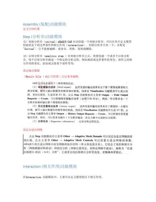
Assembly (装配)功能模块定义空间位置Step (分析步)功能模块(l)初始分析步(initial)ABAQUS/CAE自动创建一个初始分析步,可以在其中定义模型初始状态下的边界条件和相互作用(interaction)。
初始分析步只有一个,名称是"Initial",它不能被编辑、重命名、替换、复制或删除。
(2)后续分析步(analysis step )在初始分析步之后,需要创建一个或多个后续分析步,每个后续分析步描述一个特定的分析过程,例如载荷或边界条件的变化、部件之间相互作用的变化、添加或去除某个部件等等:设定输出数据(Result file )fil可供第三方记事本编辑。
设定自适应网格Interaction (相互作用)功能模块在Interaction 功能模块中,主要可以定义模型的以下相互作用。
1.Interaction 定义模型的各部分之间或模型与外部环境之间的力学或热相互作用,例如接触、弹性地基、热辐射等。
2.Constraint 定义模型各部分之间的约束关系。
3.Connector 定义模型中的两点之间或模型与地面之间的连接单元( connector),用来模拟固定连接、钱接、恒定速度连接、止动装置、内摩擦、失效条件和锁定装置等。
4.Special →Inertia 定义惯量(包括点质量/惯量、非结构质量和热容)。
5.Special →Crack 定义裂纹。
6.Special →Springs/Dashpots定义模型中的两点之间或模型与地面之间的弹簧和阻尼器。
7.主菜单Tools 常用的菜单项包括Set (集合)、Surface (面)和AlE\plitude (幅值)等。
说明:接触即使两实体之间或一个装配件的两个区域之间在空间位置上是互相接触的,ABAQUS/CAE 也不会自动认为它们之间存在着接触关系,需要使用interaction模块中的主菜单Interacton 来定义这种接触关系。
- 1、下载文档前请自行甄别文档内容的完整性,平台不提供额外的编辑、内容补充、找答案等附加服务。
- 2、"仅部分预览"的文档,不可在线预览部分如存在完整性等问题,可反馈申请退款(可完整预览的文档不适用该条件!)。
- 3、如文档侵犯您的权益,请联系客服反馈,我们会尽快为您处理(人工客服工作时间:9:00-18:30)。
Abaqus Analysis User's Manual31.3.3 Shell-to-solid couplingProducts: Abaqus/Standard Abaqus/Explicit Abaqus/CAEReferencesOverviewSurface-based shell-to-solid coupling:∙allows for a transition from shell element modeling to solid element modeling;∙is most useful when local modeling should use a full three-dimensional analysis but other parts of the structure can be modeled as shells;∙uses a set of internally defined distributing coupling constraints to couple the motion of a “line” of nodes along the edge of a shell model to the motion of a set of nodes on a solid surface;∙automatically selects the coupling nodes located on a solid surface lying within a region of influence;∙can be used with three-dimensional stress/displacement shell and solid (continuum) elements;∙does not require any alignment between the solid and shell element meshes; and∙can be used in geometrically linear and nonlinear analysis.Shell-to-solid couplingShell-to-solid coupling in Abaqus is a surface-based technique for couplingpinched cylinder problem,”Section 2.3.2 of the Abaqus Benchmarks Manual. Shell-to-solid coupling is intended to be used for mesh refinement studies where local modeling requires a relatively fine through-the-thickness solid mesh coupled to the edge of a shell mesh, as shown in Figure 31.3.3–2. In such a case Abaqus will assemble constraints that couple the displacement and rotation of each shell node to the average displacement and rotation of the solid surface in the vicinity of the shell node.Figure 31.3.3–1 Typical examples of shell-to-solid coupling.Figure 31.3.3–2 Shell-to-solid interface.As shown in Figure 31.3.3–2, the coupling occurs along a shell-to-solid interface defined by two user-specified surfaces: an edge-based shell surface and an element- or node-based solid surface (see “Surfaces:overview,”Section 2.3.1). The shell surface (Figure 31.3.3–3) is referred to as the “shell edge.”Figure 31.3.3–3 Shell and solid surfaces.The shell element edges that define the edge-based shell surface are referred to as “edge facets.” The edge facets are either linear or parabolic segments depending if the underlying shell elements are linear or quadratic.The shell-to-solid coupling is enforced by the automatic creation of an internal set of distributing coupling constraints (see “Coupling constraints,”Section 31.3.2) between nodes on the shell edge and nodes on the solid surface.Abaqus uses default or user-defined distance and tolerance parameters (discussed below) to determine which nodes on the shell edge will be coupled to which nodes on the solid surface. For each shell node involved in the coupling, a distinct internal distributing coupling constraint is created with the shell node acting as the reference node and the associated solid nodes acting as the coupling nodes. Each internal constraint distributes the forces and moments acting at its shell node as forces acting on the related set of coupling surface nodes in a self-equilibrating manner. The resulting line of constraints enforces the shell-to-solid coupling.Defining shell-to-solid couplingDefining a shell-to-solid coupling constraint requires the specification of a constraint name, an edge-based shell surface, and an element- or node-based solid surface.Input File Usage: *SHELL TO SOLID COUPLING, CONSTRAINTNAME=nameshell_surface, solid_surfaceAbaqus/CAE Usage: I nteraction module: Create Constraint: Shell-to-solidcouplingAbaqus automatically determines which nodes on the two surfaces participate in the coupling and creates appropriate internal distributed coupling constraints. You can also control which nodes on the two surfaces participate in the coupling by specifying a position tolerance and/or influence distance as described below.The resulting coupling constraint definitions are printed to the data file when model definition data are requested (see “Controlling the amount of analysis input file processor information written to the data file” in “Output,”Section4.1.1). Abaqus will also create an internal node set that contains all the solid nodes included in the coupling; the node set can be visualized usingthe Visualization module of Abaqus/CAE. The name of the internal node set is the name assigned to the coupling constraint.Controlling the shell nodes included in the couplingA position tolerance determines the absolute distance from the solid surface within which all shell nodes to be included in the coupling must lie. Shell nodes that lie outside this tolerance are not coupled to the solid surface.When using an element-based solid surface, the defined distance between a shell node and the solid surface is the projected distance measured along a line extending from the shell node to the closest point on the solid surface (which may be on the edge of the solid surface). The default position tolerance when using an element-based solid surface is 5% of the length of a typical facet on the shell edge.For a node-based solid surface the defined distance of a shell node to the surface is the distance to the closest node on the solid surface. The default position tolerance when using a node-based solid surface is based on the average distance between nodes on the solid surface.You can specify a nondefault position tolerance for element- or node-based solid surfaces..Input File Usage: *SHELL TO SOLID COUPLING, POSITIONTOLERANCE=distanceAbaqus/CAE Usage: I nteraction module: Create Constraint: Shell-to-solidcoupling: select the surfaces: choose Specifydistance for the Position ToleranceControlling the solid nodes included in the couplingA geometric tolerance, which is referred to as the influence distance, is defined for each edge facet. For a given node or element facet on the solid surface to be included in the coupling constraint, its perpendicular distance from at least one edge facet must be less than or equal to the influence distance defined for that edge facet. The default influence distance for an edge facet is half the thickness of the underlying shell element. The default automatically accounts for any offset or nodal thickness included with the shell element's cross-section definition. You can specify a nondefault influence distance.Input File Usage: *SHELL TO SOLID COUPLING, INFLUENCEDISTANCE=distanceAbaqus/CAE Usage: I nteraction module: Create Constraint: Shell-to-solidcoupling: select the surfaces: choose Specify value forthe Influence DistanceA user-defined influence distance is optional in all cases except when an edge facet involved in the coupling is associated with a general arbitrary elastic shell section definition in which you specified the general stiffness. In this case sincethe shell thickness is not defined directly, you must supply an influence distance.Computation of the internal coupling constraintsThis section outlines the basic procedure used by Abaqus to compute the internal shell-to-solid coupling constraints.A single distinct internal distributing coupling constraint is created for each shell node that lies within the position tolerance from the solid surface. Internal coupling constraints are not created for shell nodes that lie outside this tolerance. The shell node acts as the reference node, and a set of nodes on the solid surface act as the coupling nodes. Abaqus finds the coupling nodes on the solid surface and computes the weight factors for the internal constraints by considering each shell edge facet separately. The following procedure is carried out for each edge facet:1. Abaqus finds all nodes on the solid element surface that lie within theregion of influence (discussed below) of the current edge facet. Thesenodes are included in the coupling constraint.2. Abaqus then computes a set of weight factors for the solid nodes. Aweight factor is a measure of both the tributary area of the solid nodecontained within the region of influence and the relative position of thesolid node with respect to each shell node. The tributary areas fornode-based surfaces are the cross-sectional areas that you specifiedwhen you defined the surface. For element-based surfaces the tributary areas are calculated by Abaqus. The sum of all the weight factors ineach coupling constraint is a measure of the total tributary area of thesolid surface that is contained within the region of influence.3. The above procedure is carried out for all the shell edge facetscontained within the shell surface. If a shell node belongs to more than one edge facet, all the coupling nodes and weight factors are combined into a single distributing constraint definition. The resulting line ofconstraints along the shell edge enforces the shell-to-solid coupling. There are two situations in which a shell node might satisfy the position tolerance but no coupling constraint is defined. If a shell node lies within the position tolerance but is not connected by an edge facet to at least one other shell node that also satisfies the tolerance, a coupling constraint is not created for this shell node. In this case it may be necessary to increase the position tolerance. Alternatively, if nonzero weight factors are not computed for at least two solid nodes associated with the shell node, a coupling constraint is not created for this shell node. The most likely cause for zero weight factors is that the influence distance is too small. In the case of a node-based surface, zeroweights might also arise if the default cross-sectional area is used. Forshell-to-solid coupling the default area is zero.The region of influence for an edge facetThe region of influence of an edge facet is defined by a cylindrical volume whose centerline is the edge facet and whose radius is the edge facet's influence distance. The ends of the cylindrical volume are defined by two bounding planes whose normals are the shell tangents at the two ends of the edge facet (see Figure 31.3.3–4).Figure 31.3.3–4 Regions of influence for an edge facet.In this example a region of influence is constructed for shell edge 2–3. For a node-based solid surface only the nodes that lie within or on the boundary of the region of influence are assigned to the current edge facet and included in the coupling definition. For an element-based solid surface each solid facet node is associated with part of the facet surface. If the part of the facet assigned to a given solid node falls within the region of influence, that node is included in the coupling definition.Using the normal on an element-based solid surface to restrict solid nodes that are used in the couplingIn the case of an element-based solid surface Abaqus will compare the normal of each solid facet within the region of influence to the normal of the solid surface closest to the centerline of the cylindrical volume (see Figure 31.3.3–4).In general, if the normal of a surface facet is not within 20° of the normal at the centerline, the nodes on the solid surface facet are not included in the coupling definition. For the case illustrated in Figure 31.3.3–4 this check would prevent nodes on the top and bottom surface of the solid mesh from being coupled to the shell nodes even if the influence distance was arbitrarily large and the solid surface definition included all sides of the solid geometry. This check is not used if the centerline is on or near a feature edge of the solid mesh where the normal is not well defined (see the discussion about shell offsets below). Comments, restrictions, and modeling recommendations forshell-to-solid coupling∙The shell-to-solid coupling formulation assumes that the interface surface between the shell and solid elements is normal to the shell.Therefore, while the solid surface can be curved in a direction tangentto the shell edge, it should be straight in the direction along the shellnormals. This is an assumption on the geometry of the surfaces, not on the mesh. It is not necessary for the nodes on the solid surface to lineup with each other or to line up with the shell nodes.∙The shell-to-solid coupling capability is designed for analyses where the solid mesh is fine with respect to the shell thickness. It is recommended that at least two solid elements be included through the thickness at ashell-to-solid interface. Along the shell-to-solid interface the length of a shell edge facet should in general be of the same order as thecharacteristic surface dimension of a solid element facet.∙An assumption used in the design of the shell-to-solid coupling algorithms is that the weight factors are based upon accurate nodaltributary areas, such as those automatically computed by Abaqus when an element-based surface is used. Therefore, it is generallyrecommended that an element-based solid surface be used instead of a node-based solid surface. However, in cases where the shell and solid meshes align with each other, it is sometimes advantageous to use anode-based solid surface especially when a homogenous solution isexpected.∙Figure 31.3.3–5 illustrates some recommended modeling practices for shell-to-solid coupling. If the shell reference surface is not offset, theshell edge should be centrally located with respect to the thicknessdirection of the solid (Figure 31.3.3–5(a)). The solid surface shouldinclude only the portion needed for the coupling (the shaded regionshown in Figure 31.3.3–5(a)).Figure 31.3.3–5 Modeling recommendations for the shell-to-solidinterface.∙The shell-to-solid interface can be defined around geometric feature angles (corners), (Figure 31.3.3–5(b)). However, it is recommended that the feature angles satisfy 60° < < 300°. In addition, as illustrated in Figure 31.3.3–5(b), at least two shell element edges should beincluded between each feature angle.∙If an offset is defined for the shell section and the reference shell edge is placed at or near a feature edge on the solid surface (Figure31.3.3–6), the solid surface should include only the side of the solid thatyou want to be included in the coupling definition.Figure 31.3.3–6 Modeling recommendations for the shell-to-solidinterface with a shell offset.For example, if the top of the solid in Figure 31.3.3–6 is included in the surface definition, Abaqus includes nodes on the top of the surface in the coupling constraint, which is not what you intended. You intended only that the shell be coupled to the shaded region of the solid in Figure 31.3.3–6. Therefore, the solid surface definition should include only this region.∙Care must be taken in interpreting the local stress and strain fields in the immediate vicinity of the shell-to-solid interface. This is especially true if the shell-to-solid interface includes corners or edges. Theinterface should be placed at least a distance more than the shellthickness away from the region in the solid mesh where the stress and strain fields are of interest.∙The shell-to-solid interface should be located in a region of the model where shell theory is a valid modeling approximation.∙Corners or kinks may exist in models made of shell elements. At such corners or kinks the shell elements only approximate the distribution of the material away from the midsurface of the shell. While the globalmoments and forces between the shell and solid models are transferred correctly, the local stress and displacement fields in the region of the shell-to-solid interface may be inaccurate.∙Only displacement degrees of freedom in the solid elements and displacement and rotation degrees of freedom in the shell elements are coupled in shell-to-solid coupling. Shell-to-solid coupling does notcouple other degrees of freedom such as temperature, pressure, etc.Shell-to-solid coupling can be used to couple three-dimensional shells to all three-dimensional continuum elements except cylindrical elements(“Cylindrical solid element library,”Section 25.1.5).Abaqus Analysis User's Manual。