Evaluating the Evans Function Order Reduction in Numerical Methods
7097044-Fractional-Calculus

1.2 Historical Survey Most authors on this topic will cite a particular date as the birthday of so called 'Fractional Calculus'. In a letter dated September 30th, 1695 L’Hospital wrote to Leibniz asking him about a particular notation he had used in his publications for the nth-derivative of the Dn x linear function f(x) = x, . L’Hospital posed the question to Leibniz, Dx n what would the result be if n = 1/ 2. Leibniz's response: "An apparent paradox, from which one day useful consequences will be drawn." In these words fractional calculus was born. [7]
Chapter 1
Definition and Applications
3
Fractional Calculus History
value x, verifiable by infinite series expansion, or more practically, by calculator. Now, in the same way consider the integral and derivative. Although they are indeed concepts of a higher complexity by nature, it is still fairly easy to physically represent their meaning. Once mastered, the idea of completing numerous of these operations, integrations or differentiations follows naturally. Given the satisfaction of a very few restrictions (e.g. function continuity) completing n integrations can become as methodical as multiplication. [7] But the curious mind can not be restrained from asking the question what if n were not restricted to an integer value? Again, at first glance, the physical meaning can become convoluted (pun intended), but as this report will show, fractional calculus flows quite naturally from our traditional definitions. And just as fractional exponents such as the square root may find their way into innumerable equations and applications, it will become apparent that integrations of order 1/ 2 and beyond can find practical use in many modern problems. [7]
Part1MonetaryPolicy,Inflation,andtheBusinessCycle
14.461Advanced Macroeconomics I(1st half)Jordi GalíMITFall2005Part1:Monetary Policy,Inflation,and the Business Cycle The lectures will provide an overview of the recent literature on dynamic optimizing models with nominal rigidities and their implications for the design of monetary policy. Lecture notes will be handed out during the course.A list of topics to be be covered and reading list with some of the key articles is provided below.Motivation and EvidenceBeyond RBC Theory.Long Run Evidence.Reduced Form Evidence.The Effects of Monetary Policy Shocks.Walsh,Carl E.(2003):Monetary Theory and Policy,Second Edition,MIT Press,chapter1.McCandless,George T.,Warren Weber(1995):“Some Monetary Facts,”Federal Reserve Bank of Minneapolis,Quartely ReviewBarro,Robert(1998):The Determinants of Economic Growth,MIT Press,chapter3. (NBER WP#5698)Bruno,Michael,and William Easterly(1998):“Inflation Crises and Long Run Growth,”Journal of Monetary Economics,vol.41,no.1,3-26Cooley,Thomas F.and Gary D.Hansen(1995):“Money and the Business Cycle,”in in T. Cooley ed.:Frontiers of Business Cycle Research(Princeton University Press),section7.2.Stock,James,and Mark W.Watson(2000):“Business Cycle Fluctuations in U.S. Macroeconomic Time Series,”in J.B.Taylor and M.Woodford eds.,Handbook of Macroeconomics,volume1A.(also NBER WP6528))Romer,Christina,and David Romer(1989):“Does Monetary Policy Matter?A New Test in the Spirit of Friedman and Schwartz,”NBER Macroeconomics Annual,4,121-170.Christiano,Lawrence J.,Martin Eichenbaum,and Charles L.Evans(1998):“Monetary Policy Shocks:What Have We Learned and to What End?,”in J.B.Taylor and M.Woodford eds.,Handbook of Macroeconomics,volume1A,65-148.(also NBER WP6400).Peersman,Gert and Frank Smets(2003):“The Monetary Transmission Mechanism in the Euro Area:More Evidence from VAR Analysis,”in Angeloni et al.(eds.)Monetary Policy Transmission in the Euro Area,Cambridge University Press,(also ECB WP no.91).Galí,Jordi(1992):”How Well Does the IS-LM Model Fit Postwar U.S.Data?,”Quarterly Journal of Economics709-738.Bernanke,Ben S.,and Ilian Mihov(1997):“Measuring Monetary Policy,”Quarterly Journal of Economics,vol.CXIII,no.3,869-902.Eichenbaum,Martin and Charles E.Evans(1995):“Some Empirical Evidence on the Effects of Shocks to Monetary Policy on Exchange Rates,”Quarterly Journal of Economics110,no.4,975-1010.Bils,Mark and Peter J.Klenow(2004):“Some Evidence on the Importance of Sticky Prices,”Journal of Political Economy,vol112(5),947-985.Dhyne,Emmanuel et al.(2005):“Price Setting in the Euro Area:Some Stylised Facts from Individual Consumer Price Data,”mimeo.Alvarez,Luis et al.(2005):“Sticky Prices in the Euro Area:Evidence from Micro-Data,”mimeo.A Simple Framework for Monetary Policy AnalysisHouseholds.Firms.Marginal costs and markups.Elements of equilibrium.Money demand. Capital accumulation.Walsh,Carl E.(2003):Monetary Theory and Policy,Second Edition,MIT Press,chapter2 (also related:chapter3)Woodford,Michael(2003):Interest and Prices:Foundations of a Theory of Monetary Policy,Princeton University Press,chapter1.Flexible PricesThe classical monetary model.Optimal price setting.Neutrality.Monetary policy rules and price level determination.Sources of non-neutrality.Optimal monetary policy. Hyperinflations.Walsh,Carl E.(2003):Monetary Theory and Policy,Second Edition,MIT Press,chapter2.Woodford,Michael(2003):Interest and Prices:Foundations of a Theory of Monetary Policy,Princeton University Press,chapter2.Cooley,Thomas F.and Gary D.Hansen(1995):“Money and the Business Cycle,”in in T. Cooley ed.:Frontiers of Business Cycle Research(Princeton University Press).Cooley,Thomas F.and Gary D.Hansen(1989):“Inflation Tax in a Real Business Cycle Model,”American Economic Review79,733-748.King,Robert G.,and Mark Watson(1996):“Money,Prices,Interest Rates,and the Business Cycle,”Review of Economics and Statistics,vol78,no1,35-53.Chari,V.V.,and Patrick J.Kehoe(1999):“Optimal Fiscal and Monetary Policy,”in in J.B. Taylor and M.Woodford eds.,Handbook of Macroeconomics,volume1C,1671-1745.Correia,Isabel,and Pedro Teles(1999):“The Optimal Inflation Tax,”Review of Economic Dynamics,vol.2,no.2325-346.A Baseline Sticky Price ModelThe Calvo model.The new Keynesian Phillips curve.The output gap and the natural rate of interest.The effects of monetary policy shocks.Evidence on inflation dynamics.Alternative time-dependent models:convex price adjustment costs,the Taylor model,the truncated Calvo model.State-dependent models.Walsh,Carl E.(2003):Monetary Theory and Policy,Second Edition,MIT Press,chapter5.Woodford,Michael(2003):Interest and Prices:Foundations of a Theory of MonetaryPolicy,Princeton University Press,chapter4.Calvo,Guillermo(1983):“Staggered Prices in a Utility Maximizing Framework,”Journal of Monetary Economics,12,383-398.Yun,Tack(1996):“Nominal Price Rigidity,Money Supply Endogeneity,and Business Cycles,”Journal of Monetary Economics37,345-370.King,Robert G.,and Alexander L.Wolman(1996):“Inflation Targeting in a St.Louis Model of the21st Century,”Federal Reserve Bank of St.Louis Review,vol.78,no.3.(NBER WP#5507).Fuhrer,Jeffrey C.and George R.Moore(1995):“Inflation Persistence”,Quarterly Journal of Economics,Vol.110,February,pp127-159.Galí,Jordi and Mark Gertler(1998):“Inflation Dynamics:A Structural Econometric Analysis,”Journal of Monetary Economics,vol44,no.2,195-222.Sbordone,Argia(2002):“Prices and Unit Labor Costs:A New Test of Price Stickiness,”Journal of Monetary Economics,vol.49,no.2,265-292.Galí,Jordi,Mark Gertler,David López-Salido(2001):“European Inflation Dynamics,”European Economic Review vol.45,no.7,1237-1270.Galí,Jordi,Mark Gertler,David López-Salido(2005):“Robustness of the Estimates of the Hybrid New Keynesian Phillips Curve,”Journal of Monetary Economics,forthcoming.Eichenbaum,Martin and Jonas D.M.Fisher(2004):“Evaluating the Calvo Model of Sticky Prices,”NBER WP10617.Mankiw,N.Gregory and Ricardo Reis(2002):“Sticky Information vs.Sticky Prices:A Proposal to Replace the New Keynesian Phillips Curve,”Quartely Journal of Economics,vol. CXVII,issue4,1295-1328.Rotemberg,Julio(1996):“Prices,Output,and Hours:An Empirical Analysis Based on a Sticky Price Model,”Journal of Monetary Economics37,505-533.Chari,V.V.,Patrick J.Kehoe,Ellen R.McGrattan(2000):“Sticky Price Models of the Business Cycle:Can the Contract Multiplier Solve the Persistence Problem?,”Econometrica, vol.68,no.5,1151-1180.Wolman,Alexander(1999):“Sticky Prices,Marginal Cost,and the Behavior of Inflation,”Economic Quarterly,vol85,no.4,29-48.Dotsey,Michael,Robert G.King,and Alexander L.Wolman(1999):“State Dependent Pricing and the General Equilibrium Dynamics of Money and Output,”Quarterly Journal of Economics,vol.CXIV,issue2,655-690.Dotsey,Michael,and Robert G.King(2005):“Implications of State Dependent Pricing for Dynamic Macroeconomic Models,”Journal of Monetary Economics,52,213-242.Golosov,Mikhail,Robert E.Lucas(2005):“Menu Costs and Phillips Curves”mimeo.Gertler,Mark and John Leahy(2005):“A Phillips Curve with an Ss Foundation,”mimeo.Monetary Policy Design in the Baseline ModelA benchmark case.Optimal monetary policy and its implementation.The Taylor Principle. Simple Monetary Policy Rules.Second order approximation to welfare losses.Evidence on Monetary Policy rules.The effects of technology shocks:theory and evidence.Galí,Jordi(2003):“New Perspectives on Monetary Policy,Inflation,and the BusinessCycle,”in Advances in Economics and Econometrics,volume III,edited by M.Dewatripont, L.Hansen,and S.Turnovsky,Cambridge University Press(also available as NBER WP#8767).Woodford,Michael(2003):Interest and Prices:Foundations of a Theory of Monetary Policy,Princeton University Press,chapter6.Yun,Tack(2005):“Optimal Monetary Policy with Relative Price Distortions”American Economic Review,vol.95,no.1,89-109Blanchard,Olivier and Charles Kahn(1980),“The Solution of Linear Difference Models under Rational Expectations”,Econometrica,48,1305-1311Bullard,James,and Kaushik Mitra(2002):“Learning About Monetary Policy Rules,”Journal of Monetary Economics,vol.49,no.6,1105-1130.Woodford,Michael(2001):“The Taylor Rule and Optimal Monetary Policy,”American Economic Review91(2):232-237(2001).Rotemberg,Julio and Michael Woodford(1999):“Interest Rate Rules in an Estimated Sticky Price Model,”in J.B.Taylor ed.,Monetary Policy Rules,University of Chicago Press.Benhabib,Jess,Stephanie Schmitt-Grohe,and Martin Uribe(2001):“The Perils of Taylor Rules,”Journal of Economic Theory96,40-69.Levin,Andrew,Volker Wieland,and John C.Williams(2003):“The Performance of Forecast-Based Monetary Policy Rules under Model Uncertainty,”American Economic Review,vol.93,no.3,622-645.Clarida,Richard,Jordi Galí,and Mark Gertler(2000):“Monetary Policy Rules and Macroeconomic Stability:Evidence and Some Theory,”Quarterly Journal of Economics,vol. 115,issue1,147-180.Taylor,John B.(1998):“An Historical Analysis of Monetary Policy Rules,”in J.B.Taylor ed.,Monetary Policy Rules,University of Chicago Press.Orphanides,Athanasios(2003):“The Quest for Prosperity Without Inflation,”Journal of Monetary Economics50,633-663Galí,Jordi(1999):“Technology,Employment,and the Business Cycle:Do Technology Shocks Explain Aggregate Fluctuations?,”American Economic Review,vol.89,no.1,249-271.Basu,Susanto,John Fernald,and Miles Kimball(2004):“Are Technology Improvements Contractionary?,”American Economic Review,forthcoming(also NBER WP#10592).Francis,Neville,and Valerie Ramey(2005):“Is the Technology-Driven Real Business Cycle Hypothesis Dead?Shocks and Aggregate FLuctuations Revisited,”Journal of Monetary Economics,forthcoming.Galí,Jordi and Pau Rabanal(2004):“Technology Shocks and Aggregate Fluctuations: How Well Does the RBC Model Fit Postwar U.S.Data?,”NBER Macroeconomics Annual 2004,225-288.(also as NBER WP#10636).Christiano,Lawrence,Martin Eichenbaum,and Robert Vigfusson(2003):“What happens after a Technology Shock?,”NBER WP#9819.Galí,Jordi,J.David López-Salido,and Javier Vallés(2003):“Technology Shocks and Monetary Policy:Assessing the Fed’s Performance,”Journal of Monetary Economics,vol.50, no.4.,723-743.Extensions of the Baseline Model and their Implications for Monetary PolicyCost-push shocks.Nominal wage rigidities.Monetary frictions.Inflation inertia.Real wage rigidities.Steady state distortions.Estimated medium-scale models.Giannoni,Marc P.,and Michael Woodford(2003):“Optimal Inflation Targeting Rules,”in B.Bernanke and M.Woodford,eds.The Inflation Targeting Debate,Chicago,Chicago University Press.(also NBER WP#9939).Woodford,Michael(2003):Interest and Prices:Foundations of a Theory of Monetary Policy,Princeton University Press,chapters6-8.Clarida,Richard,Jordi Galí,and Mark Gertler(1999):“The Science of Monetary Policy:A New Keynesian Perspective,”Journal of Economic Literature,vol.37,no.4,1661-1707.Erceg,Christopher J.,Dale W.Henderson,and Andrew T.Levin(2000):“Optimal Monetary Policy with Staggered Wage and Price Contracts,”Journal of Monetary Economics vol.46,no.2,281-314.Huang,Kevin X.D.,and Zheng Liu.(2002):“Staggered Price-setting,staggeredwage-setting and business cycle persistence,”Journal of Monetary Economics,vo.49,405-433.Woodford,Michael(2003):“Optimal Interest Rate Smoothing,”Review of Economic Studies,vol.70,no.4,861-886.Steinsson,Jón(2003):“Optimal Monetary Policy in an Economy with Inflation Persistence,”Journal of Monetary Economics,vol.50,no.7.Blanchard,Olivier J.and Jordi Galí(2005):“Real Wage Rigidities and the Nw Keynesian Model”mimeo.Benigno,Pierpaolo,and Michael Woodford(2005):“Inflation Stabilization and Welfare: the Case of a Distorted Steady State”Journal of the European Economic Association, forthcoming.Khan,Aubhik,Robert G.King and Alexander L.Wolman(2003):“Optimal Monetary Policy,”Review of Economic Studies,825-860.Christiano,Lawrence J.,Martin Eichenbaum,and Charles L.Evans(2001):“Nominal Rigidities and the Dynamic Effects of a Shock to Monetary Policy,”Journal of Political EconomySmets,Frank,and Raf Wouters(2003):“An Estimated Dynamic Stochastic General Equilibrium Model of the Euro Area,”Journal of the European Economic Association,vol1, no.5,1123-1175.Monetary Policy in the Open EconomyEmpirical issues.Two country models.Small Open Economy.Monetary Unions.Local Currency Pricing.Benigno,Gianluca,and Benigno,Pierpaolo(2003):“Price Stability in Open Economies,”Review of Economic Studies,vol.70,no.4,743-764.Galí,Jordi,and Tommaso Monacelli(2005):“Monetary Policy and Exchange Rate Volatility in a Small Open Economy,”Review of Economic Studies,vol.72,issue3,2005,707-734.Clarida,Richard,Jordi Galí,and Mark Gertler(2002):“A Simple Framework for International Monetary Policy Analysis,”Journal of Monetary Economics,vol.49,no.5, 879-904.Benigno,Pierpaolo(2004):“Optimal Monetary Policy in a Currency Area,”Journal of International Economics,vol.63,issue2,293-320.Monetary and Fiscal Policy InteractionsFiscal policy rules and equilibrium determination.Distortionary taxes and optimal policy. Non-Ricardian economies and the effects ernment spending.Optimal monetary and fiscal policy in currency unions.Leeper,Eric(1991):“Equilibria under Active and Passive Monetary Policies,”Journal of Monetary Economic s27,129-147.Sims,Christopher A.(1994):“A Simple Model for the Determination of the Price Level and the Interaction of Monetary and Fiscal Policy,”Economic Theory,vol.4,381-399.Woodford,Michael(1996):“Control of the Public Debt:A Requirement for Price Stability,”NBER WP#5684.Davig,Troy and Eric Leeper(2005):“Fluctuating Macro Policies and the Fiscal Theory,”mimeo.Schmitt-Grohé,Stephanie,and Martin Uribe(2004):“Optimal Fiscal and Monetary Policy under Sticky Prices,”Journal of Economic Theory114,198-230Schmitt-Grohé,Stephanie,and Martin Uribe(2003):“Optimal Simple and Implementable Monetary and Fiscal Rules,”NBER WP#10253.Blanchard,Olivier and Roberto Perotti(2002),“An Empirical Characterization of the Dynamic Effects of Changes in Government Spending and Taxes on Output,”Quarterly Journal of Economics,vol CXVII,issue4,1329-1368.Fatás,Antonio and Ilian Mihov(2001),“The Effects of Fiscal Policy on Consumption and Employment:Theory and Evidence,”INSEAD,mimeo.Galí,Jordi,J.David López-Salido and Javier Vallés(2005):“Understanding the Effects of Government Spending on Consumption,”mimeo.Galí,Jordi,and Tommaso Monacelli(2005):“Optimal Monetary and Fiscal Policy in a Currency Union:A New Keynesian Perspective,”miemo.。
牛顿法Matlab程序
1
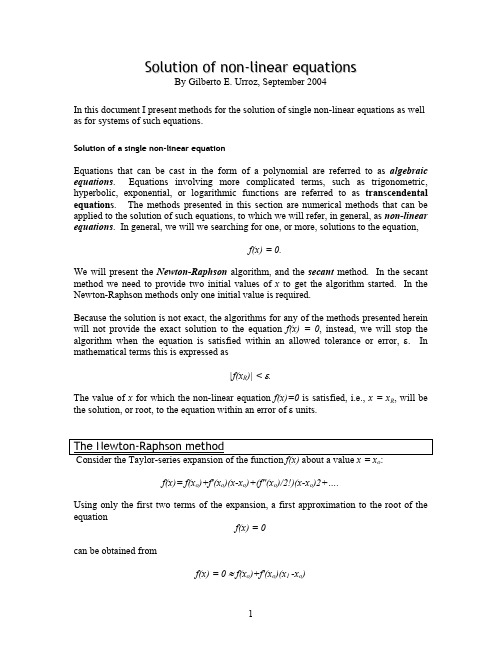
Such approximation is given by, x1 = xo - f(xo)/f'(xo). The Newton-Raphson method consists in obtaining improved values of the approximate root through the recurrent application of equation above. For example, the second and third approximations to that root will be given by and respectively. This iterative procedure can be generalized by writing the following equation, where i represents the iteration number: xi+1 = xi - f(xi)/f'(xi). After each iteration the program should check to see if the convergence condition, namely, |f(x i+1)|<ε, is satisfied. The figure below illustrates the way in which the solution is found by using the NewtonRaphson method. Notice that the equation f(x) = 0 ≈ f(xo)+f'(xo)(x1 -xo) represents a straight line tangent to the curve y = f(x) at x = xo. This line intersects the x-axis (i.e., y = f(x) = 0) at the point x1 as given by x1 = xo - f(xo)/f'(xo). At that point we can construct another straight line tangent to y = f(x) whose intersection with the x-axis is the new approximation to the root of f(x) = 0, namely, x = x2. Proceeding with the iteration we can see that the intersection of consecutive tangent lines with the x-axis approaches the actual root relatively fast. x2 = x1 - f(x1)/f'(x1), x3= x2 - f(x2)/f'(x2),
VALIDATION OF THE SWAT MODEL ON A LARGE RWER BASIN WITH POINT AND NONPOINT SOURCES

1Paper No. 00044 of the Journal of the American Water Resources Association. Discussions are open until June 1, 2002. 2Respectively, Post Doctoral Research Scientist, Blackland Research Center, 720 East Blackland Road, Temple, Texas 76502-9622; Hydraulic Engineer, USDA/ARS, 808 East Blackland Road, Temple, Texas 76502; Research Scientist, Blackland Research Center, 720 East Blackland Road, Temple, Texas 76502-9622; Professor and Resident Director, Blackland Research Center, 720 East Blackland Road, Temple, Texas 76502-9622; Associate Professor and Director of Spatial Sciences Lab, Blackland Research Center, 700 East University Drive, Suite
classified water bodies, 147 have been listed on the
1998 303(d) list. One of these projects is in the Bosque
River Watershed in North Central Texas, where
教育教研论文常用参考书目
参考书目陈琳,2001,小学开设英语课会加重学生负担吗?《光明日报》教育周刊(2月8日)。
程慕胜,2001,小学英语不宜用国际音标,《光明日报》教育周刊(4月5日)。
程晓堂,2002,《英语教材分析与设计》,北京:外语教学与研究出版社。
程晓堂,郑敏,2002,《英语学习策略》,北京:外语教学与研究出版社。
韩宝成,2002,《英语测试词典》导读,In A. Davies et al, Dictionary of Language Testing. Beijing: Foreign Language Teaching and Research Press.郝小梅,2001,从教与学的互动看语言课堂教学,《中小学英语活页文选》(12),北京:人民教育出版社。
何安平,2001,《外语教学大纲·教材·课堂教学设计与评估》,广州:广东教育出版社。
胡春洞,2001,小学英语教学要科学,《光明日报》教育周刊(2月22日)。
黄远振,2003,《新课程英语教与学》,福州:福建教育出版社。
李静纯,2000,《语言教师行动研究》导读,见Wallace 1998年原著Action Research for Language Teachers,北京:人民教育出版社/外语教学与研究出版社。
李艳,2006,开展合作学习,注重能力培养,《21st Century—教育周刊》(9月18日)教研专版第I版。
刘道义,2001,小学开外语步子要稳妥,《光明日报》教育周刊(2月15日)。
刘润清,1999年,《论大学英语教学》,北京:外语教学与研究出版社。
刘润清,2004,《英语教育研究》,北京:外语教学与研究出版社。
刘润清,韩宝成,2000,《语言测试和他的方法》(修订版),北京:外语教学与研究出版社。
鲁迅,1973,祝福,见复旦大学和上海师范大学中文系选编,《鲁迅小说诗歌散文选》,上海:上海人民出版社。
罗少茜,2001,语言哲学和语言魅力,《中小学外语教研通讯》第4期,第1-3页。
最优化方法有关牛顿法的矩阵的秩为一的题目

英文回答:The Newton-Raphson method is an iterative optimization algorithm utilized for locating the local minimum or maximumof a given function. Within the realm of optimization, the Newton-Raphson method iteratively updates the current solution by leveraging the second derivative information of the objective function. This approach enables the method to converge towards the optimal solution at an accelerated pacepared to first-order optimization algorithms, such as the gradient descent method. Nonetheless, the Newton-Raphson method necessitates the solution of a system of linear equations involving the Hessian matrix, which denotes the second derivative of the objective function. Of particular note, when the Hessian matrix possesses a rank of one, it introduces a special case for the Newton-Raphson method.牛顿—拉弗森方法是一种迭代优化算法,用于定位特定函数的局部最小或最大值。
分数阶微积分

6
Fractional Calculus
.T. heorem .1.3 For n ∈ N,we have (n − 1)! = Γ(n).
.P. roof. 用归纳法证明。
n
=
1,
Γ(1)
=
∫∞
0
e−1dt
=
1.
假设 n = k − 1 时成立,那么 n = k 时,
.ΓΓ1)((kk∫0)∞−=t1k)∫−0=∞2et−∫k0t∞−d1ttek=−−12(dekt−−=td1t−).Γt(kk−−1e1−)t|=∞ 0
∫x
a
ϕ(τ )(x
−
τ )m+n−1dτ
=
Jam+nϕ(x).
almost everywhere on [a, b]. Moreover,by the classical theorems on parameter integrals,if ϕ ∈ C[a, b] then also Janϕ ∈ C[a, b], and therefore .JamJanϕ ∈ C[a, b], and Jam+nϕ ∈ C[a, b] too.
a continuous nth derivatives on the interval [a, b].Then,
.
Dnf = DmJam−nf.
5
Fractional Calculus
. p. roof of lemma 1.2. By DnJanf = f ,we have f = Dm−nJam−nf. Applying the operator Dn to both sides of this relation and using the fact that
evans综合征的诊断标准
evans综合征的诊断标准Evans syndrome is a rare autoimmune disorder characterized by the simultaneous or sequential development of autoimmune hemolytic anemia (AIHA) and immune thrombocytopenia (ITP). It is important to establish a clear and accurate diagnosis of Evans syndrome in order to provide appropriate treatment and management for affected individuals. The diagnosis of Evans syndrome is based on a combination of clinical findings, laboratory tests, and exclusion of other potential causes of hemolytic anemia and thrombocytopenia.The diagnostic criteria for Evans syndrome include the presence of both AIHA and ITP, with the exclusion of other underlying causes of these conditions. AIHA is diagnosed based on the presence of hemolytic anemia, positive direct antiglobulin test (DAT), and evidence of hemolysis. ITP is diagnosed based on the presence of thrombocytopenia and exclusion of other causes of low platelet count. The diagnosis of Evans syndrome is established when both AIHA and ITP are present concurrently or sequentially.In addition to the clinical presentation and laboratory findings, it is important to rule out other potential causes of hemolytic anemia and thrombocytopenia. This may include testing for other autoimmune disorders, infectious diseases, and malignancies that could be contributing to the hematologic abnormalities. Imaging studies and bone marrow examination may also be necessary to exclude other underlying conditions.The diagnostic workup for Evans syndrome should also include assessment of the patient's immune system function. This may involve testing for specific autoantibodies, evaluating the levels of immunoglobulins, and assessing the function of T and B lymphocytes. Abnormalities in the immune system may provide further support for the diagnosis of Evans syndrome.It is important for healthcare providers to consider the diagnosis of Evans syndrome in patients presenting with features of both AIHA and ITP. Prompt recognition and accurate diagnosis of Evans syndrome are essential for initiating appropriate treatmentand preventing complications associated with the disorder. Collaboration between hematologists, immunologists, and other specialists may be necessary to ensure comprehensive evaluation and management of individuals with Evans syndrome.In conclusion, the diagnosis of Evans syndrome is based on the presence of autoimmune hemolytic anemia and immune thrombocytopenia, along with exclusion of other potential causes of these conditions. Clinical and laboratory evaluation, as well as assessment of immune system function, are essential components of the diagnostic workup for Evans syndrome. Accurate diagnosis of Evans syndrome is crucial for guiding appropriate treatment and management strategies for affected individuals.。
- 1、下载文档前请自行甄别文档内容的完整性,平台不提供额外的编辑、内容补充、找答案等附加服务。
- 2、"仅部分预览"的文档,不可在线预览部分如存在完整性等问题,可反馈申请退款(可完整预览的文档不适用该条件!)。
- 3、如文档侵犯您的权益,请联系客服反馈,我们会尽快为您处理(人工客服工作时间:9:00-18:30)。
MATHEMATICS OF COMPUTATIONVolume77,Number261,January2008,Pages159–179S0025-5718(07)02016-9Article electronically published on July26,2007EV ALUATING THE EV ANS FUNCTION:ORDER REDUCTION IN NUMERICAL METHODSSIMON MALHAM AND JITSE NIESENAbstract.We consider the numerical evaluation of the Evans function,aWronskian-like determinant that arises in the study of the stability of travel-ling waves.Constructing the Evans function involves matching the solutionsof a linear ordinary differential equation depending on the spectral parameter.The problem becomes stiffas the spectral parameter grows.Consequently,theGauss–Legendre method has previously been used for such problems;howevermore recently,methods based on the Magnus expansion have been proposed.Here we extensively examine the stiffregime for a general scalar Schr¨o dingeroperator.We show that although the fourth-order Magnus method suffers fromorder reduction,a fortunate cancellation when computing the Evans matchingfunction means that fourth-order convergence in the end result is preserved.The Gauss–Legendre method does not suffer from order reduction,but it doesnot experience the cancellation either,and thus it has the same order of conver-gence in the end result.Finally we discuss the relative merits of both methodsas spectral tools.1.IntroductionMany partial differential equations admit travelling wave solutions;these are solutions that move at a constant speed without changing their shape.Such trav-elling waves occur in manyfields,including biology,chemistry,fluid dynamics,and optics.It is often important to know whether a given travelling wave is stable: does it persist under small perturbations?A major step towards determining the stability of a travelling wave is to locate the spectrum of the linearization of the differential operator about the travelling wave.Evans[10]considers a shooting and matching method for this task.Evans introduced a function to measure the mismatch for a specific class of reaction–diffusion equations.This function was called the Evans function by Alexander,Gardner and Jones[2],who generalized its definition considerably.Since then,the Evans function has been used frequently for stability analysis;see,for example,[1,3,4,6,15]for numerical computations employing the Evans function and[11,22,30,34,35]for an analytic treatment. The review paper by Sandstede[33]gives an excellent overview of thefield.The Evans function is a function of one argument,the spectral parameterλ, and zeros of the Evans function correspond to eigenvalues of the corresponding operator.Hence,one can get information about the spectrum byfinding zeros of Received by the editor April20,2006and,in revised form,November15,2006.2000Mathematics Subject Classification.Primary65L15;Secondary65L20,65N25.Key words and phrases.Evans function,Magnus method,order reduction.This work was supported by EPSRC First Grant GR/S22134/01.c 2007American Mathematical SocietyReverts to public domain28years from publication159160SIMON MALHAM AND JITSE NIESENthe Evans function,either analytically or numerically.Our focus here is on the numerical approach.The main part in the numerical evaluation of the Evans function is the solution of a linear ordinary differential equation depending on the spectral parameterλ. This is often done with an off-the-shelf integrator using an explicit Runge–Kutta method.Afendikov and Bridges[1]noticed that whenλgrows,the problem may become stiff,and therefore they use a Gauss–Legendre method.Recently,Aparicio, Malham and Oliver[3]proposed a new procedure based on the Magnus expansion, building on the work of Moan[25]and Greenberg and Marletta[14]who used the Magnus expansion to solve Sturm–Liouville problems.Aparicio et al.noticed that the Magnus method suffers from order reduction in the stiffregime.This means that the fourth-order integrators whose global error should scale like h4when the step size h is small,instead converge more slowly.They analyzed this phenomenon in a modified Airy equation using the WKB-method.However,they restricted themselves to those values ofλwhich correspond to the essential spectrum of the linearized differential operator.The current paper continues the analysis of the Magnus method in the context of Evans function evaluations.We concentrate on scalar Schr¨o dinger operators to simplify the analysis.Other methods based on a transformation to Pr¨u fer vari-ables[32]probably perform better in the scalar setting,but these methods cannot be used unchanged in the non-self-adjoint case where our interest lies.We present another approach to the analysis of the Magnus method based on a power series expansion,which is valid for values ofλoutside the essential spectrum. We will show that the Magnus method also suffers from order reduction in this regime.Specifically,the relative local error is of orderλ−1/2h2as h→0with |λ|1/2h 1.However,there are two subsequent important observations.First, when going from the local to the global error,one does not lose a factor of h(asusual),but the global error is also of orderλ−1/2h2.Second,the order reduction disappears completely when we evaluate the matching condition:the relative error in the Evans function is of orderλ−1/2h4,thus quartic in the step size,just as one would expect from a fourth-order method.Since useful asymptotic estimates invoke an orderλ−1error,at best,our numerical schemes even with order reduction prove a useful spectral tool in the regime|λ| h−8.The phenomenon of order reduction was discovered for implicit Runge–Kutta methods by Prothero and Robinson[31].Nowadays,it is understood within the framework of B-convergence(see for instance[16,§IV.15]).The stability of Magnus methods has been analyzed for a highly-oscillatory equation by Iserles[19],for Schr¨o dinger equations by Hochbruck and Lubich[17],and for parabolic equations by Gonz´a lez,Ostermann and Thalhammer[13].Unfortunately,these results cannot yet befitted into a general theory[20].The present paper can also be viewed as a contribution to this research.We also present an analysis of the fourth-order Gauss–Legendre method.We show that the relative error committed by this method does not contain a term of orderλ−1/2h2,but only smaller terms.Furthermore,the error decreases even further when evaluating the Evans function.As explained in more detail later,this is due to an effect similar to the one which makes the trapezoidal rule very efficient for the quadrature of periodic functions.EV ALUATING THE EV ANS FUNCTION161 The contents of this paper are as follows.In the next section,we define the Evans function and we give an asymptotic expression for the Evans function in the scalar case when the spectral parameterλis large in modulus and outside the essential spectrum.We then define the Magnus method in Section3.We show that the Magnus method suffers from order reduction,and we compute the error when evaluating the Evans function.We repeat the computation for the Gauss–Legendre method in the next section.The analysis is corroborated by numerical experiments in Section5.In thefinal section,we compare our results with those of Aparicio,Malham and Oliver[3]and we discuss the stability of the Magnus method in general.More details of the intricate calculations presented in Sections2–4can be found in the technical report[29].2.The Evans functionWe are interested in homogeneous reaction–diffusion equations on an unbounded one-dimensional domain.Such equations have the form(1)u t=Ku xx+f(u),where K is an n-by-n diagonal matrix with positive entries(the diffusion coeffi-cients)and the unknown u is a function of t and x.The function f:R n→R n describes the reaction term;we assume that f is sufficiently smooth.A travelling wave solution has the form u(x,t)=ˆu(ξ)withξ=x−ct where c is the wave speed;see for example Kolmogorov,Petrovsky and Piskunov[23]. We assume that a travelling wave solution for the equation is known,at least numerically.Furthermore,we assume thatˆu is constant at infinity,meaning that the limitsˆu±=limξ→±∞ˆu(ξ)exist(in fact,we will need later that additionally, the derivativesˆu(p)vanish at infinity for p=1,2,...).Such a wave is called a pulse (ifˆu+=ˆu−)or a front(ifˆu+=ˆu−).To study the stability of the travelling wave,we linearize(1)about the wave and write the result in the(ξ,t)coordinate system which moves with the same speed as the travelling wave.This yields(2)u t=Kuξξ+cuξ+Df(ˆu)u.Define the operator L by L(U)=KU +cU +Df(ˆu)U,where U:R→C n.Its spectrum determines whether(2)has solutions of the form u(ξ,t)=eλt U(ξ).The stability of the travelling waveˆu can be deduced from the location of the spectrum of L.The spectrum of L can be divided in two parts:the point spectrumσpt(L), consisting of thoseλ∈σ(L)for which L−λI is Fredholm of index zero,1and the essential spectrumσess(L),which contains the rest of the spectrum.We assume thatσess(L)is contained in the left half-plane{z∈C:Re z≤0}.This means that the spectral stability is determined by the position of the eigenvaluesλ∈σpt(L).We now introduce the Evans function,which is a tool for locating these eigenval-ues.We rewrite the eigenvalue equation L(U)=λU as thefirst-order differential equation(3a)d ydξ=A(ξ;λ)y,1An operator is Fredholm with index zero if its range is closed and the dimension of the null space equals the codimension of the range.162SIMON MALHAM AND JITSE NIESENwhere y :R →C 2n and the matrix A is given by (3b)A (ξ;λ)= 0I K −1 λI −Df (ˆu (ξ)) −cK −1.Since the spectral problem (3a)is a linear equation,its solutions form a linear space of dimension 2n .Define E −(λ)to be the subspace of solutions y satisfying the boundary condition y (ξ)→0as ξ→−∞.Similarly,E +(λ)denotes the subspace with y (ξ)→0as ξ→+∞.Any eigenfunction must satisfy both boundary conditions and hence lie in the intersection of E −(λ)and E +(λ).For all λ∈σess (L ),we havedim E −(λ)+dim E +(λ)=2n.Choose a basis y 1(·;λ),...,y k (·;λ)of E −(λ),where k =dim E −(λ),and a basis y k +1(·;λ),...,y 2n (·;λ)of E +(λ).We can assemble these basis vectors,evaluated at an arbitrary point,say ξ=0,in the 2n -by-2n matrix y 1(0;λ)...y k (0;λ)y k +1(0;λ)...y 2n (0;λ) .The Evans function,denoted D (λ),is defined to be the determinant of this matrix.If the determinant vanishes,then the y i are linearly dependent,which implies that the spaces E −(λ)and E +(λ)have a nontrivial intersection,and this intersection contains the eigenfunctions of (3a).Therefore,D (λ)=0if and only if λ∈σpt (L ).Let C denote the connected component of C \σess (L )containing the right half-plane.We can choose the basis vectors y i to be analytic functions of λin the region C .The Evans function will then also be analytic in C ,and the order of its zeros corresponds to the multiplicity of the eigenvalues of L .More details on the Evans function and the stability of travelling waves can be found in the landmark paper by Alexander,Gardner and Jones [2]and the review article by Sandstede [33].2.1.The Evans function near infinity.We are interested in the behaviour of D (λ)and numerical approximations to D (λ)as |λ|→∞,because experiments show an unexpected deterioration of the approximations in this limit [3].For sim-plicity,we will restrict ourselves to scalar reaction–diffusion equations,i.e.,we as-sume that n =1.However,it is expected that the methods of analysis presented in this paper also apply to the nonscalar case,though the computations will obviously be more involved.We may assume without loss of generality that the diffusion coefficient is 1,so that the partial differential equation readsu t =u xx +f (u ).The corresponding eigenvalue problem (3)in this case is(4a)d y d ξ=A (ξ;λ)y,where(4b)A (ξ;λ)=01λ−f (ˆu (ξ))−c .EV ALUATING THE EV ANS FUNCTION 163The limits of A as ξ→±∞are given by (5)A ±(λ)= 01λ−f (ˆu ±)−c.Furthermore,the eigenvalues of A −(λ)are (6)µ[1]−,µ[2]−=12−c ± c 2+4(λ−f (ˆu −)) .To avoid any confusion between the eigenvalues of the differential operator L ,which form the point spectrum that we want to compute,and the eigenvalues of the matrices A ±(λ),we call the latter spatial eigenvalues .One of the spatial eigenvalues is purely imaginary if λlies on the parabolic curve given by γ−= −s 2+f (ˆu −)+ıcs :s ∈R .The curve γ−is part of the essential spectrum.If λlies to the right of γ−,then thespatial eigenvalues µ[1]−and µ[2]−have positive and negative real parts,respectively.The limit ξ→+∞is treated in the same manner and leads to the curve γ+.The region C on which the Evans function is defined is the part of the complex plane to the right of γ−∪γ+.We assume henceforth that λ∈C .We compute the asymptotic behaviour of the Evans function as |λ|→∞using a different approach to that outlined in Alexander,Gardner and Jones [2,§5B],extending the approximation to further higher order corrections.We start with the solution y of (4)satisfying y (ξ)→0as ξ→−∞.The matrix A in (4b)goes to A −as defined in (5)in this limit,and the eigenvaluesof A −are given in (6),with corresponding eigenvectors (1,µ[1]−) and (1,µ[2]−) .This suggests writing y as (7a)y (ξ)=exp(µ[1]−ξ) ¯u (ξ) 1µ[1]− +¯v (ξ) 1µ[2]−=exp(µ[1]−ξ)B ¯y (ξ)where(7b)¯y = ¯u ¯v and B = 11µ[1]−µ[2]−.The vector ¯y satisfies the linear differential equation(8)d¯y d ξ=¯A (ξ;λ)¯y with ¯A =(B −1AB −µ[1]−I ).The matrix ¯A (ξ;λ)in this equation is given by (9a)¯A (ξ;λ)= −1κϕ−(ξ)−1κϕ−(ξ)1κϕ−(ξ)−κ+1κϕ−(ξ) ,where(9b)ϕ−(ξ)=f (ˆu (ξ))−f (ˆu −)and κ= c 2+4(λ−f (ˆu −)).Note that the parameters c and λare replaced by only one parameter,κ.Now,suppose that ¯u and ¯v can be expanded in inverse powers of κ:¯u (ξ;κ)=¯u 0(ξ)+κ−1¯u 1(ξ)+κ−2¯u 2(ξ)+κ−3¯u 3(ξ)+O (κ−4),¯v (ξ;κ)=¯v 0(ξ)+κ−1¯v1(ξ)+κ−2¯v 2(ξ)+κ−3¯v 3(ξ)+O (κ−4).164SIMON MALHAM AND JITSE NIESENIf we substitute these expansions in (8)and equate the coefficients of the powers of κ,we find:0=0,0=−¯v 0,¯u 0=0,¯v 0=−¯v 1,¯u 1=−ϕ−(ξ)(¯u 0+¯v 0),¯v 1=ϕ−(ξ)(¯u 0+¯v 0)−¯v 2,¯u 2=−ϕ−(ξ)(¯u 1+¯v 1),¯v 2=ϕ−(ξ)(¯u 1+¯v 1)−¯v 3.Assuming that ¯u (ξ)and ¯v (ξ)are bounded as ξ→−∞,the solution of these equa-tions (up to a multiplicative constant)is (10)¯u (ξ;κ)=1−κ−1Φ−(ξ)+12κ−2 Φ−(ξ) 2+O (κ−3),¯v (ξ;κ)=κ−2ϕ−(ξ)+O (κ−3),whereΦ−(ξ)= ξ−∞ϕ−(x )d x.We can do something similar to find the solution y of (4)satisfying y (ξ)→0as ξ→+∞.Instead of (7),we write y as y (ξ)=exp(µ[2]+ξ)B +¯y +(ξ)where B += 11µ[1]+µ[2]+.Expanding ¯y +in negative powers of κ+,where (11)κ+= c 2+4(λ−f (ˆu +)),similar to (9b),we find that (12)¯y += ¯u +¯v + with ¯u +(ξ;κ)=κ−2+ϕ+(ξ)+O (κ−3+),¯v +(ξ;κ)=1+κ−1+Φ+(ξ)+12κ−2+ Φ+(ξ) 2+O (κ−3+),whereϕ+(ξ)=f (ˆu (ξ))−f (ˆu +)and Φ+(ξ)=∞ξϕ+(x )d x.The Evans function is obtained by evaluating both the solution satisfying y (ξ)→0as ξ→−∞and the one satisfying y (ξ)→0as ξ→+∞at ξ=0,collecting the resulting vectors in a matrix and computing the determinant of this matrix.This yields (13)D (λ)= B ¯y (0) ∧ B +¯y +(0) = 1112(κ−c )−12(κ+c ) ¯u (0)¯v (0) ∧ 1112(κ+−c )−12(κ++c ) ¯u +(0)¯v +(0) =12(κ−κ+) ¯v (0)¯v +(0)−¯u (0)¯u +(0) +12(κ+κ+) ¯v (0)¯u +(0)−¯u (0)¯v +(0) .Substituting (10)and (12)and using the fact that κ−κ+=O |λ|−1/2 as |λ|→∞,we find that(14)D (λ)=−12(κ+κ+)¯u (0)¯v +(0)+O (κ−2)=−2λ1/2+Φ−14λ−1/2 Φ2−2f (ˆu −)−2f (ˆu +)+c 2 +O (λ−1),EV ALUATING THE EV ANS FUNCTION 165whereΦ=Φ−(0)+Φ+(0)= 0−∞ϕ−(x )d x +∞0ϕ+(x )d x.The approach of Sandstede [33]yields D (λ)=−2λ1/2+O (1).This agrees with (14),but the approach presented here gives two more terms.Furthermore,we can easily find additional terms by extending the expansions (10).3.Magnus methodsIf we want to evaluate the Evans function numerically,we have to solve the differential equation (3).Moan [25]studied methods based on the Magnus series for the solution of Sturm–Liouville problems of the form −(py ) +qy =λwy on a finite interval.Moan noticed that some of the quantities involved in the computation are independent on the spectral parameter λand hence need to be computed only once when solving the differential equation for several values of λ.Moan also proposed a modification of the method based on summing some of the terms analytically which improves the accuracy when λis large.J´o dar and Marletta [21]noticed that the Magnus method in combination with the compound matrix method performs well on some scalar Sturm–Liouville problems of high order;see also Greenberg and Marletta [14].This approach was generalized by Aparicio,Malham and Oliver [3],who pro-posed to use a Magnus method for solving the boundary value problem (3).They mentioned the robustness across all regimes as an advantage of Magnus integrators.Furthermore,they pointed out that the computational cost of Magnus methods,as well as other methods,can be decreased by means of a precomputation technique.In this section,we further analyze the behaviour of the Magnus method in the regime where λis large in modulus.Magnus [24]showed that the solution of the differential equation y =A (ξ)y can be written as y (ξ)=exp(Ω(ξ))y (0),where the matrix Ω(ξ)is given by the infinite series (15)Ω(ξ)= ξ0A (x )d x −12 ξ0 x 10A (x 2)d x 2,A (x 1) d x 1+112ξ0 x 10A (x 2)d x 2, x 10A (x 2)d x 2,A (x 1) d x 1+14ξ0 x 10x 20A (x 3)d x 3,A (x 2) d x 2,A (x 1) d x 1+···,where [·,·]denotes the matrix commutator defined by [X,Y ]=XY −Y X .Moan and Niesen [26]proved that the series converges if ξ0 A (x ) d x <π.The Magnus series can be used to solve linear differential equations numerically,if we truncate the infinite series and approximate the integrals numerically.For instance,if we retain only the first term in the series and approximate A (x )by thevalue at the midpoint,we get Ω(ξ)≈hA (12ξ).The resulting one-step method is defined by (16)y k +1=exp hA (ξk +12h ) y k ,where h denotes the step size and y k approximates the solution at ξk =ξ0+kh .This method is called the Lie midpoint or exponential midpoint method.It is a166SIMON MALHAM AND JITSE NIESENsecond-order method:the difference between the numerical and the exact solution at a fixed point ξis O (h 2).We can get a fourth-order method by truncating the Magnus series (15)after the second term.We replace the matrix A (ξ)by the linear function A 0+ξA 1which agrees with A (ξ)at the two Gauss–Legendre points (17)ξ[1]k =ξk +(12−16√3)h and ξ[2]k =ξk +(12+16√3)h.This yields the scheme(18a)y k +1=exp(Ωk )y k ,where(18b)Ωk =12h A (ξ[1]k )+A (ξ[2]k ) −√312h 2 A (ξ[1]k ),A (ξ[2]k ) .The reader is referred to the review paper by Iserles,Munthe–Kaas,Nørsett and Zanna [20]for more information on Magnus and related methods.If we define ¯y k by y k =exp(µ[1]−ξ)B ¯yk ,as suggested by (7),then the fourth-order method (18)transforms to(19a)¯y k +1=exp(¯Ωk )¯y k ,where(19b)¯Ωk =12h ¯A (ξ[1]k )+¯A (ξ[2]k ) −√312h 2 ¯A (ξ[1]k ),¯A (ξ[2]k ) ,with ¯Aas given in (9).So applying the Magnus method to the transformed equa-tion (8)and transforming the result back to the original coordinate system is the same as applying it to the original equation.This can be explained by the equivari-ance of the Magnus method under linear transformations and exponential rescal-ings [9].Substitution of (9)in (19b)yields (20a)¯Ωk =h −κ−1αk βk −κ−1αk βk +κ−1αk −κ+κ−1αkwith(20b)αk =12 ϕ−(ξ[1]k )+ϕ−(ξ[2]k ) and βk =−√312h ϕ−(ξ[1]k )−ϕ−(ξ[2]k ) .Note that αk and βk approximate ϕ−and 112h 2ϕ −respectively.Furthermore,theexponential midpoint rule (16)is also given by (20a),but with αk =ϕ−(ξk +12h )and βk =0instead of (20b).3.1.Estimates for the local error.The local error of a one-step method is the difference between the numerical solution and the exact solution after one step.For the Magnus method,the local error isL k =exp(Ωk )y (ξk )−y (ξk +1),or,in transformed coordinates,(21)¯L k =exp(¯Ωk )¯y (ξk )−¯y (ξk +1).The exponential of the matrix ¯Ωk is most easily calculated by diagonalization:if ¯Ωk =V k Λk V −1k with Λk diagonal,then exp(¯Ωk )=V k exp(Λk )V −1kand exp(Λk )isEV ALUATING THE EV ANS FUNCTION 167formed by simply exponentiating the entries on the diagonal.In fact,the diagonal entries of Λk are (22)λ[1]k =h κ−1 β2k −αk −κ−3 β2k −αk 2+O (κ−5) ,λ[2]k =−h κ+κ−1 β2k −αk −κ−3 β2k −αk 2+O (κ−5) ,as |κ|→∞.The definition of κin (9b)implies that Re κ>0unless λis realand λ≤f (ˆu −)−14c 2.Under this condition,−Re λ[2]k 1if h |κ| 1and hence exp(λ[2]k )is exponentially small.We now assume that we are in the regime with |λ| h −2,h →0,and λbounded away from the negative real axis in the sense that |arg λ|<π−εwhere ε>0.Inthis regime,exp(λ[2]k )is exponentially small.Taking this into account,a lengthybut straightforward calculation shows that (23)exp(¯Ωk )=⎡⎢⎣1−hχk κ+O (κ−2)βk κ−αk +hβk χk κ2+O (κ−3)βk κ+αk +hβk χk κ2+O (κ−3)β2k κ2−hβ2k χk κ3+O (κ−4)⎤⎥⎦,where χk =αk −β2k .Substituting this result and the approximation (10)for the exact solution in the definition (21),and using the definitions of χk ,βk ,and Φ−,we find that the local error of the Magnus method is given by (24)¯L k = κ−1γk +O (κ−2h 4)κ−1βk +O (κ−2h ),where(25)γk = ξk +1ξk ϕ−(x )d x −h (αk −β2k )=h 5 14320ϕ (ξk +12h )+1144 ϕ (ξk +12h )2 +O (h 7)and(26)βk =112h 2ϕ (ξk +12h )+O (h 4).In deriving the above expression,we also replaced ϕ−(ξ)by ϕ(ξ)=f (ˆu (ξ)).This is allowed since they differ by a constant term,and only the derivative appears in (24).Equation (24)gives the local error of the fourth-order Magnus method (18)in transformed variables.Since the method has order four,the local error is O (h 5)as h →0when solving a fixed equation.However,in our case,the constraint |λ| h −2implies that λ,and hence the relative influence of the coefficients in the equation,must change as h approaches zero.It turns out that the local error is O (h 2)in this setting.In other words,the method behaves like a first-order method (globally).This phenomenon is called order reduction .The cause of this order reduction is the stiffness of the differential equation (4).Indeed,if we define the stiffness ratio as the quotient between the largest and smallest eigenvalue (as in Iserles [18]),then the stiffness quotient is λ[2]k λ[1]k= κ2β2k −αk +O (1),168SIMON MALHAM AND JITSE NIESENwhere the leading term shown grows like |λ|.Hence,the problem is stiffif λis large in modulus,causing troubles for the numerical method.3.2.Estimates for the global error.The global error is the error of the numer-ical method after several steps,say k .Hence,the global error is E k =y k −y (ξk ),with y k defined by the numerical method starting from y 0=y (ξ0).For the Magnus method (18),the global error satisfies the recursion relation E k +1=exp(Ωk )E k +L k with E 0=0,or,in transformed coordinates,(27)¯E k +1=exp(¯Ωk )¯E k +¯L k ,¯E0=0.A routine induction argument using (23)and (24)shows that the leading term of the global error is given by(28)¯E k = κ−1 k −1j =0γj +O (κ−2h 4)κ−1βk −1+O (κ−2h ).This shows an advantage of stiffness:the exact flow quickly reduces the error in the stiffcomponent.The Magnus method inherits this property here and annihilates at every step the error in the stiffcomponent up to leading order (if |κ|h 1).On the other hand,the first (nonstiff)component of the error is propagated without change.Since the local error in the stiffcomponent is much bigger than the error in the nonstiffcomponent (order h 2versus order h 5),we arrive at the surprising conclusion that the local and global error are equal at leading order.Substituting the definitions of αk ,βk ,and γk in (20b)and (25)and approximat-ing the sum by an integral,we find that(29)¯E k = κ−1h 4 14320 ϕ (ξk )−ϕ (ξ0) +1144 ξk ξ0(ϕ (ξ))2d ξ +O (κ−1h 6,κ−2h 4)112κ−1h 2ϕ (ξk −12h )+O (κ−1h 4,κ−2h ) .We see that the global error is O (h 2).Usually,a factor h is lost in the transition from the local to the global error,but here both the local and the global error are O (h 2),because the local error is mainly in the stiffcomponent.Hence,the fourth-order Magnus method given in (18)behaves like a second-order method if one considers the global error.The numerical experiments in Section 5support this analysis.However,the fact that the global error is O (h 2)does not tell the whole story,as the relative error (the error divided by the magnitude of the solution)may give a better picture.Indeed,it follows from (7)and (10)that the solution ygrows as √λ,so the relative error is O (h 2/√λ).In other words,the relative errordecreases as |λ|→∞.We can compute the error associated with the solution satisfying the boundary condition that y (ξ)→0as ξ→+∞similarly.Instead of (28),we now have(30)¯E +k = κ−1+ k −1j =0γ+j +O (κ−2+h 4)κ−1+β+k −1+O (κ−2+h ) ,where α+k ,β+k and γ+k are as given in (20b),with ϕ+and Φ+replacing ϕ−and Φ−,respectively,and κ+is as given in (11).EV ALUATING THE EV ANS FUNCTION169 3.3.The error in the Evans function.The Evans function given in(13)isD(λ)=B¯y(0)∧B+¯y+(0).The numerical error when evaluating the Evans function is therefore(31)E D=B¯y(0)∧B+¯E+k+B¯E k∧B+¯y+(0)+B¯E k∧B+¯E+k.We can expand this in the same manner as in(13).Thefirst term on the right-hand side becomes1 2(κ−κ+)[¯E]2¯v+(0)−[¯E]1¯u+(0)+12(κ+κ+)[¯E]2¯u+(0)−[¯E]1¯v+(0).The dominating term in this expression is−12(κ+κ+)[¯E]1¯v+(0),which is O(λ0h4);all other terms are O(λ−1h2)or smaller(recall that we assumed that|λ| h−2). Therefore,the dominating contribution to the error in the Evans function comes from thefirst(nonstiff)component of the global error,even though the second(stiff) component is larger.This is because the stiffand nonstiffdirections are exchanged when you integrate in the other direction.Hence,when taking the wedge product of the global error of the solution on[−∞,0]with the solution itself on[0,+∞], the stiffcomponent of the global error is paired with the stiffcomponent of the solution;similarly,the nonstiffcomponent of the global error is paired with the nonstiffcomponent of the solution.Since the solution is mainly along the nonstiffdirection,the nonstiffcomponent of the global error(which has order h4)is brought to the forefront,and the stiffcomponent of the global error(which has order h2)is reduced.Substituting the exact solution from(10)and(12)and the global error from(28) and(30)in(31),wefind that the error in the Evans function isE D=k−1j=0γj+k−1j=0γ+j+O(λ−1/2h4).Assuming that the differential equation is solved on the intervals[−L,0]and[0,L], with L=Nh,this evaluates to(32)E D=⎡⎣hN−1j=−Nϕjh+(12−16√3h+ϕjh+(12+16√3h−L−Lϕ(x)d x⎤⎦−hk−1j=0β2j−hk−1j=0(β+j)2+O(λ−1/2h4).The term within brackets is the difference between the approximation of L−Lϕ(x)d xby two-point Gauss–Legendre quadrature and the integral itself.In our setting,all derivatives of the travelling waveˆu,and therefore also of the functionϕ=f ◦ˆu, vanish at infinity(see§2).Now,assuming that L is so large that the derivatives ofϕat L are negligible,the error in Gauss–Legendre quadrature vanishes at all orders in h,for essentially the same reason that the trapezoidal rule is so effective for periodic integrands;this is easily proved with the Euler–MacLaurin formula (see,for instance,Davis and Rabinowitz[7,§3.4]).Hence,only the sums involving。